Article

A Semi-Supervised Based K-Means Algorithm for Optimal Guided Waves Structural Health Monitoring: A Case Study

1
Institut de Soudure, Plateforme RDI CND, 4 Bvd Henri Becquerel, 57970 Yutz, France
2
Laboratory of Rammal Hassan Rammal, Research Team PhyToxE, Lebanese University, Faculty of Sciences, Nabatieh 00961, Lebanon
*
Author to whom correspondence should be addressed.
Inventions 2019, 4(1), 17; https://doi.org/10.3390/inventions4010017
Submission received: 31 December 2018 / Revised: 21 February 2019 / Accepted: 27 February 2019 / Published: 8 March 2019
(This article belongs to the Special Issue Structural Health Monitoring and Their Applications Across Industry)

Abstract

:
This paper concerns the health monitoring of pipelines and tubes. It proposes the k-means clustering algorithm as a simple tool to monitor the integrity of a structure (i.e., detecting defects and assessing their growth). The k-means algorithm is applied on data collected experimentally, by means of an ultrasonic guided waves technique, from healthy and damaged tubes. Damage was created by attaching magnets to a tube. The number of magnets was increased progressively to simulate an increase in the size of the defect and also, a change in its shape. To test the performance of the proposed method for damage detection, a statistical population was created for the healthy state and for each damage step. This was done by adding white Gaussian noise to each acquired signal. To optimize the number of clusters, many algorithms were run, and their results were compared. Then, a semi-supervised based method was proposed to determine an alarm threshold, triggered when a defect becomes critical.

Graphical Abstract

1. Introduction

Structural health monitoring (SHM) is a set of nondestructive testing (NDT) techniques that can be used to ensure the health of a given structure. Actually, any structure state, which is initially healthy, is susceptible to change with time. This change can be natural (i.e., ageing due to various condition parameters such as loading), and/or accidental (for example, impact damage in composite structures). The main purpose of SHM is to detect as early as possible the occurrence of this state change, assess continuously its degree of severity, and trigger alarms when needed [1]. Among NDT techniques, ultrasonic guided waves (UGW) have found great potential in the field of SHM of pipelines. These waves can travel long distances without much attenuation hence ensuring a large coverage of the structure. This technique has been extensively used for detection of corrosion in pipes [2,3,4]. It was also applied for other types of structures (e.g., rails [5], aircraft components [6], high-pressure composite tanks [7]).
For many technical as well as economic reasons, SHM is not based on scheduled measurements. Actually, the measurement system should live with the structure to be monitored [8]. Hence, the SHM system can perform frequent measurements, in order to detect early stage damage. This “early-bird” detection will facilitate the tasks of preventing its growth, avoiding catastrophic failures, and reducing maintenance cost.
In SHM, damage detection is generally done by comparison between the reference signals acquired from the healthy structure and the current signal. A simple form of comparison has been proposed by Croxford et al. [9], which is the baseline-subtraction. It consists of subtracting the reference signal (baseline) from the current signal. Here, the level of the residual signal is used as indication of damage. However, the reliability of this method depends on the level of the coherent noise that can be caused by unwanted reflections from the pipe (e.g., small imperfections). Rizzo et al. [10] have proposed to apply novelty detection, which is a supervised learning algorithm, to detect damage in multi-wire strands. It consists first of acquiring multiple measurements from the reference state. After that, feature extraction is applied on the collected measurements by calculating a statistical feature such as root mean square (RMS). Then, a threshold is determined based on the statistical distribution of the extracted features. The damage is detected when its signal feature exceeds the threshold. Nevertheless, this method is very sensitive to outliers which are signals that exceed the threshold but are not induced by damage. Thus, a persistency test should be included in the method.
Recently, Eybpoosh et al. [11] have proposed a supervised method based on sparse representation of UGW signals, which can ensure discrimination between damaged and healthy pipelines. This method consists of finding a sparse subset from the signal’s time trace where the projections of the damaged pipe signals onto that subset are different from that of healthy pipe signals. This sparse subset is found so that the projection of the training signals (healthy and damaged pipe signals) are good predictors of the pipe state. The main limitation of this method is the requirement of a priori concerning the damaged pipe state, which is generally not available. Indeed, in practice, there are different types of damage with different sizes and variable degrees of severity.
In this paper, a semi-supervised damage detection method based on the k-means clustering algorithm is proposed. Actually, in its classical version, the k-means algorithm is unsupervised. This means that all the data to be clustered should be available (i.e., collected in advance). Consequently, it is not suitable, as such, for use in SHM, since the latter aims mainly to detect defects at an early stage and monitor their growth. The proposed method allows this limitation to be overcome, and hence offers the possibility of use in real-time monitoring.
The paper starts with a background section, in which the UGW nondestructive technique used in this study and the damage detection approach are described. This section is devoted to providing a quick and concise knowledge to the non-specialist reader in both fields to help understanding of the content of the paper and more particularly its added value to the current state-of-the-art. After that, a method for online damage detection is proposed. Parameters that influence the clustering boundaries will be discussed in detail. Section 5 is devoted to results and discussion. Finally, conclusions and perspectives are provided.

2. Background

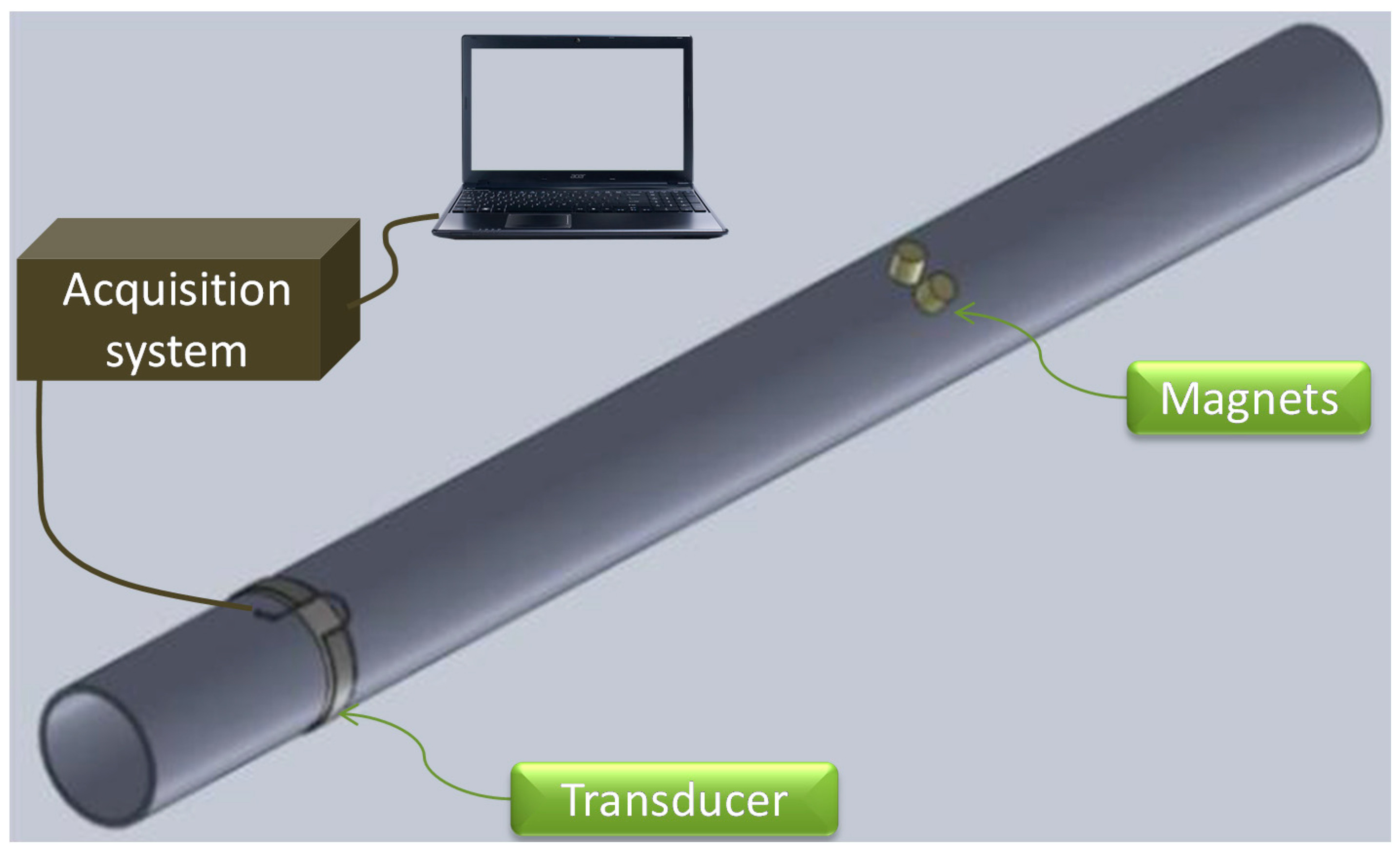
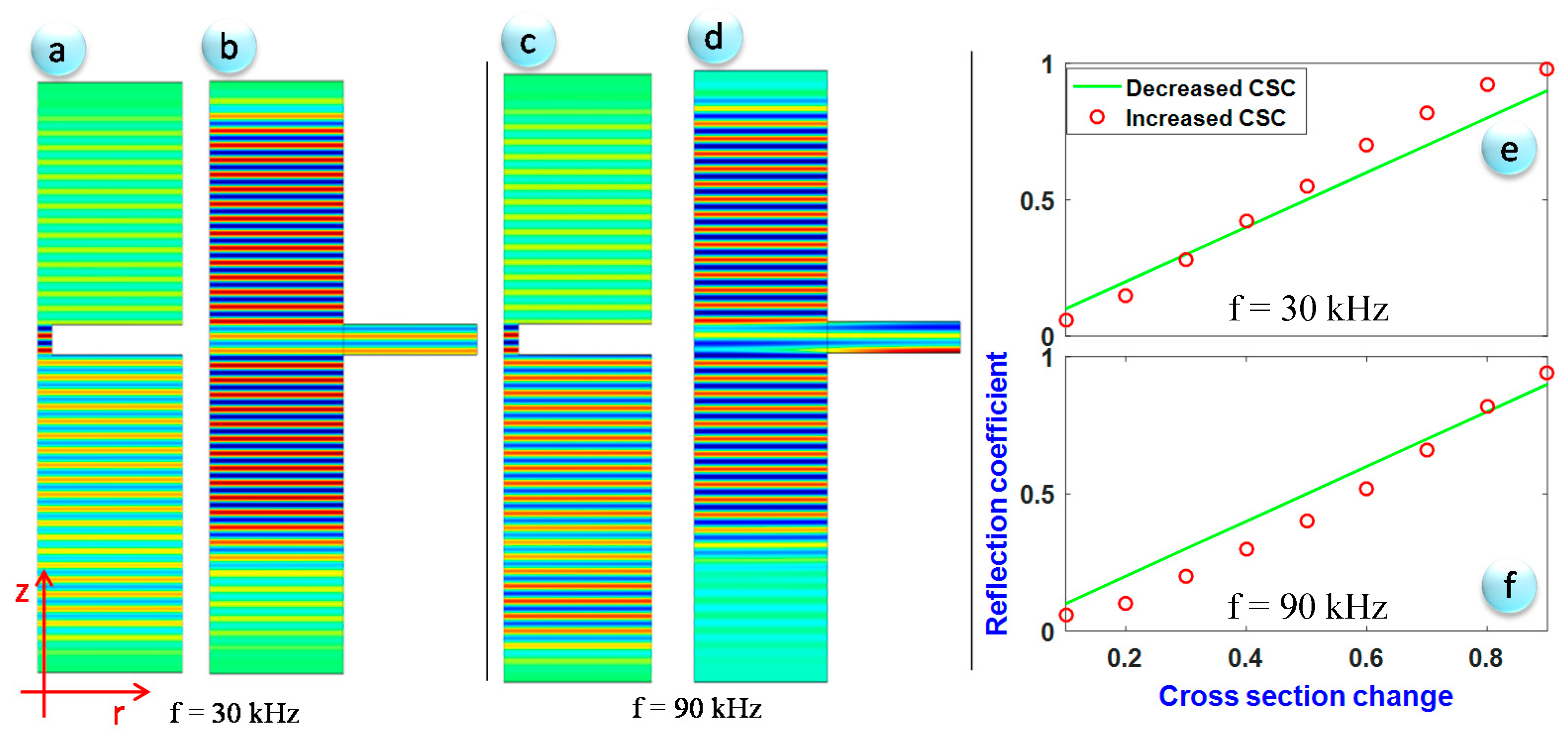
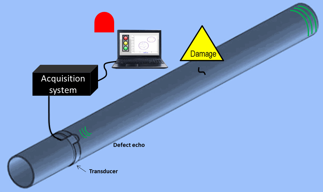
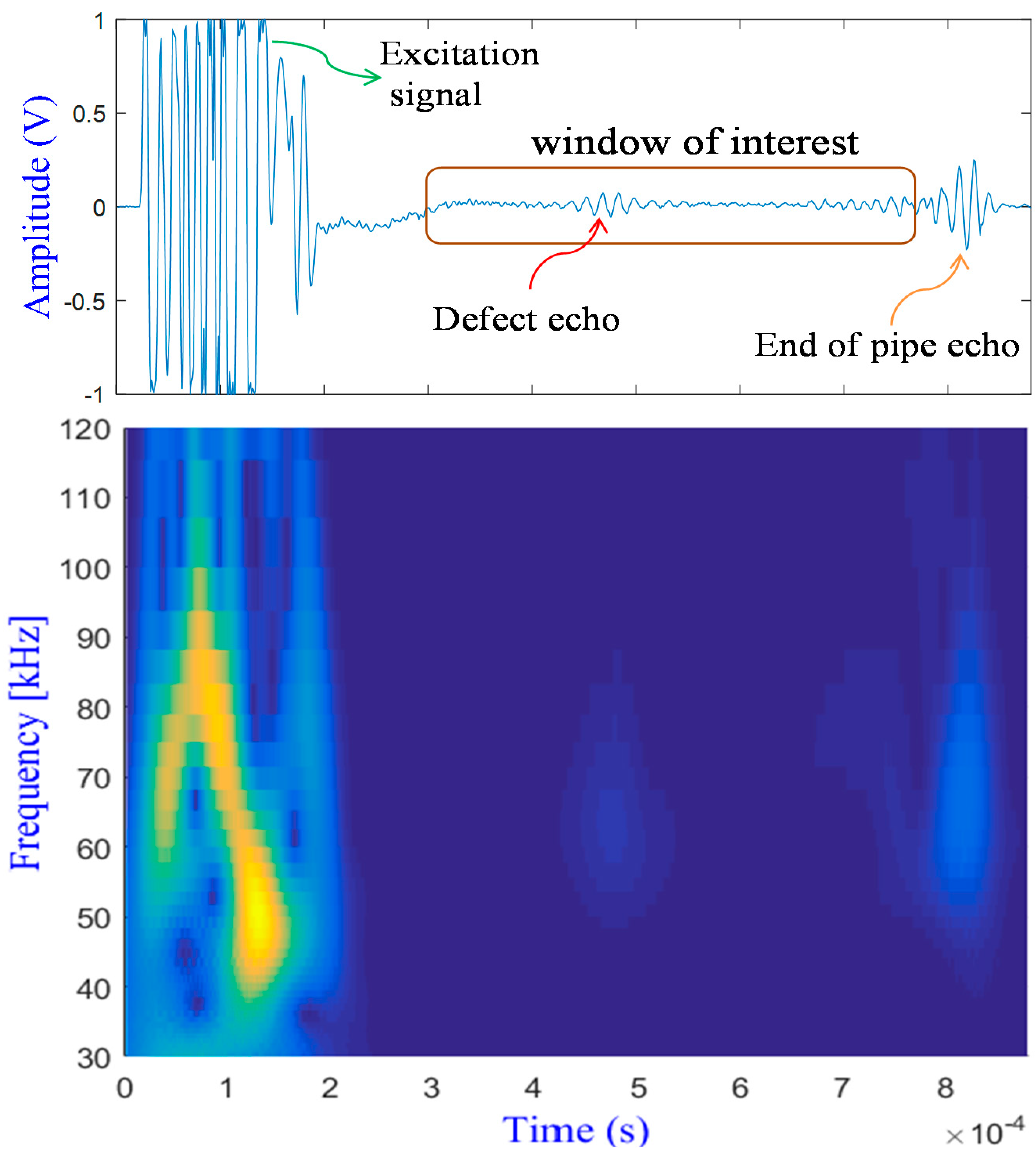
2.1. Guided Waves Based SHM

UGW are stress waves, which propagate through a medium and are guided by the structure’s boundaries. There are two configurations for the generation and the reception of UGW: pitch-catch and pulse-echo [12]. In the former, a transducer can either excite or receive the UGW. In the latter, a transducer can be used for both operations (i.e., generation and reception) [13]. In the current paper, only pulse-echo configuration is used.
When exciting ultrasonic transducers, UGW travel in all directions hence ensuring a volumetric coverage, and they interact with the structure’s discontinuities (this could include damage, welds, structure ends, etc.). At each interaction, the incident wave is decomposed into two parts: reflected wave and transmitted wave. By analyzing the received signal and comparing it with the baseline one, information about the presence of damage can be revealed. However, the task of comparison is not easy to achieve because of the problem of guided wave complexity. In general, UGW involves some propagation phenomena characterized by dispersion, multi-path, and multi-mode components [14]. Therefore, even if the excitation signal is a single echo (typically a toneburst with a few numbers of cycles) and the structure is undamaged, the received signal is very difficult to interpret. Thus, to avoid the interpretation of the signals, the idea is to extract features from the received signals that are sensitive to damage and compare them with those calculated from the reference signals.
The selection of damage-sensitive features is generally based on multiple tests, in order to determine which of these features indicate accurately the presence of damage and are robust to the influence of the structure conditions and environments. The features can be extracted from the time domain (RMS, variance, peak to peak amplitude, maximum amplitude, etc.), frequency domain through Fourier transform, and time-frequency domain using wavelet transform or short Fourier transform. After that, the selected features will be the input of a pattern recognition method that detects defects and estimates (if possible) their size, type, and degree of severity.

2.2. Damage Detection Approach

The following flowchart shown in Figure 1 summarizes all the steps that have been followed to detect the defects.
Based on the work of Hosseini et al. [15], five features can be extracted from the measured signals in the time domain which are: root mean square (RMS), variance, energy, kurtosis, and skewness. In this study, another feature is added, which is the mean. These features are given mathematically as the following:
Mean   ( x ) = 1 N i = 1 N x i
RMS   ( x ) = 1 N   i = 1 N x i 2
Variance   ( x ) = 1 N i = 1 N ( x i Mean   ( x ) ) 2
Energy   ( x ) = i = 1 N x i 2
Kurtosis   ( x ) = 1 N i = 1 N ( x i Mean   ( x ) ) 4 ( 1 N i = 1 N ( x i Mean   ( x ) ) 2 ) 2
Skewness ( x ) =   1 N i = 1 N ( x i Mean   ( x ) ) 3 ( 1 N i = 1 N ( x i Mean   ( x ) ) 2 ) 3
where x is the measured signal and N is the number of the samples x i .

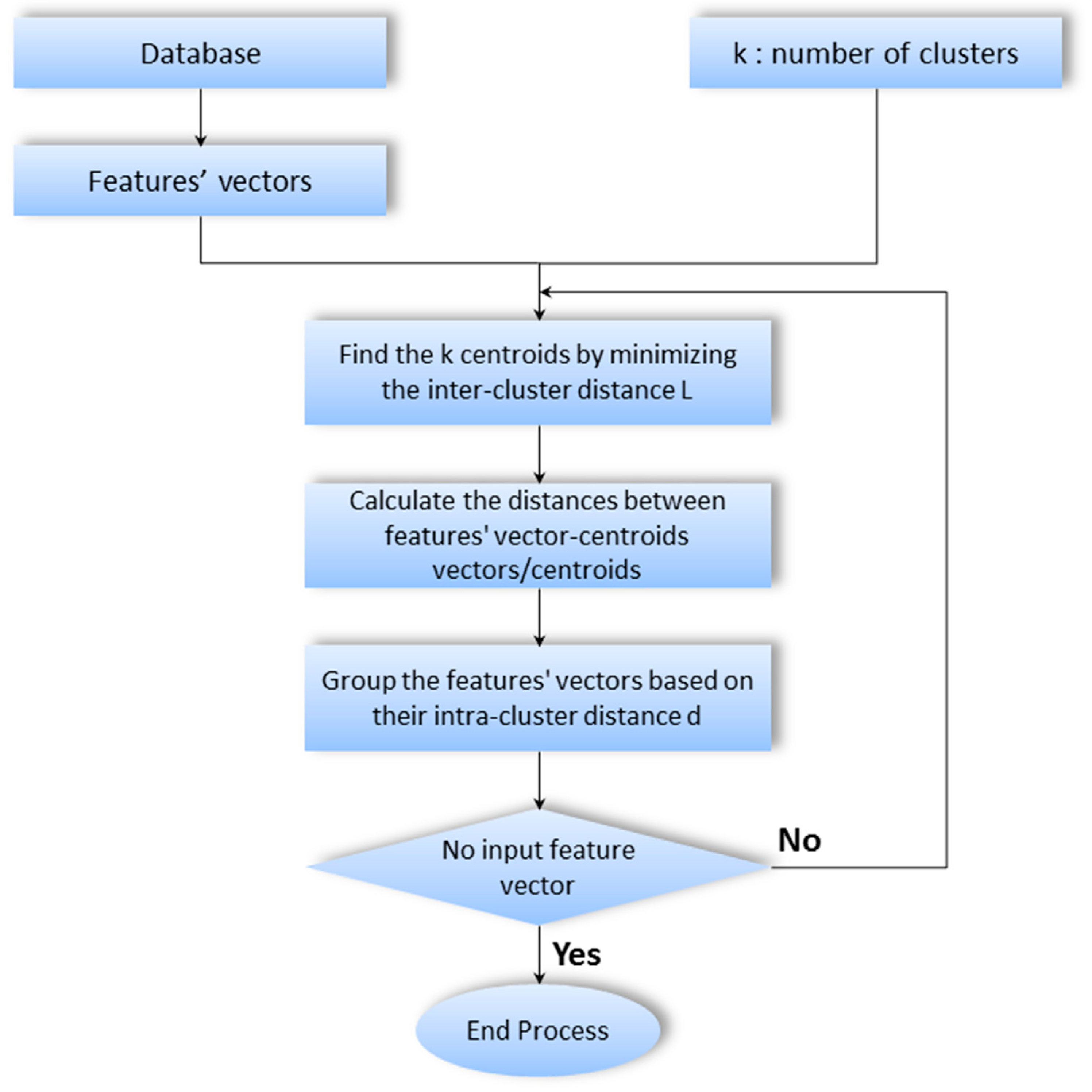
3. K-Means Based Method

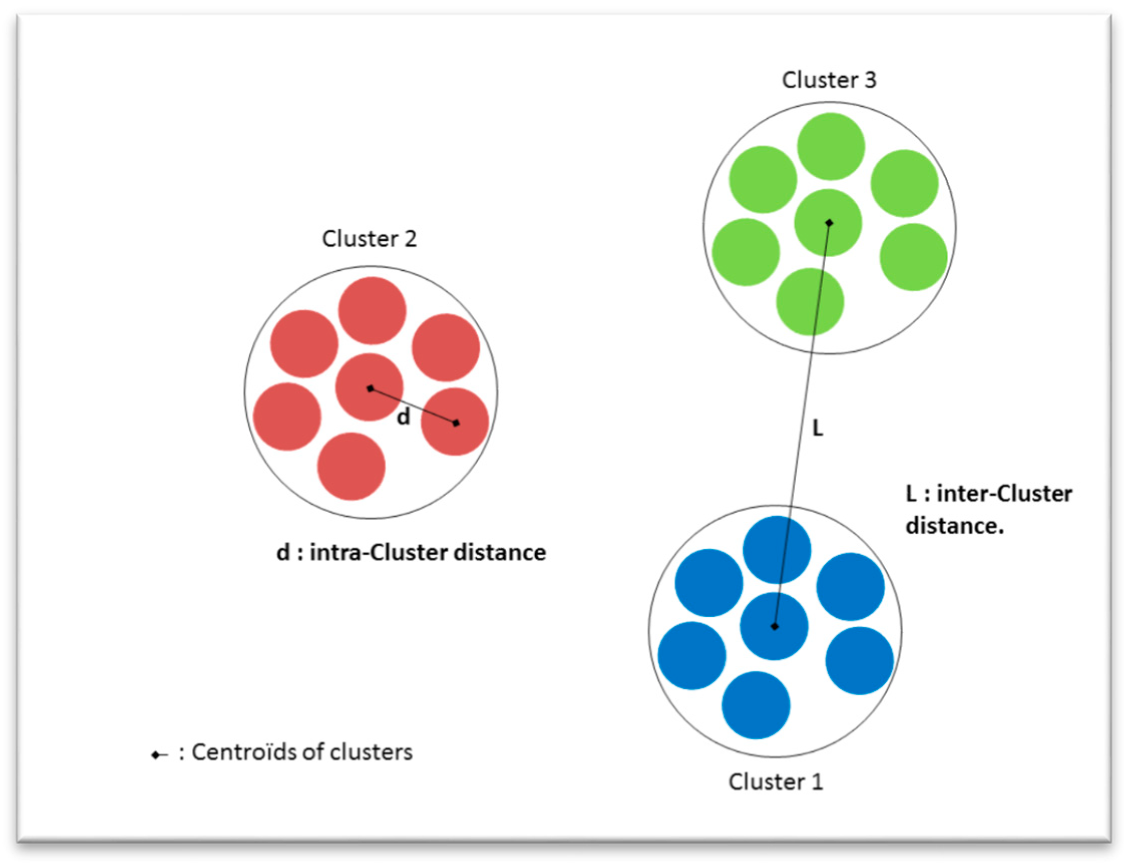
3.1. Classical K-Means Clustering

K-means is an unsupervised learning algorithm used to display similar data in clusters according to a specific metric. The data are represented by a vector of features. The metric is then measured by calculating the distance between the vectors. The purpose of clustering is to regroup data in k separated clusters based on their feature vector distances. Indeed, there are different ways to measure the distance but the choice of an optimal one is generally based on the data set and the targeted output. The performance of this algorithm can be estimated by the matching matrix, which indicates the percentage of correctly classified data and the false alarm rate as in the case of supervised learning [16].
The k-means algorithm can be defined as follows: given a vector of data (features data) and a number of desired clusters k, the idea is to find k centers that minimize the distance of each vector to its nearest center. Note that the k-means is considered as a computationally difficult problem (NP hard). However, many heuristic algorithms were proposed that converge quickly to an optimum. Lloyd’s algorithm [17] is one of them and can be described with the following steps:
  • Randomly choose k points (centers) from the input data set;
  • Extract feature vectors from data;
  • Assign each feature vector to the closet center;
  • Compute the new centers of the formed clusters.
Steps 3 and 4 are repeated until the centers and the clusters of each factor vector do not change. Following this approach, Lloyd’s algorithm will always converge to a solution, but choosing different initial centers will probably lead to different clustering boundaries. That is why the algorithm must be repeated many times to make sure that the clusters are the same—or if there is any difference, choose the one that exhibits good homogeneity and good separation between the clusters.
At each iteration, the k-means algorithm minimizes the intra-cluster distance (i.e., the distance between an element and the centroid of the same cluster). An illustration is shown in Figure 2. Repeating the k-means clustering several times with different initial centers leads to maximizing of the inter-cluster distance (i.e., the distance between the k centroids of clusters). Different metrics are used to calculate the minimized and maximized distances, such as Euclidian distance, Mahalanobis distance [18], Manhattan distance [19], etc. An illustration of the Lloyd’s algorithm is provided in Figure 3.

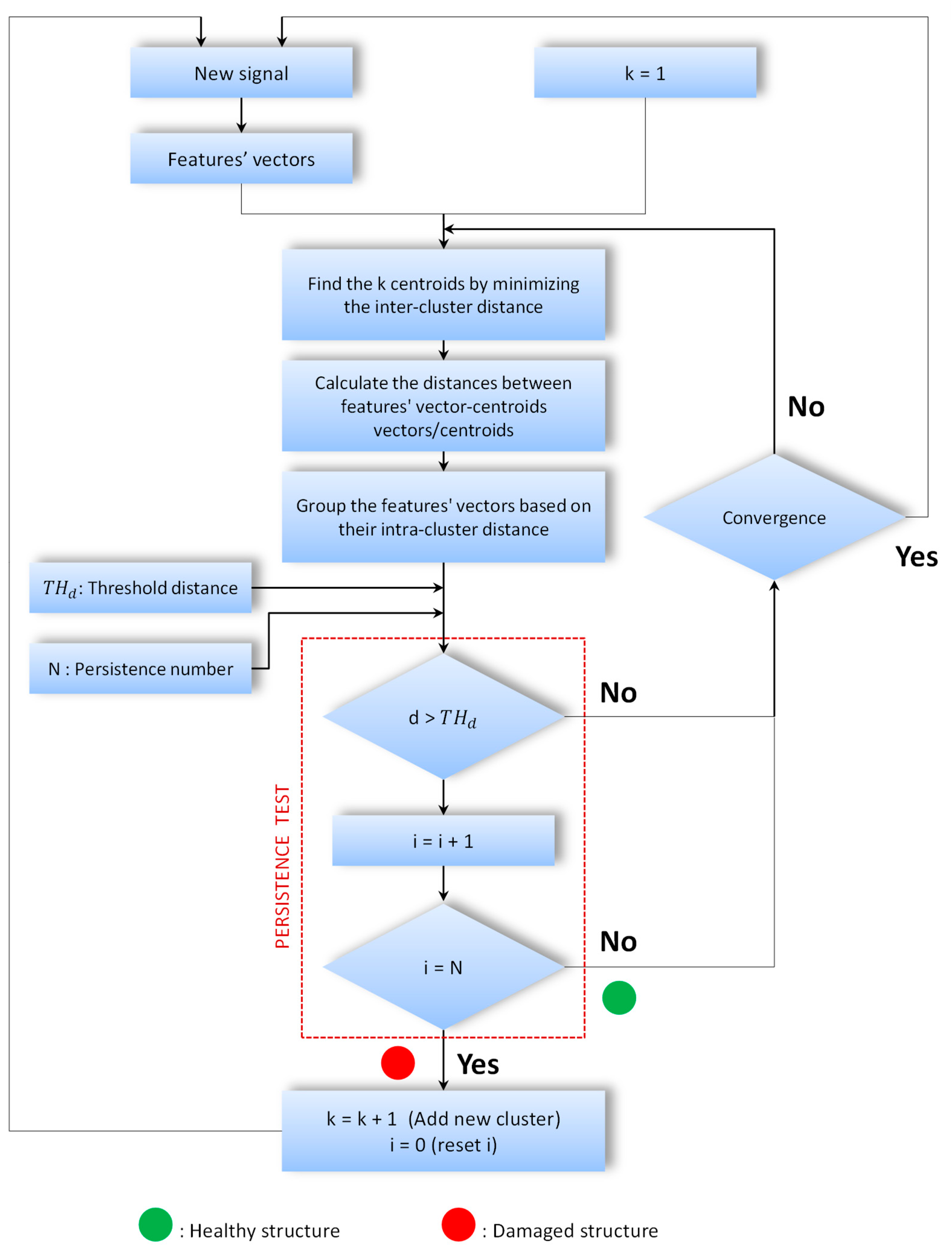
3.2. Proposed Online Damage Detection Method

Actually, the k-means clustering method is used after collecting all the signals corresponding to the different pipeline states (damaged and healthy). In a real industrial application, the detection of a defect has to be accomplished once the damage is initiated. In other words, the damage detection method should be able to detect the early stage defect before it can reach a critical size. In this case, the previous algorithm has to be modified in order to allow the k-means to track the defect. Figure 4 presents the new flowchart of this algorithm.
  • TH d : threshold of limit value of the distance that can be considered in the same cluster;
  • i: counter of signal distances that exceed TH d ;
  • k: number of clusters;
  • N: persistence number to reach a new cluster;
  • d: the Euclidian distance between the new signal feature vector and the centroid of its cluster.
The proposed method starts the clustering when the first signal is acquired. Initially, the number of clusters is k = 1. The classical k-means steps are followed to extract feature vectors, find the initial centroids, calculate the distances between feature vectors and the centroids, and then cluster the feature vectors. A persistence test is added to this process. Actually, if the distance between the new signal and the centroid is higher than a fixed threshold distance TH d , a counter i is incremented. When the value of i is equal to the fixed persistence number N, a new cluster is created by incrementing k. The clustering process restarts with the new number of clusters, the k-means algorithm converges when the feature vectors do not update their cluster label.

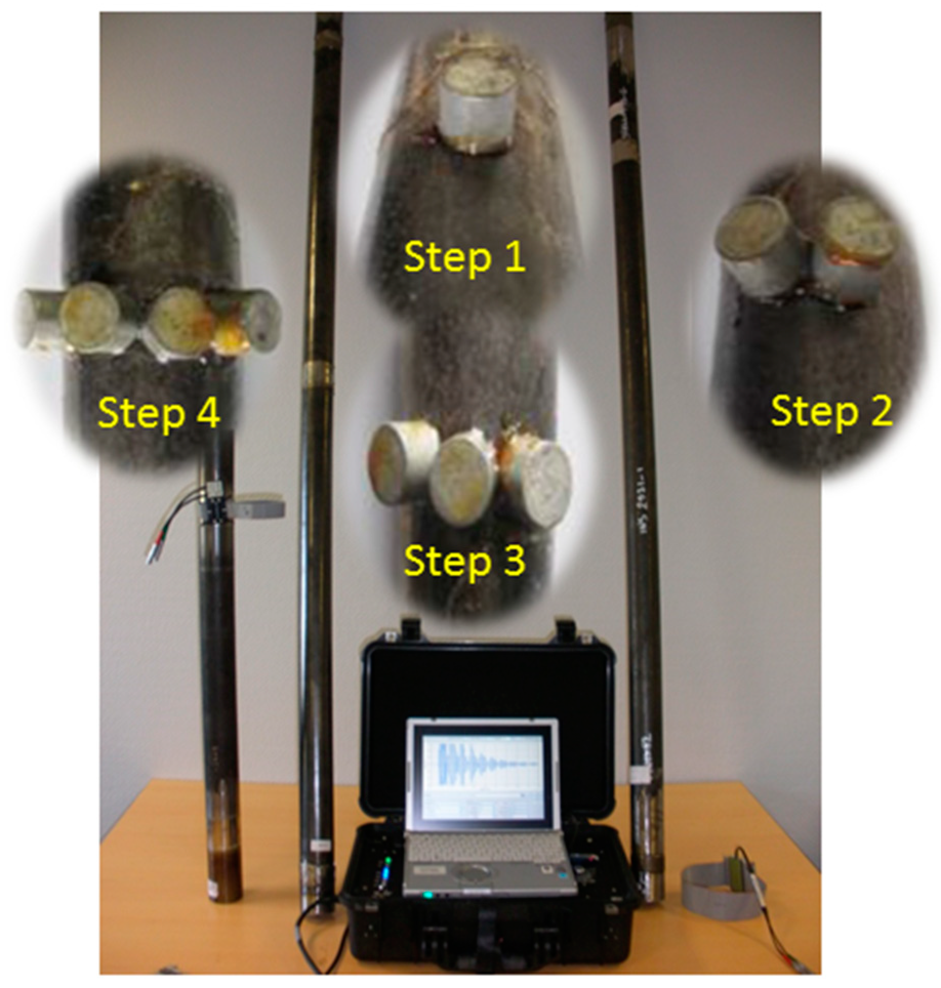
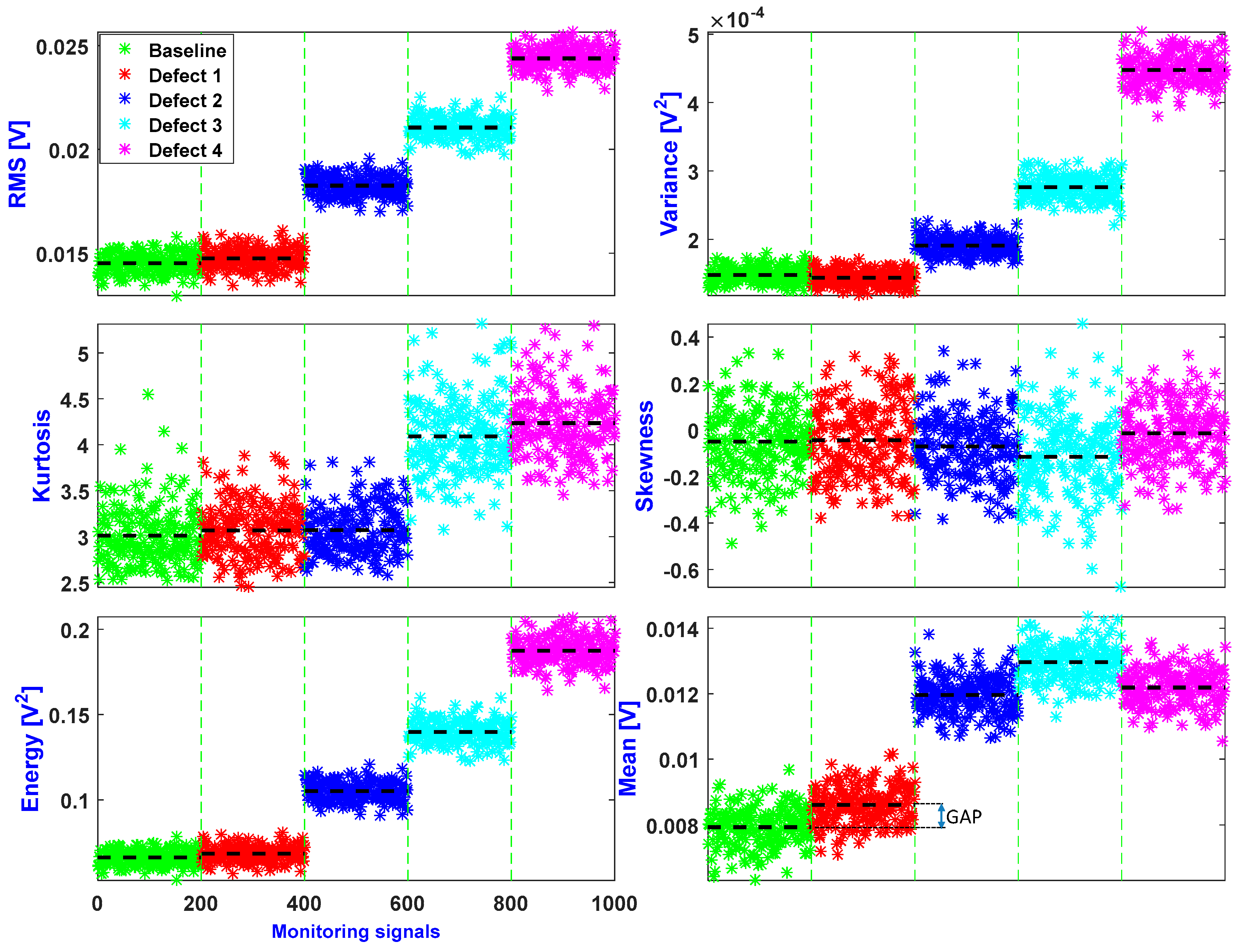
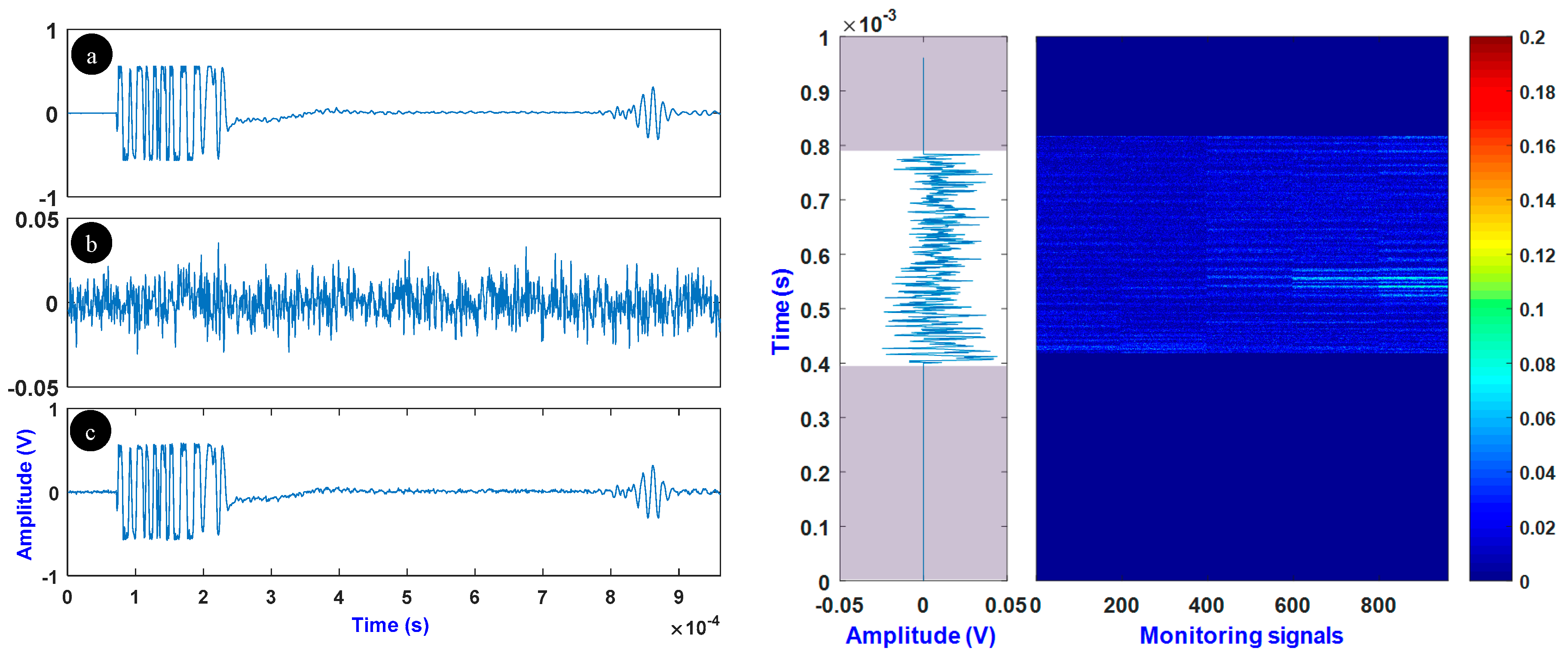
4. Experiments and Database Building

The experiments were conducted on a 2 m steel tube placed in laboratory conditions. Data acquisition was performed using a commercial system designed initially for in situ nondestructive testing of tubular structures using UGW. This system was connected to a magnetostrictive sensor [20], which was mounted on the tube. Figure 5 shows this system.
To help understand this experimental setup, a schematic diagram is shown in Figure 6. In this study, damage was simulated by attaching magnets to the structure, as shown in Figure 5. This choice was made to keep the tube safe (i.e., healthy) in order to use it in other experiments, and to repeat any previous task if the corresponding result was not satisfying. Such a method for simulating damage was applied in different research works [21,22]. Actually, defect occurrence in a structure can be geometric (i.e., local change of the shape of the structure) or material (i.e., local change of the stiffness of the material). The magnet is not used in order to induce a change in the stiffness of the steel, but to locally modify its geometry. Hence, it will not simulate a corrosion-like defect because it is not a loss of material, but another kind of defect with regard to UGW, such as a weld, pipe support, etc. By doing so, UGW will interact with such a defect. Moreover, thanks to its magnetic force, the magnet can be attached to the structure without any other tool. That is to say, the magnet can be replaced by a small piece of steel.
For illustration, Figure 7 shows the result of a finite element numerical simulation of UGW propagating in two different cases: a structure with loss of material (i.e., decreased cross-section change (CSC)), and the same structure with added material (i.e., increased CSC). The simulation was achieved in the frequency domain with the same parameters, for two central frequencies: 30 and 90 kHz. The results show that in the case of added material, the reflection coefficient of UGW was quasi-similar to the case of loss of material.
Damage growth was performed by increasing circumferentially the number of magnets. Other cases were studied in order to assess the influence of the defect orientation on its detectability. For the sake of brevity, this item is not discussed in this paper and the corresponding results are not shown here. It is worth noting that due to the reversibility of this technique of creation of artificial damage, testing the developed damage detection method on an in-service structure could be possible [23]. Furthermore, the magnets can be simply moved along the structure to test the efficiency of damage localization methods [24].
An example of a received signal with its time-frequency representation is given in Figure 8. This signal was obtained with an excitation frequency of 64 kHz using the pulse-echo configuration. The sampling frequency was set at 1 MHz. The signal contains mainly three echoes: the first one, from left to right, corresponds to the excitation, the second one to the defect, and the third one to the end of the tube.
The excitation echo and the one corresponding to the end of the pipe were excluded from the received signal because damage signatures were trapped between them. Thus, only the window of time signal between these echoes was retained. This window was chosen by retaining the signal between the time interval 0.25–0.784 ms. Note that no precision was required, and that this time interval could have been even shorter. The only requirement was to avoid the echo of the excitation (the first echo in the signal) and the echo reflected by the end of the pipe. The later one can simulate, in the case of in-service pipe, a support, a weld, etc. Since the echo generated by the defect is always very small comparatively to that/those produced by permanent reflectors, such as a support, weld, etc., the echoes corresponding to the said reflectors can mask the presence of the defect. Therefore, it is judicious to extract only the region where we suspect the presence of damage. Furthermore, such representation of the measured signals will also help to minimize computation time of signal features by reducing vector dimensions. The analysis was limited to the time domain, in which various features described in Section 2.2 were extracted. The time-frequency analysis is shown here just to give an idea about the frequency content of each echo. An apparent difference can be remarked in frequency bandwidth by comparing the echo of the defect with that of the end of the tube.
For the purpose of testing the performance of the proposed k-means algorithm, an additive white Gaussian noise was added to the collected signals with a specific level. This variation in the signal-to-noise ratio (SNR) can be caused in practice by a number of factors, including changing electrical power to the ultrasonic transmitter, changing sensor/structure ultrasonic transduction efficiency, etc. Besides, adding the noise helps to increase the statistical population of the data.
The noise signals were generated by the MATLAB randn function. This function was multiplied by a factor that determines the noise level. In the present study, this factor was equal to 0.01. For each acquisition, the randn function was called 200 times and added to the collected signal. Hence, a database of 1000 signals was generated (200 signals for the healthy state and 200 signals for each damage state). It is notable that each time the function randn was called, it generated different values but always with a zero mean and a standard deviation equal to the specified noise level. All the preprocessed signals (i.e., 1000) were gathered in a matrix and plotted in Figure 9 (right).
In order to quantify how the signals were buried in noise, a measure of the SNR was necessary [25]. Its mathematical formula can be expressed as follows:
SNR = ( RMS signal RMS noise )
with
RMS signal = 1   N i = 1 N s i 2   and   RMS noise = 1   N i = 1 N n i 2
where s i   and n i   correspond to signal and noise instantaneous amplitudes, respectively.
Figure 10 (left) shows an example of an original signal, a noise signal, and the corrupted signal (SNR = 19 dB). Note that, when the excitation echo and the end of pipe echo were excluded, the SNR drops to 3 dB. The matrix of data, obtained after removing the excitation and the end of pipe echoes, is shown in Figure 10 (right).

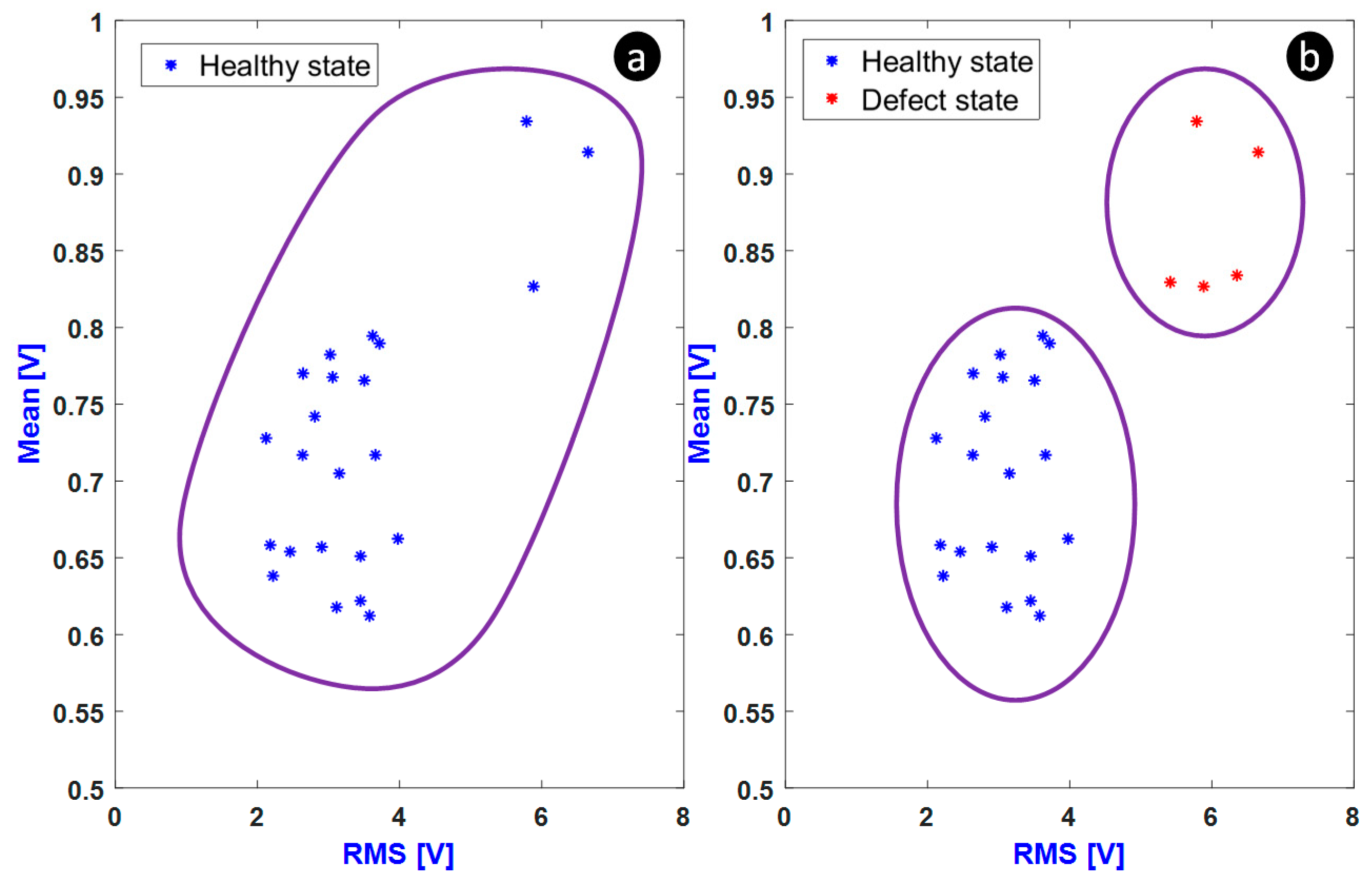
5. Results and Discussion

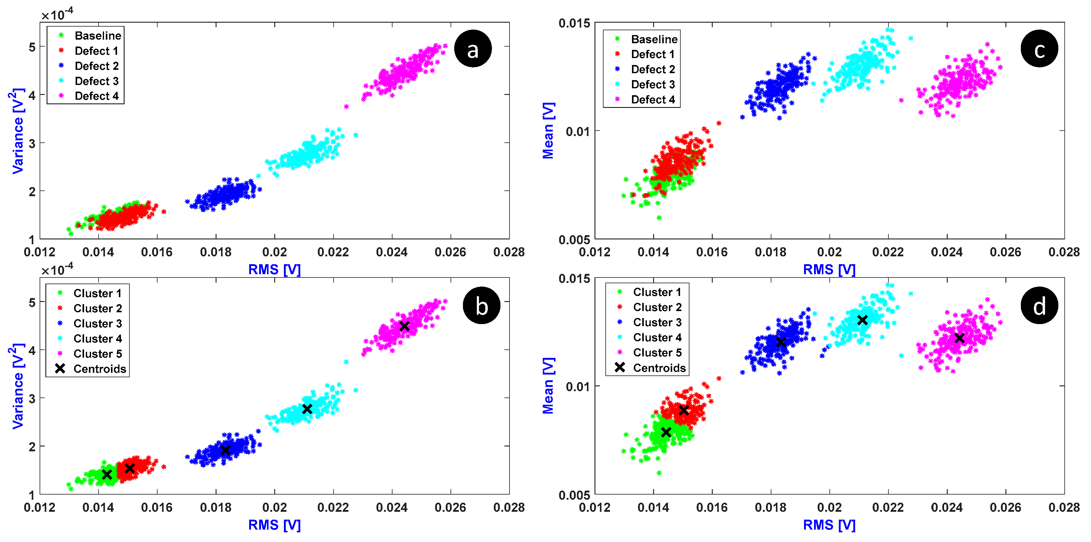
5.1. Classical K-Means

The result of the features provided in Section 2.2 is presented in Figure 11. In order to retain damage-sensitive features and exclude insensitive ones, feature selection was performed. This figure shows that the kurtosis and skewness had poor power of discrimination between all damage states. Consequently, these two features were excluded from the final set of relevant features. Energy and RMS had similar behavior towards the data. Thus, one of them was redundant and was removed (in this study, energy was discarded). Variance and mean had different behaviors and hence they were retained. Finally, the retained features were: RMS, variance, and mean.
To evaluate the discriminatory power of these features, each signal was represented in two-dimensional spaces by two features, namely ( RMS ,   variance ) and ( RMS ,   mean ) . Note that the case ( variance ,   mean ) is not shown here because it was similar to the first case. Consequently, a feature vector is defined as the following:
Feature   vector = ( Feature   1   , Feature   2 )
where ( Feature   1   , Feature   2 ) is either ( RMS ,   variance ) or ( RMS ,   mean ) .
The feature vectors were used as input for the k-means algorithm. The distance used in the k-means algorithm was the Euclidian distance. In order to validate this algorithm, the k-means clustering result was repeated 50 times with different random locations of the k centroids. The clustering process was applied with the defined feature vectors using a number of cluster k = 5, which corresponds to {‘Healthy’, ‘Defect 1’, ‘Defect 2’, ‘Defect 3’, ‘Defect 4’} as previously explained. The results are shown in Figure 12.
The k-means algorithm converged with less than 20 iterations, but the two first clusters found by the k-means did not exactly correspond to the real clusters in both cases: (RMS, variance) and (RMS, mean). The clusters with a high inter-cluster distance were perfectly determined by the k-means (i.e., Cluster 3, Cluster 4, and Cluster 5). In the case of overlapped data (Cluster 1 and Cluster 2), the k-means algorithm could not separate the signals according to their original clusters.
In order to evaluate the accuracy of the clustering process with the k-means for both feature vectors, we used the matching matrix shown in Table 1 and Table 2. This matrix allows the visualizing of the accuracy of the k-means results by comparing the actual cluster of each signal from the database to the predicted cluster given by the k-means. The rows of this matrix are the actual classes of the signals and the columns are the predicted classes of the signals. For instance, the first value of this matrix is the percentage of the signals that were predicted as baseline and they were actually from a healthy pipe. The second value at right gives the percentage of the signals that were predicted as ‘Defect 1’ signals, but in reality, they were from a healthy pipe and so on. Note here that these values were computed by manually assigning the classes of the found clusters by the k-means algorithm unlike supervised learning methods where the labels of the signals are a priori known.
The results of Table 1 show that the percentage of good classification of the two overlapped clusters (i.e., ‘Healthy’ and ‘Defect 1’) drops to 52.5% for the case of (RMS, variance). This can be explained by the fact that the RMS and the variance cannot separate the healthy state from the one with the smallest defect. As it can be remarked, when the defect reaches the level of Defect 2, its percentage of good classification jumps to 99%. When the size of defect increases, the values of the RMS and variance increase as well. At this stage, it can be concluded that the RMS and the variance of the signals allow tracking of the growth of the defect.
The results of Table 2 show a higher percentage of good classification for the two first clusters. In other words, the feature vector (RMS, mean) better discriminates the Defect 1 data from the healthy state data. Comparatively to the (RMS, variance) feature vector, the (RMS, mean) is more relevant since it allowed the obtaining of higher damage sensitivity.
As mentioned previously, the k-means algorithm requires the number of clusters “k” as an input. However, it is always difficult to expect the optimal number of clusters, without calling some specific criteria. In the literature, different criteria can be found. For instance, the Calinski–Harabasz [26] clustering criterion is chosen when the Euclidean distance is used as metric to calculate distance between feature vectors (which is the case in this work). This criterion is based on the sums of squared Euclidean distances between the feature vectors and the centroids of the predicted clusters. The optimal number of clusters is then obtained by identifying the minimum value of this clustering criterion. Another clustering criterion is the Silhouette index [27,28]. This criterion is based on the difference between inter-cluster distances calculated as the smallest average distance between a feature vector and all the feature vectors of other clusters (the bigger the value of this distance corresponds to a good separation of clusters) and the intra-cluster distances are defined as the average distance between a feature vector and all the other vectors in the same cluster (the smallest value of intra-cluster distance corresponds to a better similarity between the feature vectors of the cluster). This value is then normalized to get the Silhouette index which is included in [ 1 ,   1 ] range. The Silhouette index evaluates the cohesiveness of a cluster. The optimal number of clusters is obtained by maximizing the value of this index. The Davies–Bouldin criterion [29] uses also the intra-cluster and the inter-cluster distances. This criterion processes each cluster individually and evaluates its similarity to the nearest cluster. Then, it calculates the mean value of these similarities, and in this case, the optimal number of clusters is obtained by minimizing this criterion in order to have low similarity between the clusters. Finally, the gap statistic criterion [30] is based on the logarithmical mean of the pairwise distances of all the feature vectors. It determines the optimal number of clusters by applying the “elbow method” [31].
The above mentioned criteria for evaluating the optimal number of clusters k were applied for the cases of the two feature vectors. The result is shown in Figure 13. In the first case as shown in Figure 13a, which concerns the feature vector (RMS, variance), all the criteria agree that the optimal number of clusters is kOPT = 4. In the second case as shown in Figure 13b, which concerns the feature vector (RMS, mean), only the gap criterion indicates that the optimal number of clusters is five, which is the real number of data groups. This confirms that the feature vector (RMS, mean) is the most relevant for damage detection and will be retained in the following development.
It is worth noting that the sensitivity of the proposed method for damage detection at different locations of damage depends on the SNR. In general, the SNR decreases as the distance between emitter/receiver and the defect increases. This is due to the attenuation of UGW, which can be mainly caused in pipes, by leakage in the inner medium (transported fluid, for example), and outer medium (coating, for example). However, in the current study, the tube was empty and bare. Consequently, the attenuation was quasi-absent. In addition, the statistical features were extracted from the whole region of interest in the acquired signal. Therefore, the position of the defect echo, in the signal, should not have an influence on the result.

5.2. Novel Proposed Method

The proposed method in Figure 4 was implemented as an online clustering process. The 200 signals corresponding to Defect 1 were not used since they were overlapping with the 200 healthy signal states. To illustrate the working principle of the method, let us consider the example of N = 5 and TH d = 2. The result of Figure 14a shows that the number of signals reaching the fixed TH d was i = 3 while the persistence number N was not reached. Hence, the number of clusters is still k = 1. When the persistence number was reached, the number of clusters was incremented (k = 2) as shown in Figure 14b. As a result, the new cluster represented the presence of a defect.
Different values of the persistence number were tested and two of them were selected: N = 3 and N = 10.
In order to determine the optimal threshold distance value, it was changed from TH d = 4 × 10⁻³ to TH d = 8 × 10⁻³ with a step of 1 × 10⁻³. This range was graphically determined from the previous results shown in Figure 12. The persistence number was fixed at N = 3. The result in Figure 15d shows that a high value of TH d = 8 × 10 3 kept all the signals in the same cluster and hence the number of clusters remained at k = 1. Therefore, this value of TH d did not allow the detection of the damaged state clusters. When TH d = 6 × 10 3 , as shown in Figure 15c, the resulting clustering process was close to the real cluster of signals.
In the case when TH d = 5 × 10 3 , as shown in Figure 15b, the clustering process generated 13 clusters. This was an overestimation of the real number of clusters, which was equal to four. Decreasing the threshold distance value to TH d = 4 × 10 3 , as shown in Figure 15a, led to a larger number of clusters: k = 27. This reduced the usefulness of clustering since the signals were not well regrouped.
The second clustering process was launched with a persistence number N = 10. This forced the algorithm to verify the pertinence of the creation of a new cluster. Results are shown in Figure 16. By comparison with the result when N = 3, it can be clearly noticed that the persistence number affected the cluster numbers. In the case when the threshold distance TH d = 6.33 × 10 3 (Figure 16c), the number of clusters was very close to the real number of clusters.

6. Conclusions

In this paper, a SHM method for damage detection in pipelines was proposed. It relies on the use of the k-means method for clustering the data collected during monitoring by means of an ultrasonic guided waves technique. Feature extraction and selection were performed on the created database in order to determine features that were more sensitive to the presence of damage. Results have shown that the use of features (RMS, mean) with the gap statistic criterion used to evaluate the optimal number of clusters help to automatically detect damage and provide better damage sensitivity.
In order to ensure online monitoring of the pipeline, a modified version of the k-means damage detection method was proposed. It is based on an instant clustering of the presented signals. A defect is detected when a new class of signals is identified. However, this method depends on the threshold distance, which should be fixed in the beginning of the monitoring stage. Also, the persistence parameter, which is used to construct a new cluster, has an influence on the result of damage detection.
As a perspective of this work, the developed online damage detection method will be tested on a pipeline, which serves real environmental variations, such as changes in temperature, flow rate, etc.

Author Contributions

Data curation, A.E.B.; Formal analysis, S.Y.; Investigation, A.E.B. and M.E.M.; Methodology, M.E.M. and S.Y.; Project administration, S.Y.; Resources, F.D.; Software, A.E.B.; Supervision, S.Y.; Validation, A.E.B.; Visualization, M.E.M.; Writing—original draft, A.E.B. and S.Y.; Writing—review & editing, S.Y., M.K. and L.B.; numerical simulations, W.K.

Conflicts of Interest

The authors declare no conflicts of interest.

References

  1. Farrar, C.R.; Worden, K. An introduction to structural health monitoring. Philos. Trans. R. Soc. Lond. A Math. Phys. Eng. Sci. 2017, 365, 303–315. [Google Scholar] [CrossRef]
  2. Lowe, M.J.; Alleyne, D.N.; Cawley, P. Defect detection in pipes using guided waves. Ultrasonics 1998, 36, 147–154. [Google Scholar] [CrossRef]
  3. Zhu, W.; Rose, J.L.; Barshinger, J.N.; Agarwala, V.S. Ultrasonic guided wave NDT for hidden corrosion detection. J. Res. Nondestruct. Eval. 1998, 10, 205–225. [Google Scholar] [CrossRef]
  4. Alleyne, D.N.; Pavlakovic, B.; Lowe, M.J.S.; Cawley, P. The use of guided waves for rapid screening of chemical plant pipework. J. Korean Soc. NDT 2002, 22, 589–598. [Google Scholar]
  5. Rose, J.L.; Avioli, M.J.; Mudge, P.; Sanderson, R. Guided wave inspection potential of defects in rail. Ndt E Int. 2004, 37, 153–161. [Google Scholar] [CrossRef]
  6. Rose, J.L.; Soley, L.E. Ultrasonic guided waves for anomaly detection in aircraft components. Mater. Eval. 2000, 58, 1080–1086. [Google Scholar]
  7. Castaings, M.; Hosten, B. Ultrasonic guided waves for health monitoring of high-pressure composite tanks. Ndt E Int. 2008, 41, 648–655. [Google Scholar] [CrossRef]
  8. Black, S. Structural Health Monitoring: Composites Get Smart, Composites World. September 2008. Available online: https://www.compositesworld.com/articles/structural-health-monitoring-composites-get-smart (accessed on 30 December 2018).
  9. Croxford, A.J.; Moll, J.; Wilcox, P.D.; Michaels, J.E. Efficient temperature compensation strategies for guided wave structural health monitoring. Ultrasonics 2010, 50, 517–528. [Google Scholar] [CrossRef]
  10. Rizzo, P.; Sorrivi, E.; di Scalea, F.L.; Viola, E. Wavelet-based outlier analysis for guided wave structural monitoring: Application to multi-wire strands. J. Sound Vibr. 2007, 307, 52–68. [Google Scholar] [CrossRef]
  11. Eybpoosh, M.; Berges, M.; Noh, H.Y. An energy-based sparse representation of ultrasonic guided-waves for online damage detection of pipelines under varying environmental and operational conditions. Mech. Syst. Signal Process. 2017, 82, 260–278. [Google Scholar] [CrossRef]
  12. Yaacoubi, S.; Chehami, L.; Aouini, M.; Declercq, N.F. Ultrasonic guided waves for reinforced plastics safety. Reinf. Plastics. 2017, 61, 87–91. [Google Scholar] [CrossRef]
  13. Cawley, P.; Lowe, M.J.S.; Alleyne, D.N.; Pavlakovic, B.; Wilcox, P. Practical long range guided wave inspection-applications to pipes and rail. Mater. Eval. 2003, 61, 66–74. [Google Scholar]
  14. Eybpoosh, M.; Berges, M.; Noh, H.Y. Sparse representation of ultrasonic guided-waves for robust damage detection in pipelines under varying environmental and operational conditions. Struct. Control Heal. Monit. 2016, 23, 369–391. [Google Scholar] [CrossRef]
  15. Hossein Abadi, H.Z.; Amir fattahi, R.; Nazari, B.; Mirdamadi, H.R.; Atashipour, S.A. GUW-based structural damage detection using WPT statistical features and multiclass SVM. Appl. Acoust. 2014, 86, 59–70. [Google Scholar] [CrossRef]
  16. Sahu, S.K.; Jena, S.K. A study of K-Means and C-Means clustering algorithms for intrusion detection product development. Int. J. Innov. Manag. Technol. 2014, 5, 207. [Google Scholar] [CrossRef]
  17. Lloyd, S. Least squares quantization in PCM. IEEE Trans. Inf. Theory 1982, 28, 129–137. [Google Scholar] [CrossRef]
  18. Loohach, R.; Garg, K. Effect of distance functions on simple k-means clustering algorithm. Int. J. Comput. Appl. 2012, 49, 7–9. [Google Scholar] [CrossRef]
  19. Singh, A.; Yadav, A.; Rana, A. K-means with three different distance metrics. Int. J. Comput. Appl. 2013, 67. [Google Scholar] [CrossRef]
  20. Kim, Y.G.; Moon, H.S.; Park, K.J.; Lee, J.K. Generating and detecting torsional guided waves using magnetostrictive sensors of crossed coils. Ndt E Int. 2011, 44, 145–151. [Google Scholar] [CrossRef]
  21. Salmanpour, M.S.; Sharif Khodaei, Z.; Aliabadi, M.H. Guided wave temperature correction methods in structural health monitoring. J. Intell. Mater. Syst. Struct. 2017, 28, 604–618. [Google Scholar] [CrossRef]
  22. Alguri, K.S.; Melville, J.; Harley, J.B. Baseline-free guided wave damage detection with surrogate data and dictionary learning. J. Acoust. Soc. Am. 2018, 143, 3807–3818. [Google Scholar] [CrossRef] [PubMed]
  23. Liu, C.; Harley, J.B.; Bergés, M.; Greve, D.W.; Oppenheim, I.J. Robust ultrasonic damage detection under complex environmental conditions using singular value decomposition. Ultrasonics 2015, 58, 75–86. [Google Scholar] [CrossRef] [PubMed]
  24. Ebrahimkhanlou, A.; Dubuc, B.; Salamone, S. Damage localization in metallic plate structures using edge-reflected lamb waves. Smart Mater. Struct. 2016, 25, 085035. [Google Scholar] [CrossRef]
  25. Rostami, J.; Tse, P.W.; Fang, Z. Sparse and Dispersion-Based Matching Pursuit for Minimizing the Dispersion Effect Occurring When Using Guided Wave for Pipe Inspection. Materials 2017, 10, 622. [Google Scholar] [CrossRef] [PubMed]
  26. Caliński, T.; Harabasz, J. A dendrite method for cluster analysis. Commun. Stat. 1974, 3, 1–27. [Google Scholar]
  27. Rousseeuw, P.J. Silhouettes: A Graphical Aid to the Interpretation and Validation of Cluster Analysis. Comput. Appl. Math. 1987, 20, 53–65. [Google Scholar] [CrossRef]
  28. Kaufman, L.; Rousseeuw, P.J. Finding Groups in Data: An Introduction to Cluster Analysis; John Wiley & Sons: Hoboken, NJ, USA, 1990. [Google Scholar]
  29. Davies, D.L.; Bouldin, D.W. A Cluster Separation Measure. IEEE Trans. Pattern Anal. Mach. Intell. 1979, 2, 224–227. [Google Scholar] [CrossRef]
  30. Tibshirani, R.; Walther, G.; Hastie, T. Estimating the number of clusters in a data set via the gap statistic. J. R. Stat. Soc. B 2001, 63, 411–423. [Google Scholar] [CrossRef]
  31. Bholowalia, P.; Kumar, A. EBK-means: A clustering technique based on elbow method and k-means in WSN. Int. J. Comput. Appl. 2014, 105, 9. [Google Scholar]
Figure 1. Flowchart of the proposed damage detection approach.
Inventions 04 00017 g001
Figure 2. Maximized and minimized distances in a k-means clustering process.
Inventions 04 00017 g002
Figure 3. The k-means clustering algorithm.
Inventions 04 00017 g003
Figure 4. Proposed online clustering based on k-means.
Inventions 04 00017 g004
Figure 5. Experimental setup of the guided waves monitoring technique of a tube, and photography showing the adopted method to create a structural defect.
Inventions 04 00017 g005
Figure 6. Schematic diagram of the proposed experimental setup shown in Figure 5.
Inventions 04 00017 g006
Figure 7. Circumferential displacement distribution: for decreased cross-section change (CSC) (a,c), and decreased CSC (b,d), and reflection coefficient versus CSC in both cases (material loss and added material (e,f)). (r, z) are the radial and axial coordinates of the axisymmetric tube.
Inventions 04 00017 g007
Figure 8. Example of a measured signal from a damaged pipe (top) and its time-frequency representation (bottom).
Inventions 04 00017 g008
Figure 9. An example of a collected signal (left), and all the collected data (right).
Inventions 04 00017 g009
Figure 10. (left) Original signal (a), noise (b), and corrupted signal (c), and (right), the collected data after removing the excitation signal and the end of pipe echo and after adding noise.
Inventions 04 00017 g010
Figure 11. Results of the features extracted from the corrupted signals. RMS: root mean square.
Inventions 04 00017 g011
Figure 12. Clustering of collected data using two feature vectors: original clusters for (RMS, variance) (a), k-means clusters for (RMS, variance) (b), original clusters for (RMS, mean) (c), and k-means clusters for (RMS, mean) (d).
Inventions 04 00017 g012
Figure 13. Variation of the criterion of optimal cluster number: (a) (RMS, variance) and (b) (RMS, mean).
Inventions 04 00017 g013
Figure 14. Incrementation of number of clusters (a) k = 1 and (b) k = 2.
Inventions 04 00017 g014
Figure 15. Clustering results with different threshold distance TH d and a fixed persistence number N = 3. (a) TH d = 4 × 10 3 ; (b) TH d = 5 × 10 3 ; (c) TH d = 6 × 10 3 ; (d) TH d = 8 × 10 3 .
Inventions 04 00017 g015
Figure 16. Clustering results with different threshold distance TH d and a fixed persistence number N = 10. (a) TH d = 4 × 10 3 ; (b) TH d = 6 × 10 3 ; (c) TH d = 6.33 × 10 3 ; (d) TH d = 10 × 10 3 .
Inventions 04 00017 g016
Table 1. Matching matrix of the clustering results plotted in Figure 12b.
Predicted Cluster (%)HealthyDefect 1Defect 2Defect 3Defect 4
Real Cluster (%)
Healthy52.547.5000
Defect 147.552.5000
Defect 2009910
Defect 3000.599.50
Defect 40000100
Table 2. Matching matrix of the clustering results plotted in Figure 12d.
Predicted Cluster (%)HealthyDefect 1Defect 2Defect 3Defect 4
Real Cluster (%)
Healthy7129000
Defect 13565000
Defect 2009820
Defect 3001.598.50
Defect 40000100

