Distributed Strain Sensing from Different Optical Fiber Configurations


Abstract
:
1. Introduction
2. Distributed Fiber Optic Sensing
3. Analytical Approach
4. Materials and Fabrication
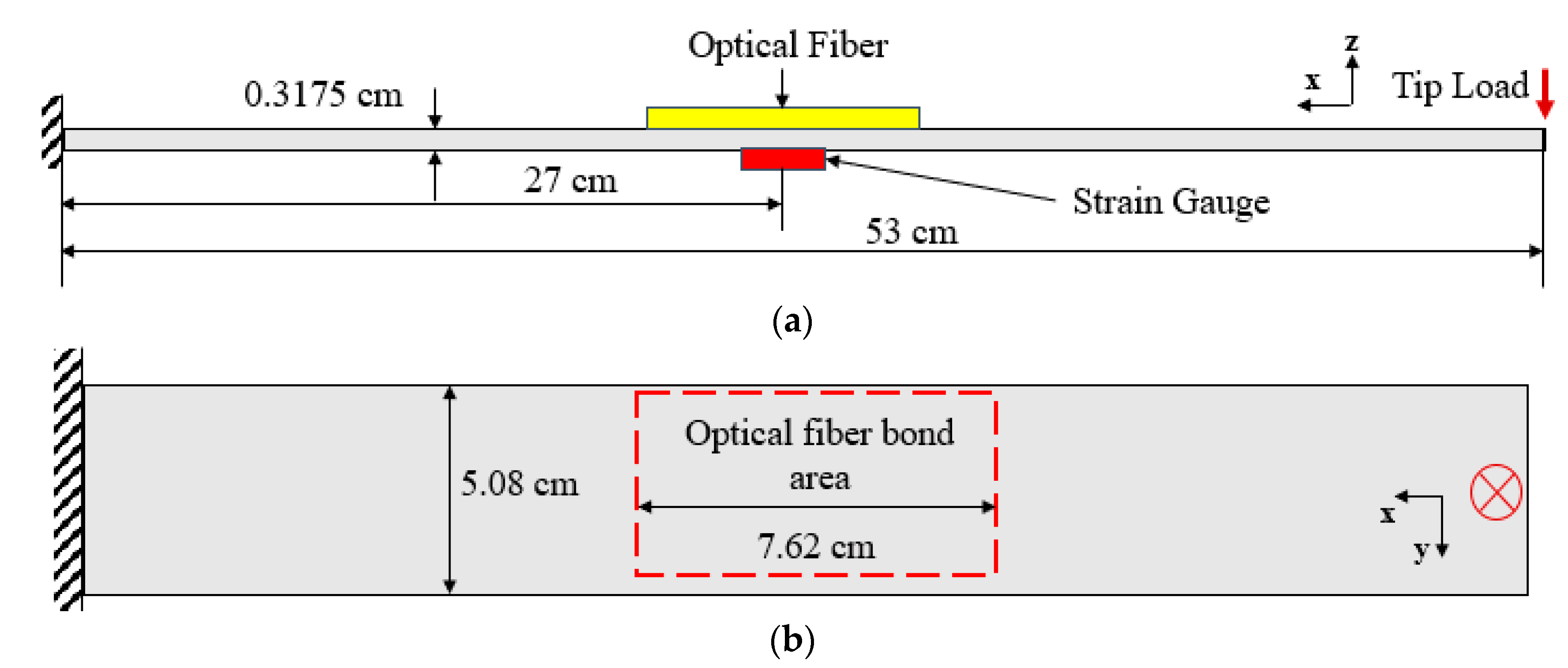
- At the mid-span of each beam (Figure 2a), a 7.62 cm by 5.08 cm area was sanded with 600 grit sand paper and cleaned using 99% isopropanol.
- Light pencil marks were placed on the surface of the aluminum beam away from the bonded area to use as reference points to place the optical fiber.
- Optical fibers were placed onto each aluminum beam and held in each configuration using Kapton tape.
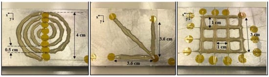
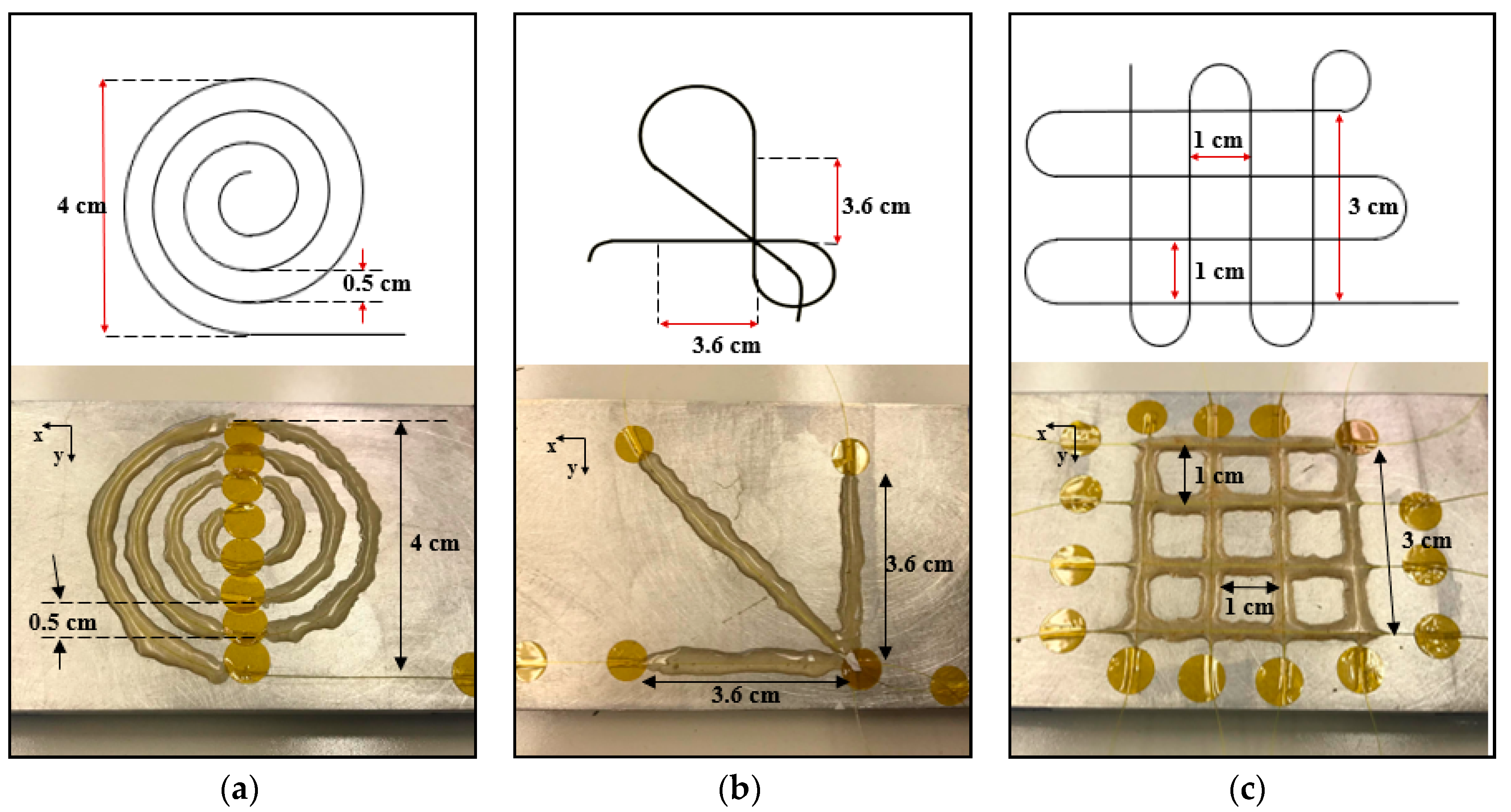
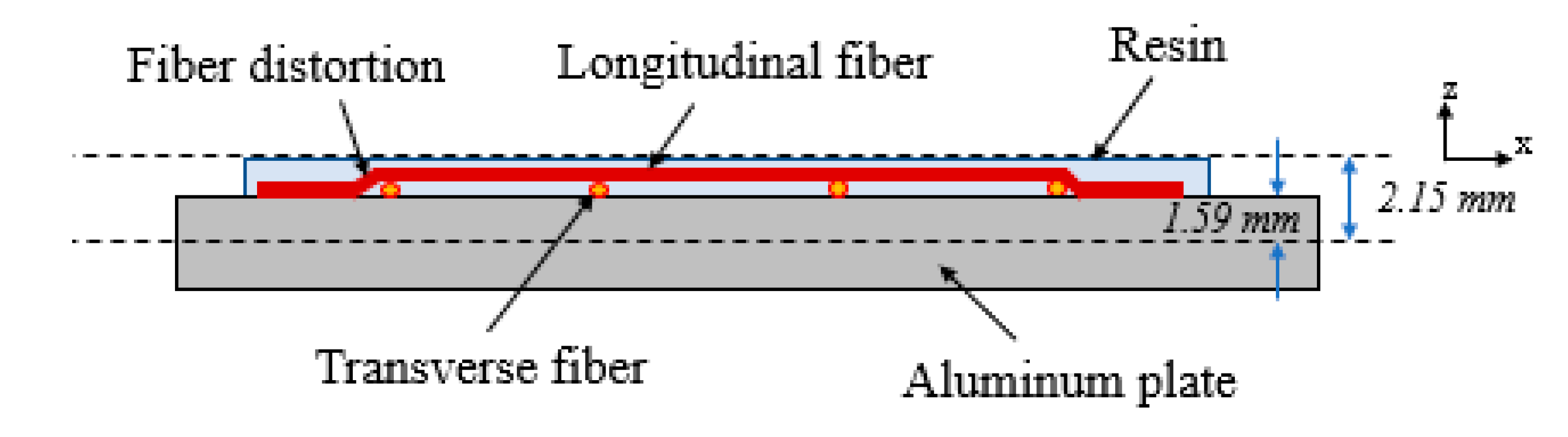
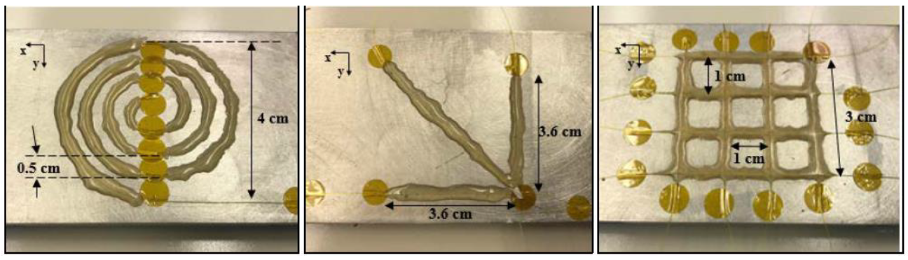
- The optical fiber was adjusted until the desired dimensions were accurately reached (shown in Figure 3). This was performed by gently peeling back the Kapton tape to adjust the optical fiber and add a slight pretension to maintain alignment.
- M-Bond AE-10 resin with GA-2 curing agent was used to adhere the fiber to the surface of the aluminum. This was applied by spreading resin on top of the optical fiber using a thin glass rod. The optical fiber was gently prodded to ensure resin was around the perimeter of the fiber.
- The adhesive was cured at room temperature for approximately two hours.
5. Experimental Procedure
6. Results and Discussion
7. Conclusions
Author Contributions
Funding
Conflicts of Interest
References
- Minakuchi, S.; Takeda, N.; Takeda, S.-I.; Nagao, Y.; Franceschetti, A.; Liu, X. Life cycle monitoring of large-scale CFRP VARTM structure by fiber-optic-based distributed sensing. Compos. Part A Appl. Sci. Manuf. 2011, 42, 669–676. [Google Scholar] [CrossRef]
- Grave, J.H.L.; Haheim, M.L.; Echtermeyer, A.T. Measuring changing strain fields in composites with Distributed Fiber-Optic Sensing using the optical backscatter reflectometer. Compos. Part B Eng. 2015, 24, 138–146. [Google Scholar] [CrossRef]
- Davis, C.; Knowles, M.; Rajic, N.; Swanton, G. Evaluation of a Distributed Fibre Optic Strain Sensing System for Full-Scale Fatigue Testing. Procedia Struct. Integr. 2016, 2, 3784–3791. [Google Scholar] [CrossRef]
- Batte, L.K.; Sullivan, R.W.; Ranatunga, V.; Brown, K. Impact response in polymer composites from embedded optical fibers. J. Compos. Mater. 2018. [Google Scholar] [CrossRef]
- Choi, B.-H.; Kwon, I.-B. Strain pattern detection of composite cylinders using optical fibers after low velocity impacts. Compos. Sci. Technol. 2018, 154, 64–75. [Google Scholar] [CrossRef]
- Drake, D.; Sullivan, R.W.; Spowart, J. Cure Monitoring of CFRP Composites using Embedded Optical Fibers. In Proceedings of the 56th AIAA Aerospace Science Meeting, AIAA Scitech Forum, Kissimmee, FL, USA, 8–12 January 2018. [Google Scholar]
- Meadows, L.; Sullivan, R.W.; Brown, K.; Ranatunga, V.; Vehorn, K.; Olson, S. Distributed optical sensing in composite laminates. J. Strain Anal. Eng. Des. 2017, 52, 410–421. [Google Scholar] [CrossRef]
- Gifford, D.K.; Soller, B.J.; Wolfe, M.S.; Froggatt, M.E. Distributed fiber-optic temperature sensing using Rayleigh backscatter. In Proceedings of the 2005 31st European Conference on Optical Communication, ECOC 2005, Glasgow, UK, 25–29 September 2005; pp. 511–512. [Google Scholar]
- Kreger, S.T.; Gifford, D.K.; Froggatt, M.E.; Soller, B.J.; Wolfe, M.S. High Resolution Distributed Strain or Temperature Measurements in Single- and Multi-Mode Fiber Using Swept-Wavelength Interferometry. In Proceedings of the Optical Fiber Sensors, Cancun, Mexico, 23–27 October 2006. [Google Scholar]
- Soller, B.J.; Wolfe, M.; Froggatt, M.E. Polarization Resolved Measurement of Rayleigh Backscatter in Fiber-Optic Components. In Proceedings of the Optical Fiber Communication Conference and Exposition and The National Fiber Optic Engineers Conference, Anaheim, CA, USA, 6–11 March 2005. [Google Scholar]
- Hibbeler, R.C. Mechanics of Materials, 6th ed.; Pearson Prentice Hall: Upper Saddle River, NJ, USA, 2005. [Google Scholar]
- Antunes, P.; Domingues, F.; Granada, M.; André, P. Mechanical Properties of Optical Fibers. In Selected Topics on Optical Fiber Technology; Yasin, M., Ed.; InTech: London, UK, 2012; ISBN 978-953-51-0091-1. [Google Scholar] [Green Version]
- Abang, A.; Webb, D.J. Influence of mounting on the hysteresis of polymer fiber Bragg grating strain sensors. Opt. Lett. 2013, 38, 1376–1378. [Google Scholar] [CrossRef] [PubMed] [Green Version]
- Alexandar, D.; Marijana, F.; Richard, Y.K.F. Principles of deflection-curvature measurement. Meas. Sci. Technol. 2001, 12, 1983. [Google Scholar]
- Di, H.; Xin, Y.; Jian, J. Review of optical fiber sensors for deformation measurement. Optik 2018, 168, 703–713. [Google Scholar] [CrossRef]


| Material | Modulus of Elasticity (GPa) | % Elongation |
|---|---|---|
| 6061-T6 Aluminum | 68.9 | 12 |
| AE-10 Adhesive | 3.5 | 10 |
| Optical Fiber [12] | 16.6 | 2.5 |
| Applied Load (N) | Longitudinal Strain (με) | |||||
|---|---|---|---|---|---|---|
| 4.45 | 8.9 | 13.35 | 17.8 | 22.25 | ||
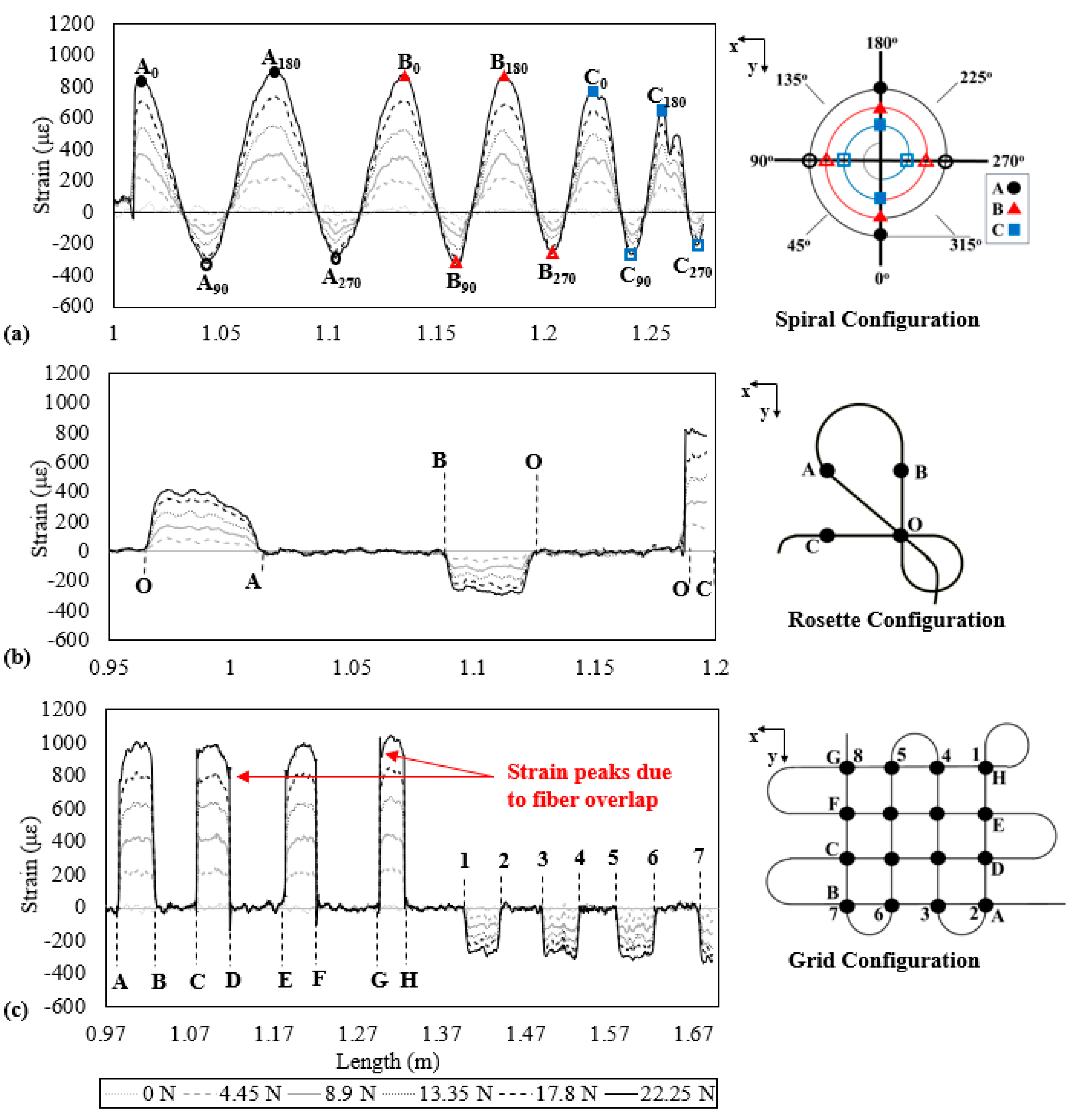
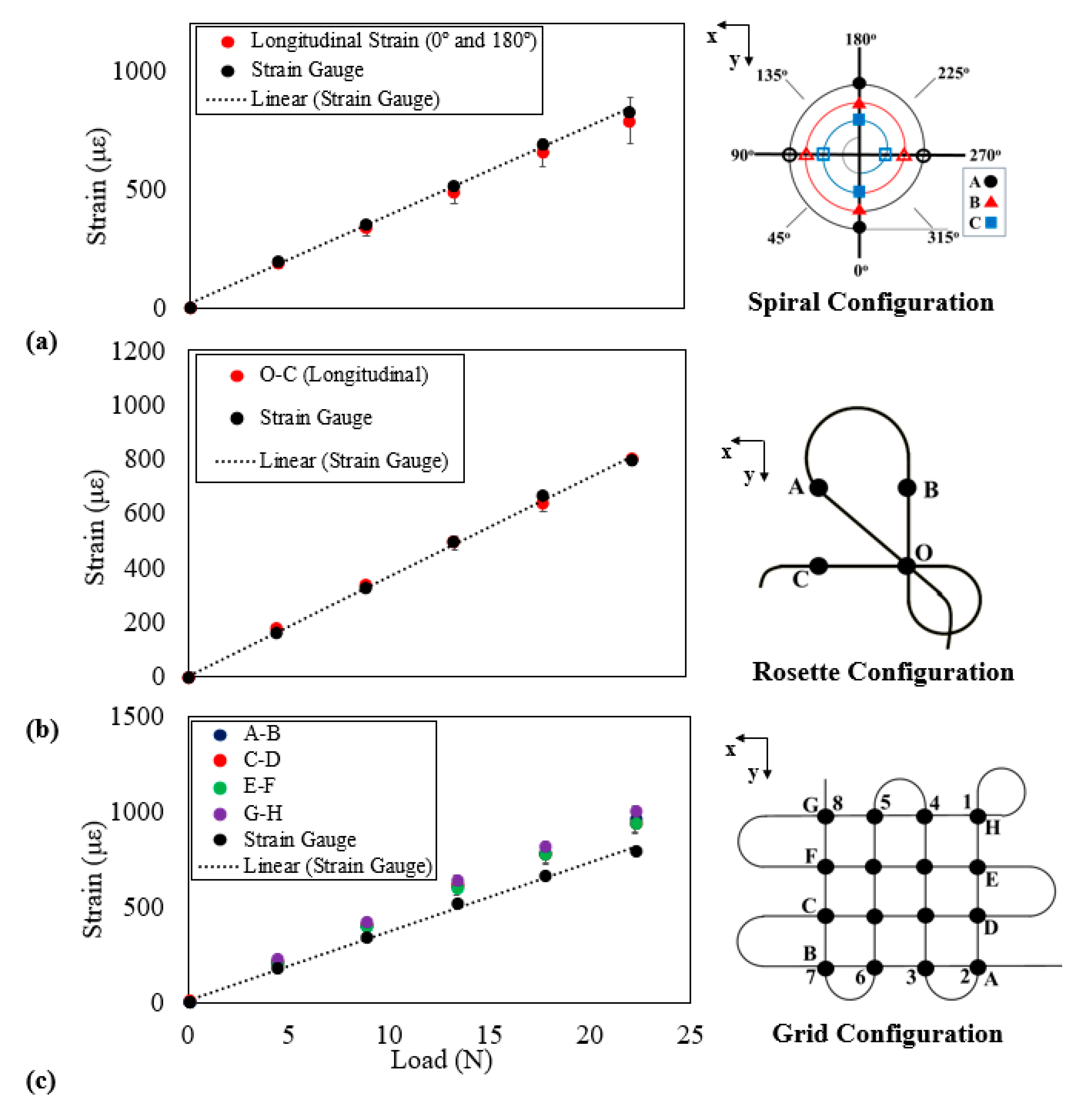
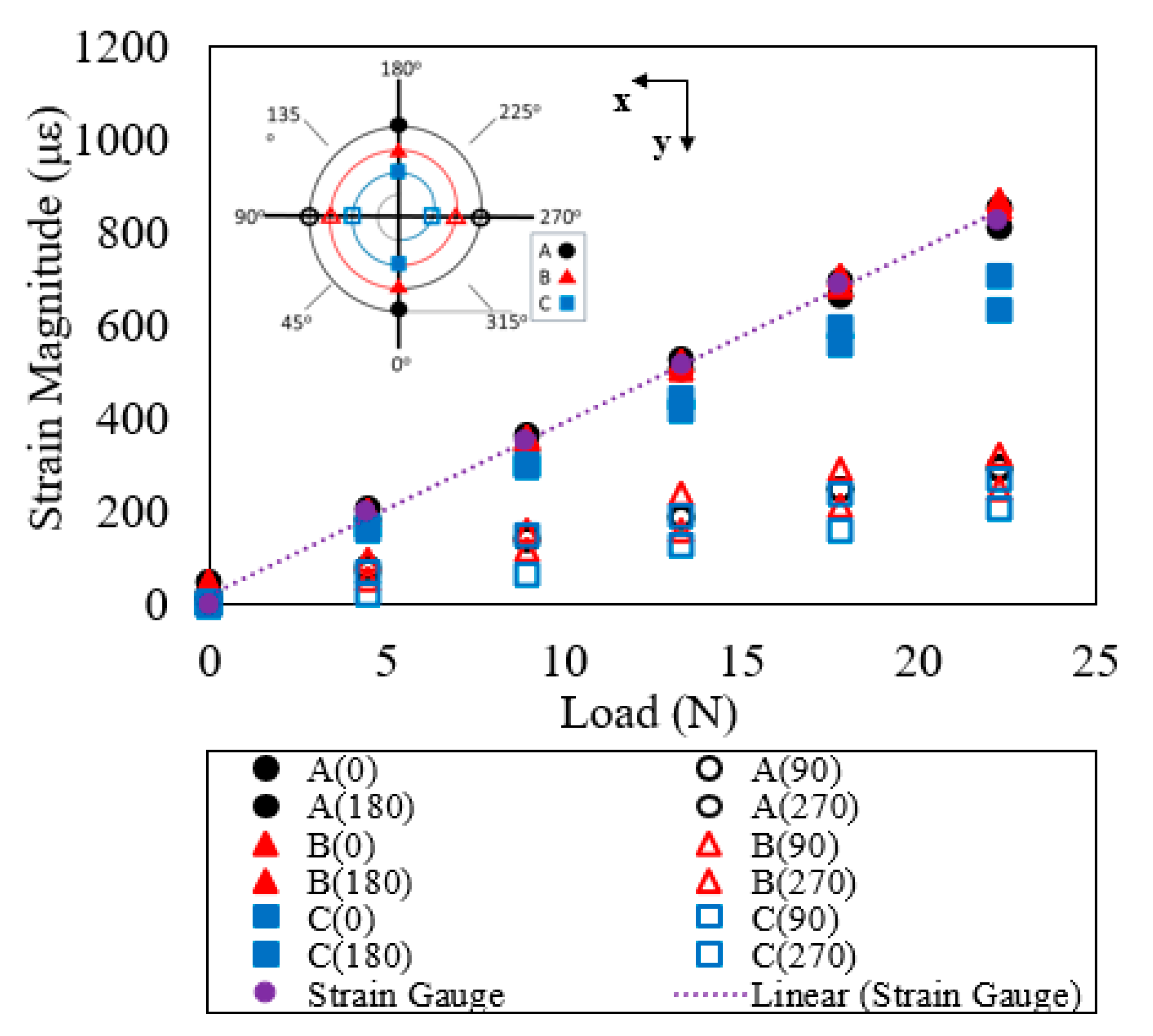
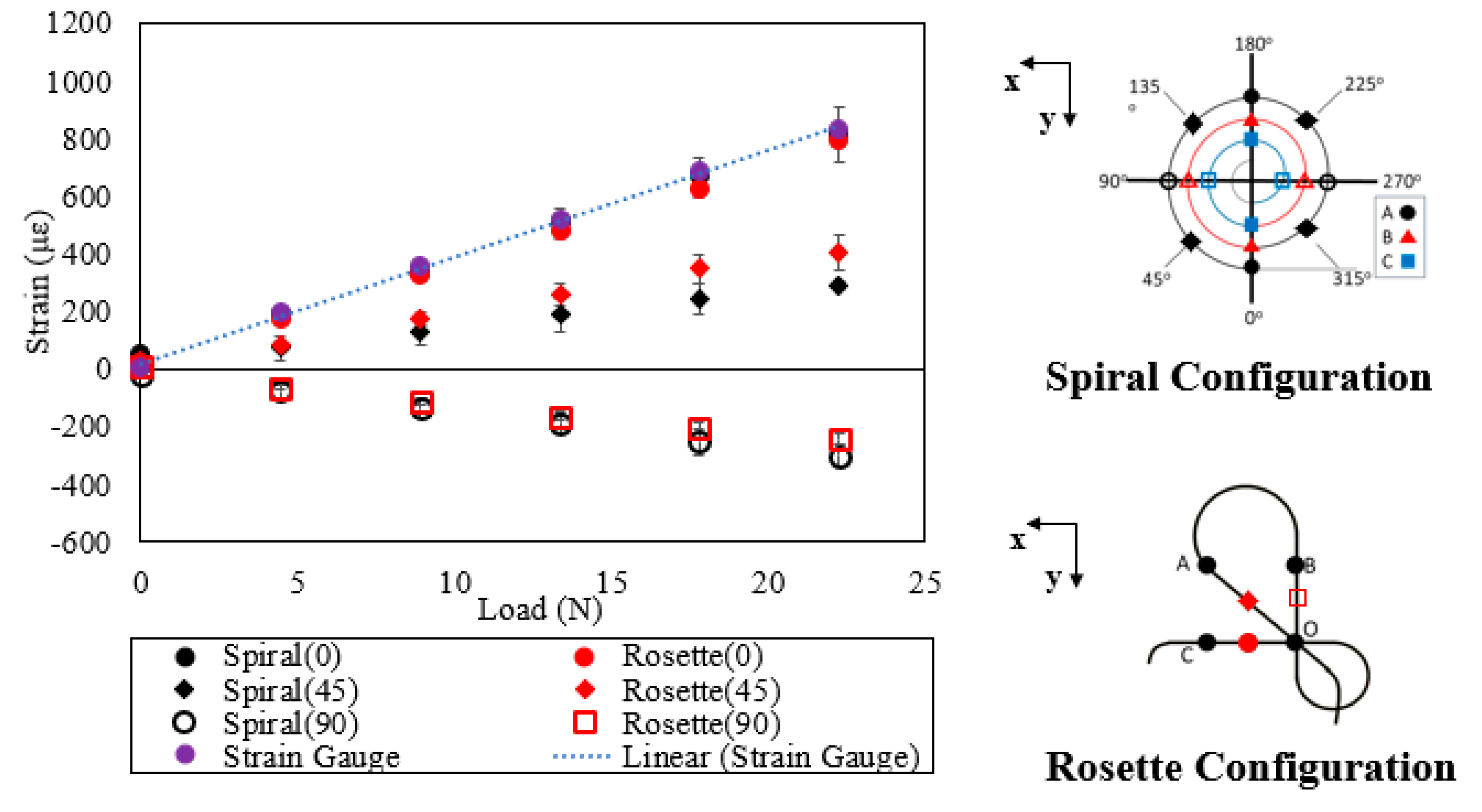
| Spiral | OF | 186.8 | 337.7 | 488.8 | 653.5 | 789.2 |
| SG | 196.0 | 356.0 | 517.0 | 686.0 | 829.0 | |
| % Diff | 4.7 | 5.2 | 5.5 | 4.7 | 4.8 | |
| Rosette | OF | 172.8 | 335.6 | 492.4 | 636.3 | 797.0 |
| SG | 158.0 | 323.0 | 493.0 | 662.0 | 791.0 | |
| % Diff | 9.4 | 3.9 | 0.1 | 3.9 | 0.8 | |
| Grid | OF | 212.4 | 407.2 | 614.0 | 785.4 | 957.1 |
| SG | 175.0 | 338.0 | 510.0 | 655.0 | 798.0 | |
| % Diff | 21.4 | 20.5 | 20.4 | 19.9 | 19.9 | |
© 2018 by the authors. Licensee MDPI, Basel, Switzerland. This article is an open access article distributed under the terms and conditions of the Creative Commons Attribution (CC BY) license (http://creativecommons.org/licenses/by/4.0/).
Share and Cite
Drake, D.A.; Sullivan, R.W.; Wilson, J.C. Distributed Strain Sensing from Different Optical Fiber Configurations. Inventions 2018, 3, 67. https://doi.org/10.3390/inventions3040067
Drake DA, Sullivan RW, Wilson JC. Distributed Strain Sensing from Different Optical Fiber Configurations. Inventions. 2018; 3(4):67. https://doi.org/10.3390/inventions3040067
Chicago/Turabian StyleDrake, Daniel A., Rani W. Sullivan, and J. Caleb Wilson. 2018. "Distributed Strain Sensing from Different Optical Fiber Configurations" Inventions 3, no. 4: 67. https://doi.org/10.3390/inventions3040067
APA StyleDrake, D. A., Sullivan, R. W., & Wilson, J. C. (2018). Distributed Strain Sensing from Different Optical Fiber Configurations. Inventions, 3(4), 67. https://doi.org/10.3390/inventions3040067