Robust Multi-Output Prediction of Perovskite Solar Cell Parameters via Multi-Task Learning

Abstract

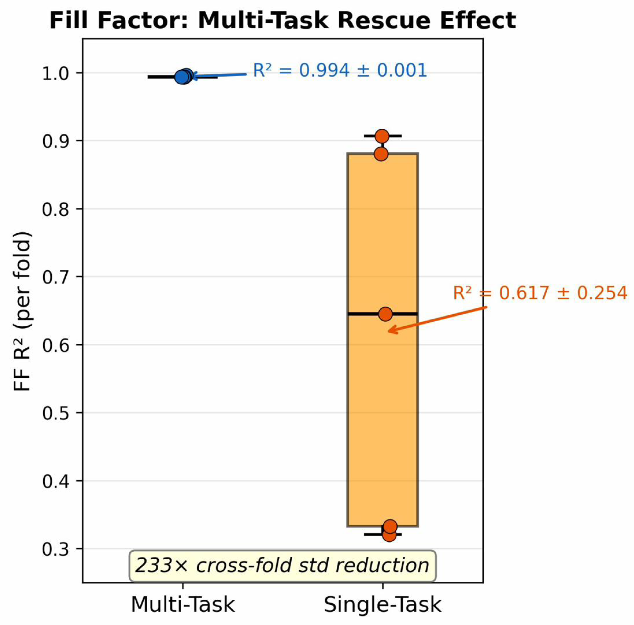
Conventional machine learning models for perovskite solar cells predict photovoltaic parameters independently, disregarding the physical constraint $\mathrm{PCE}=V_{oc}\times J_{sc}\times \mathrm{FF}/100$. This approach can yield mutually incompatible predictions for the four parameters, a failure mode that has not been hitherto quantified in the perovskite solar cell literature. This paper proposes a multi-head neural network with a shared backbone, physics-guided feature construction, and task-specific prediction heads, and validates it on 7176 SCAPS-1D simulations across 12 perovskite compositions. When benchmarked against architecturally matched single-task baselines, the multi-task model, optimized via 5-fold cross-validation, achieves $R^2$ values of at least 0.994 for all four targets, with cross-fold standard deviations of 0.001. In particular, fill factor prediction improves from $R^2=0.617\pm 0.254$ (single-task) to $0.994\pm 0.001$ (multi-task), a 233-fold reduction in cross-fold standard deviation. Application of a physical consistency metric developed in this work reveals that 36.5% of single-task predictions exceed a 2 PCE-unit implausibility threshold, compared to only 0.01% for the multi-task model. The multi-task model outperforms the single-task baseline in all 20-fold target comparisons, with large effect sizes (Cohen’s $d=1.33$–$8.93$). These results confirm multi-task learning as an effective approach for achieving robust, stable, and internally consistent predictions in simulation-based photovoltaic virtual screening.

1. Introduction

Perovskite solar cells (PSCs) are promising candidates in next-generation photovoltaics, with power conversion efficiencies surpassing 26% [1,2]. The compositional and architectural design space of these cells is rather broad, as it encompasses diverse cation–halide combinations, charge-transport layers, and device geometries. Conventional experimental approaches are too slow to explore this space systematically [3,4]. As a consequence, machine learning (ML) has become essential for PSC development, as it enables screening thousands of candidate architectures in silico prior to physical synthesis and validation [5,6].

The performance of solar cells is characterized by four parameters: open-circuit voltage ($V_{oc}$), short-circuit current density ($J_{sc}$), fill factor (FF), and power conversion efficiency (PCE). These are related through the following formula:

$$\mathrm{PCE}={\displaystyle \frac{V_{oc}\times J_{sc}\times \mathrm{FF}}{100}}$$

(1)

Current ML approaches for PSCs predict these parameters independently. This gives rise to a problem that extends beyond inaccuracy: four individually plausible predictions may be mutually inconsistent. Consider a virtual screening pipeline that predicts a PCE of 25% alongside $V_{oc}$, $J_{sc}$, and FF values whose product yields only 18%, a physically impossible configuration. For ML-assisted virtual screening to be reliable, the predicted parameters must be both individually accurate and physically consistent, i.e., they must approximately satisfy Equation (1). However, to the authors’ knowledge, no prior study has proposed a metric to quantify inter-parameter consistency in PSC prediction or assessed whether multi-task learning improves performance.

It is important to note that since PCE is algebraically determined by $V_{oc}$, $J_{sc}$, and FF via Equation (1), any model that predicts these three parameters with sufficient accuracy will yield consistent PCE predictions as a by-product, regardless of whether the model explicitly shares representations. The consistency metric introduced in this work should therefore be understood as a diagnostic tool for detecting prediction failures rather than as evidence that the model has learned underlying device physics.

1.1. Prior Work

In the literature, the application of ML to predict perovskite solar cell performance has been the subject of growing interest [7,8]. On the one hand, several studies focus on predicting PCE alone. Novoselov et al. [9], for instance, applied CatBoost to 7182 SCAPS-1D configurations and achieved high PCE accuracy. However, models that predict only PCE cannot identify whether underperformance stems from low voltage, poor current collection, or resistance losses, as they do not provide $V_{oc}$, $J_{sc}$, or FF estimates. On the other hand, studies that do predict all four parameters treat them independently. Reza et al. [10] used Random Forest with SHAP analysis on 1000 simulated Rb₂SnBr₆ configurations, Li et al. [11] combined Extra Trees with Bayesian optimization on 847 experimental samples, and Saidani et al. [12] applied neural networks for Rb₂ScCuCl₆-based PSCs. Yet, none of these studies verified whether the four predicted parameters satisfy Equation (1). A further shared limitation of the aforementioned studies is the reliance on single compositions or small datasets, which calls into question the generalizability of the reported findings.

The present work addresses three gaps arising from these limitations. First, no PSC-ML study in the literature has implemented multi-task learning with a shared backbone for simultaneous parameter prediction. Second, no formally defined metric exists to quantify the physical consistency among predicted parameters. Third and finally, prediction stability across cross-validation folds has not been evaluated through statistical significance testing.

Table 1. Comparison with prior ML approaches for PSC parameter prediction.

Reference	Method	Data Source	Samples	Compositions	Targets	Consistency
Novoselov [9]	CatBoost	SCAPS-1D	7182	12	PCE only	No
Reza [10]	Rand. Forest	SCAPS-1D	1000	1	4 (indep.)	No
Li [11]	Extra Trees	Experim.	847	Multiple	Per-output	No
Saidani [12]	NN + SHAP	SCAPS-1D	—	1	Per-output	No
This work	MH-NN (MTL)	SCAPS-1D	7176	12	4 (joint)	Yes

Note: Direct $R^2$ comparison across studies is confounded by differences in dataset size, compositional diversity, and model class. The contribution of this work is the multi-task architecture and consistency evaluation framework, not absolute accuracy.

summarizes how this work is positioned relative to existing studies.

1.2. Multi-Task Learning Background

Multi-task learning (MTL) is a training paradigm that enhances generalization by training a single model on multiple related tasks simultaneously [13]. In the hard-parameter-sharing approach adopted in this work, a shared backbone network extracts features common to all tasks, while task-specific heads branch from this shared representation to produce individual outputs. The shared backbone acts as an inductive bias that regularizes the model against overfitting to any single target. This is particularly relevant when certain targets are harder to predict, as gradient information from other tasks can stabilize the learning of such targets.

MTL has been successfully applied in related materials science domains. Li et al. [14], for instance, employed multi-task learning to jointly forecast battery capacity and power degradation and reported improvements in both accuracy and computational cost over single-task approaches. Multi-task frameworks have also been used to predict multiple material properties simultaneously in high-throughput computational studies, where the outputs are physically coupled [15]. However, to the authors’ knowledge, MTL has not been applied to the simultaneous prediction of PSC parameters, and its potential to promote physical consistency between predicted outputs remains unexplored.

1.3. Contributions

We summarize our main contributions in the following four points.

First, we propose a multi-head neural network with physics-guided feature construction using six domain-knowledge features and task-specific head depths calibrated to physical complexity. The architecture is validated through ablation studies and baseline benchmarking on 7176 SCAPS-1D configurations across 12 perovskite compositions.

Second, we show that multi-task learning affords cross-fold stability guarantees that single-task approaches do not achieve. In particular, FF prediction improves from $R^2=0.617\pm 0.254$, with individual folds as low as $R^2=0.32$, to $R^2=0.994\pm 0.001$, a 233-fold reduction in cross-fold standard deviation. The multi-task model achieves higher $R^2$ values than the single-task baseline across all 20-fold target comparisons.

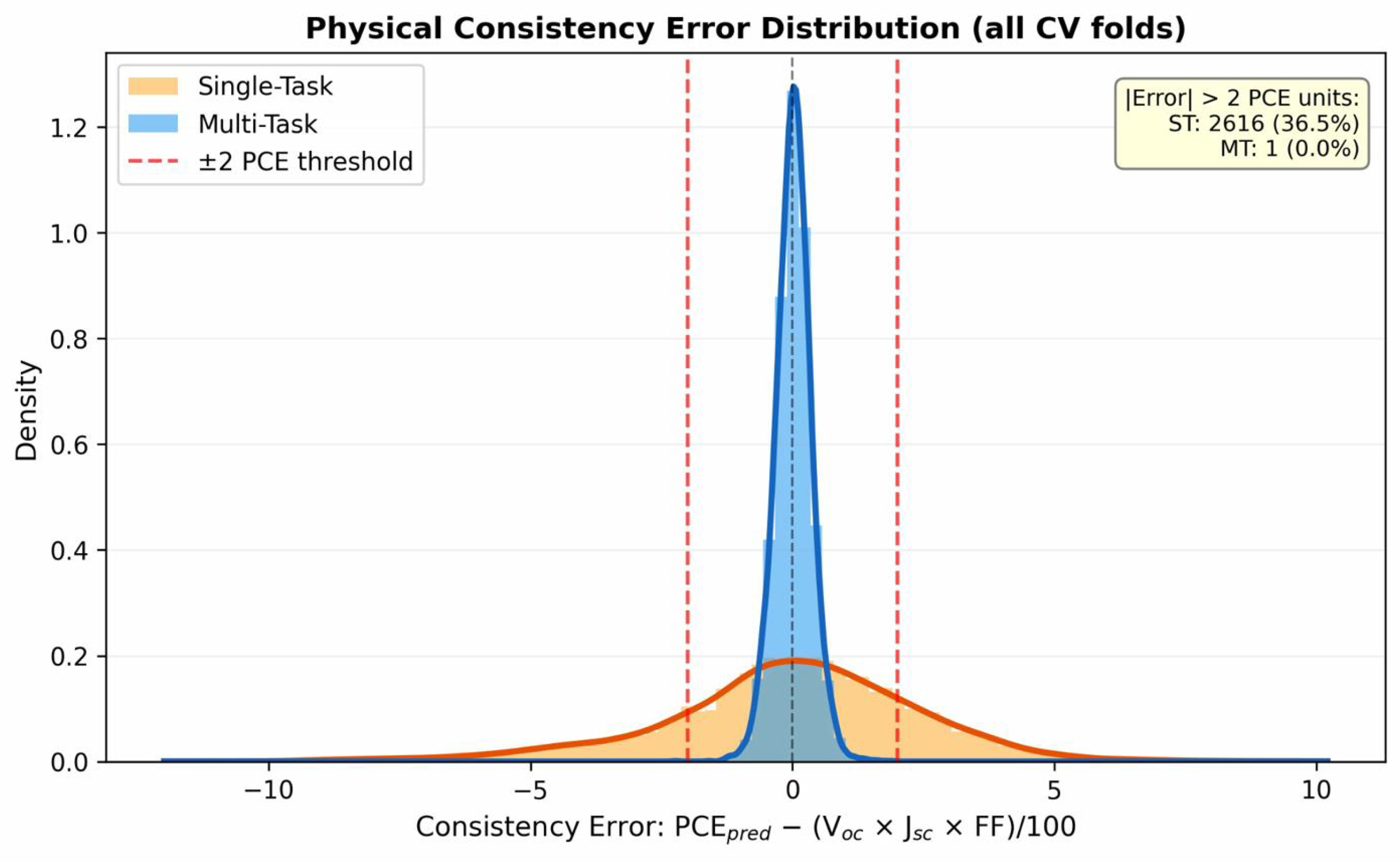
Third, we introduce a metric for quantifying inter-parameter consistency in multi-output PSC prediction. The metric is defined as the deviation between the predicted PCE and the product $V_{oc,\mathrm{pred}}\times J_{sc,\mathrm{pred}}\times {\mathrm{FF}}_{\mathrm{pred}}/100$, with a threshold of 2 PCE units to flag physically implausible predictions. Application of this metric reveals that 36.5% of single-task predictions are physically implausible, compared to only 0.01% for multi-task predictions, a failure mode not captured by per-target $R^2$ alone.

Fourth, SHapley Additive exPlanations (SHAP)-based analysis confirms that the model captures the statistical correlations present in the SCAPS-1D simulation outputs, including the halide-mediated $V_{oc}$–$J_{sc}$ trade-off, the thickness–$J_{sc}$ Beer–Lambert relationship, and ETL-dominated PCE control.

The rest of the paper is organized as follows. Section 2 describes the dataset and physics-guided feature construction, presents the model architecture and training protocol and details the experimental design. Section 3 reports results on prediction accuracy, consistency, ablation studies, baseline comparisons, and interpretability. Section 4 discusses the mechanisms underlying the multi-task advantage and its limitations. Finally, Section 5 concludes the work.

2. Materials and Methods

2.1. Dataset and Feature Construction

This section describes the dataset and the preprocessing and feature engineering strategies adopted to prepare the data for multi-output prediction. Particular attention is given to the construction of physics-guided features, which encode domain knowledge of perovskite solar cell operation into the input space. This allows the model to exploit established physical relationships before the learning process begins.

2.1.1. SCAPS-1D Simulation Dataset

The dataset used in this work was generated by Novoselov et al. [9] using SCAPS-1D, a one-dimensional solar cell simulation tool that solves coupled Poisson and continuity equations under drift-diffusion transport [16]. SCAPS-1D is widely used in the photovoltaics community for modeling the performance of thin-film solar cells under idealized conditions.

The original dataset comprises 7182 device configurations obtained by systematically varying perovskite compositions, electron transport layer (ETL) and hole transport layer (HTL) materials, absorber layer thickness, fluorine-doped tin oxide (FTO) substrate presence, and device polarity. Simulations were performed under standard AM1.5G illumination at 300 K. For each configuration, four photovoltaic parameters were recorded: $V_{oc}$, $J_{sc}$, FF, and PCE. Outliers were removed using a Z-score threshold of $\left|Z\right|>4$ for any target variable, resulting in 7176 retained configurations.

The dataset includes 12 distinct perovskite compositions: three pure-cation compounds (CsPbI₃, N = 1008; MAPbI₃, $N=1001$; FAPbI₃, $N=903$) and nine mixed-cation formulations with varying Cs, MA, and FA stoichiometries ($N=350$–974 per composition). All compositions employ the I/Br halide system. The absorber thickness was varied from 200 to 800 nm. Device configurations feature eight ETL types (indexed 1–8), eleven HTL types (indexed 1–11), the presence or absence of an FTO conductive substrate, and both n-i-p and p-i-n device polarities.

Table 2. Target variable distributions ($N=7176$).

Target	Min	Max	Mean	Std	Median	N
$V_{oc}$ (V)	0.934	2.005	1.309	0.228	1.243	7176
$J_{sc}$ (mA/cm2)	2.488	28.500	17.670	7.644	20.544	7176
FF (%)	14.759	90.876	73.692	14.658	81.685	7176
PCE (%)	2.154	30.988	16.517	7.621	17.780	7176

summarizes the distributions of the target variables.

The use of simulation data is a deliberate methodological choice. SCAPS-1D outputs are deterministic functions of their inputs and do not include measurement noise. As a consequence, the high $R^2$ values reported in Section 3.3 are partly attributable to this smooth manifold, and lower $R^2$ values would be expected on experimental data subject to measurement noise and unmodeled physical effects. This choice is intentional: simulation data isolates the question of whether multi-task learning improves prediction stability and promotes inter-parameter consistency from confounding experimental noise. The transferable finding is the relative advantage of multi-task over single-task baselines, as both are evaluated on the same data under identical conditions.

2.1.2. Input Feature Processing

The initial input space consists of six continuous and four categorical variables. The continuous features are the perovskite absorber thickness (Pero_th) and five compositional fractions representing A-site and X-site occupancy (Cs, MA, FA for the cation site; I, Br for the halide site). These features were standardized using Z-score normalization, with parameters calculated independently within each cross-validation fold to prevent information leakage. The four categorical features, i.e., ETL type, HTL type, FTO presence, and device polarity, were encoded using one-hot encoding with the drop-first convention to mitigate multicollinearity. Following encoding, the categorical features expand to 17 binary indicators. The resulting feature space comprises 6 continuous, 17 one-hot encoded, and 6 engineered features described in the following section, totaling 29 input features.

2.1.3. Physics-Guided Feature Construction

In contrast to physics-informed neural networks, which incorporate governing partial differential equations directly into the loss function [17], the present approach introduces domain knowledge at the input level through physically motivated feature transformations. We refer to this as physics-guided feature construction. It provides the model with precomputed representations of established physical interactions, thereby reducing its reliance on raw inputs to infer these relationships. Six engineered features were developed based on domain expertise in perovskite photovoltaics.

Table 3. Physics-guided engineered features.

Feature	Formula	Physical Justification
Cs × MA	Cs · MA	A-site cation interaction: non-linear mixing effects on lattice stability and bandgap
I × Br	I · Br	Halide interaction: mixed-halide effects on absorption edge and defect chemistry
Cs/FA	Cs/(FA + $\epsilon$)	Cation ratio: governs tolerance factor and phase stability
I/Br	I/(Br + $\epsilon$)	Halide ratio: controls bandgap via valence band maximum; primary $V_{oc}$–$J_{sc}$ trade-off
Optical Depth	Pero_th2	Quadratic thickness: Beer–Lambert absorption gain saturation
Vol. Recomb.	Pero_th × (MA + FA)	Thickness–composition interaction: volumetric recombination scaling

presents each feature, its formula, and the physical rationale for its inclusion.

Ratio features are constrained to the range $[0,10]$, with $\epsilon ={10}^{-8}$ added to the denominator to prevent numerical instability as FA or Br approach zero. The contribution of these features is evaluated in the ablation study of Section 3.1. The complete 29-feature set improves consistency, as measured by mean absolute error, by 8.3% compared to the original 23-feature set (0.254 versus 0.277), while $R^2$ values remain comparable.

We emphasize the distinction between physics-guided and physics-informed approaches. The present work is physics-guided: domain knowledge is used to construct input features (e.g., the I/Br ratio, Cs/FA ratio, optical depth) that encode established physical relationships before training begins. The model itself is a standard neural network with no physics-based constraints in the loss function or architecture. This contrasts with physics-informed approaches (e.g., PINNs), which embed governing equations directly into the training objective. The consistency observed in this work is therefore emergent from the shared-backbone architecture and high prediction accuracy, not enforced by physical constraints.

2.2. Model Architecture and Training

This section describes the neural network architecture and training protocol developed for the simultaneous prediction of four photovoltaic parameters. We first introduce the multi-head architecture consisting of a shared backbone and task-specific heads. We then describe the loss weighting strategy, the training protocol, and the construction of architecturally matched single-task baselines that allow us to isolate the effect of multi-task learning.

2.2.1. Multi-Head Neural Network Architecture

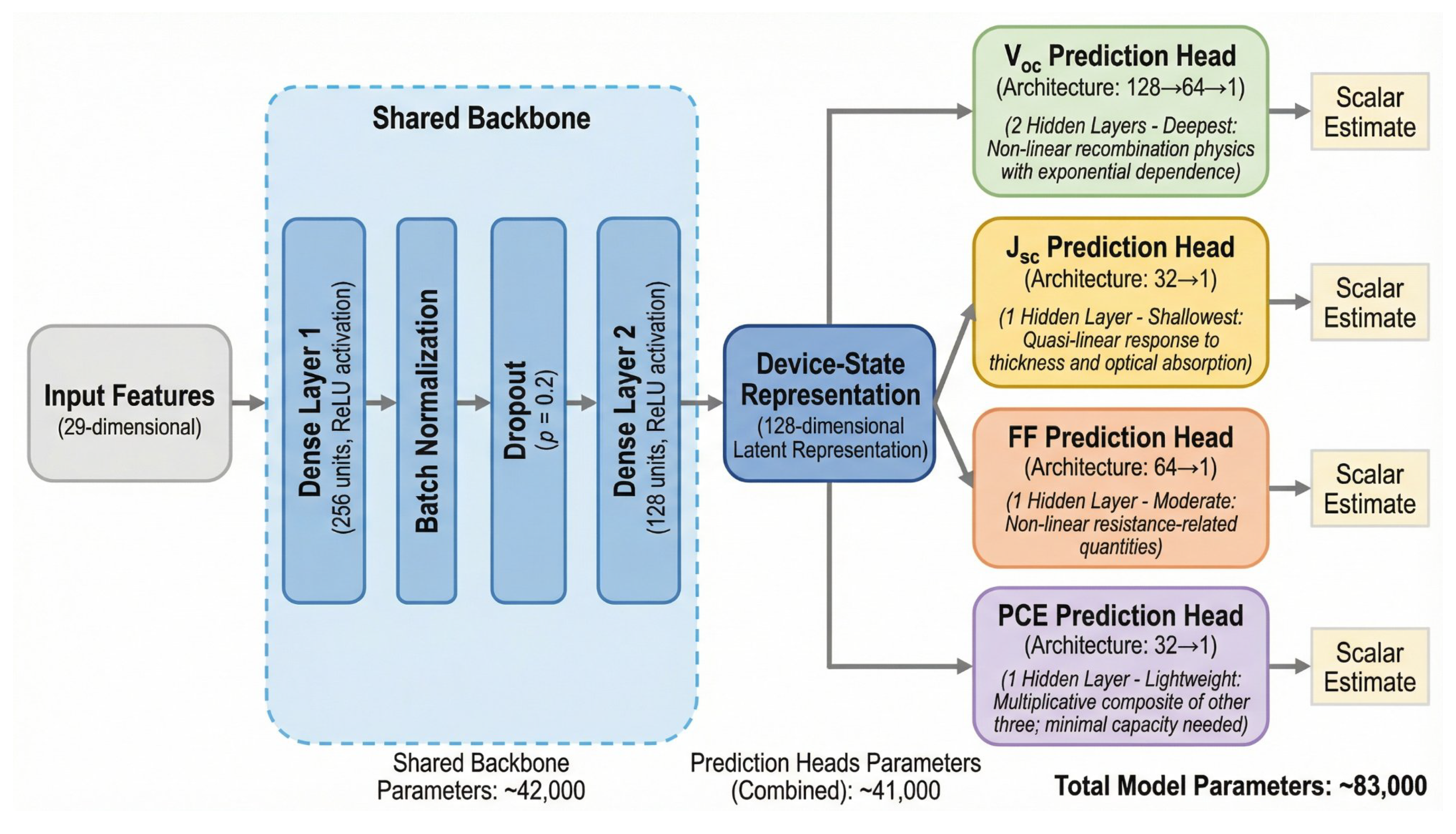
The proposed model adopts a hard-parameter-sharing architecture in which a shared backbone transforms the input features into a common latent representation. Four task-specific prediction heads then branch from this representation to produce scalar estimates of $V_{oc}$, $J_{sc}$, FF, and PCE.

The backbone consists of two fully connected layers. The first contains 256 units with ReLU activation, followed by batch normalization [18] and dropout at a rate of $p=0.2$ [19]. The second contains 128 units with ReLU activation. This compresses the 29-dimensional input to a 128-dimensional latent vector, hereafter referred to as the device-state representation. Four independent heads then map this vector to each target. The depth of each head is calibrated according to the physical complexity of its target, as summarized in

Table 4. Task-specific head configurations.

Target	Architecture	Hidden Layers	Physical Rationale
$V_{oc}$	128 → 64 → 1	2 (deepest)	Non-linear recombination physics with exponential dependence
$J_{sc}$	32 → 1	1 (shallowest)	Quasi-linear response to thickness and optical absorption
FF	64 → 1	1 (moderate)	Non-linear resistance-related quantities
PCE	32 → 1	1 (lightweight)	Multiplicative composite of the other three; minimal capacity needed

.

The complete multi-task model contains approximately 83,000 trainable parameters, of which 42,000 are allocated to the shared backbone, and 41,000 are distributed among the four heads. In comparison, a single-task baseline consists of the backbone and one head; training four independent single-task models yields a total of approximately 206,000 parameters. Figure 1 illustrates the architecture.

2.2.2. Loss Function and Weighting Strategy

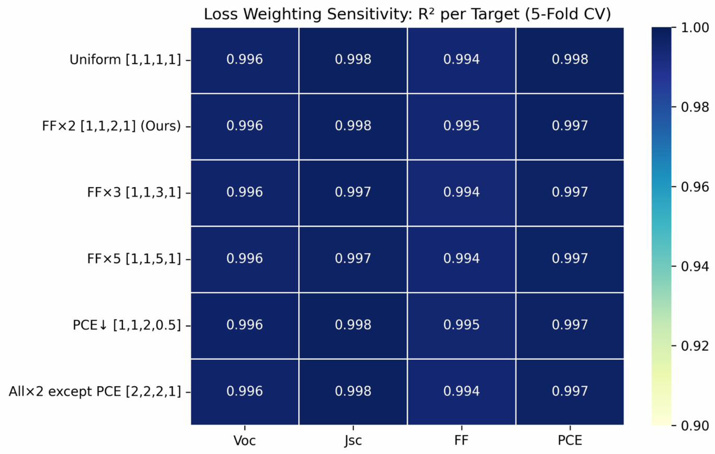
The multi-task model is trained by minimizing a weighted sum of per-target MSE losses, with weights $\lambda =[1.0,1.0,2.0,1.0]$. FF receives double weight owing to its being the most difficult target for single-task models: it exhibits the highest cross-fold standard deviation (standard deviation = 0.254 in single-task $R^2$) and the lowest mean single-task $R^2$ (0.617). Section 3.2 examines the sensitivity of model performance to the choice of loss weights. It is worth noting that $R^2$ varies by less than 0.002 across the six tested configurations, which suggests that performance is not sensitive to the selected weights within the tested range. Alternative weighting strategies, such as homoscedastic uncertainty weighting [20], are identified as a direction for future research.

2.2.3. Training Protocol

All models are trained using the AdamW optimizer [21] with an initial learning rate of ${10}^{-3}$ and MSE loss. The training budget is 200 epochs, although early stopping with a patience of 15 epochs on validation loss consistently halts training before this limit. The learning rate is reduced on plateau by a factor of 0.5 with a patience of 7 epochs. The mini-batch size is 64 samples. To prevent state leakage across models, each training run uses newly instantiated callback objects for early stopping and learning rate scheduling.

2.2.4. Single-Task Baseline Design

To isolate the effect of multi-task learning, we establish an architecturally matched single-task baseline. Four separate neural networks are trained, one per target, each replicating the backbone and head architecture of the corresponding branch in the multi-task model. The training protocol, i.e., optimizer, learning rate schedule, early stopping, batch size, and epoch budget, is identical across all models. The only difference between the multi-task and single-task configurations is whether the backbone parameters are updated on the basis of one task or all four simultaneously. This design ensures that any observed performance difference is attributable solely to the multi-task paradigm and not to differences in model capacity or training procedure.

2.3. Experimental Design

This section presents the experimental framework used to evaluate the proposed multi-task model. We first describe the cross-validation protocol, then introduce a physical consistency metric to assess the plausibility of predictions, and finally specify the statistical tests used for performance comparison. The ablation studies and baseline comparisons that contextualize the contribution of the multi-task approach are outlined at the end of the section.

2.3.1. Cross-Validation Protocol

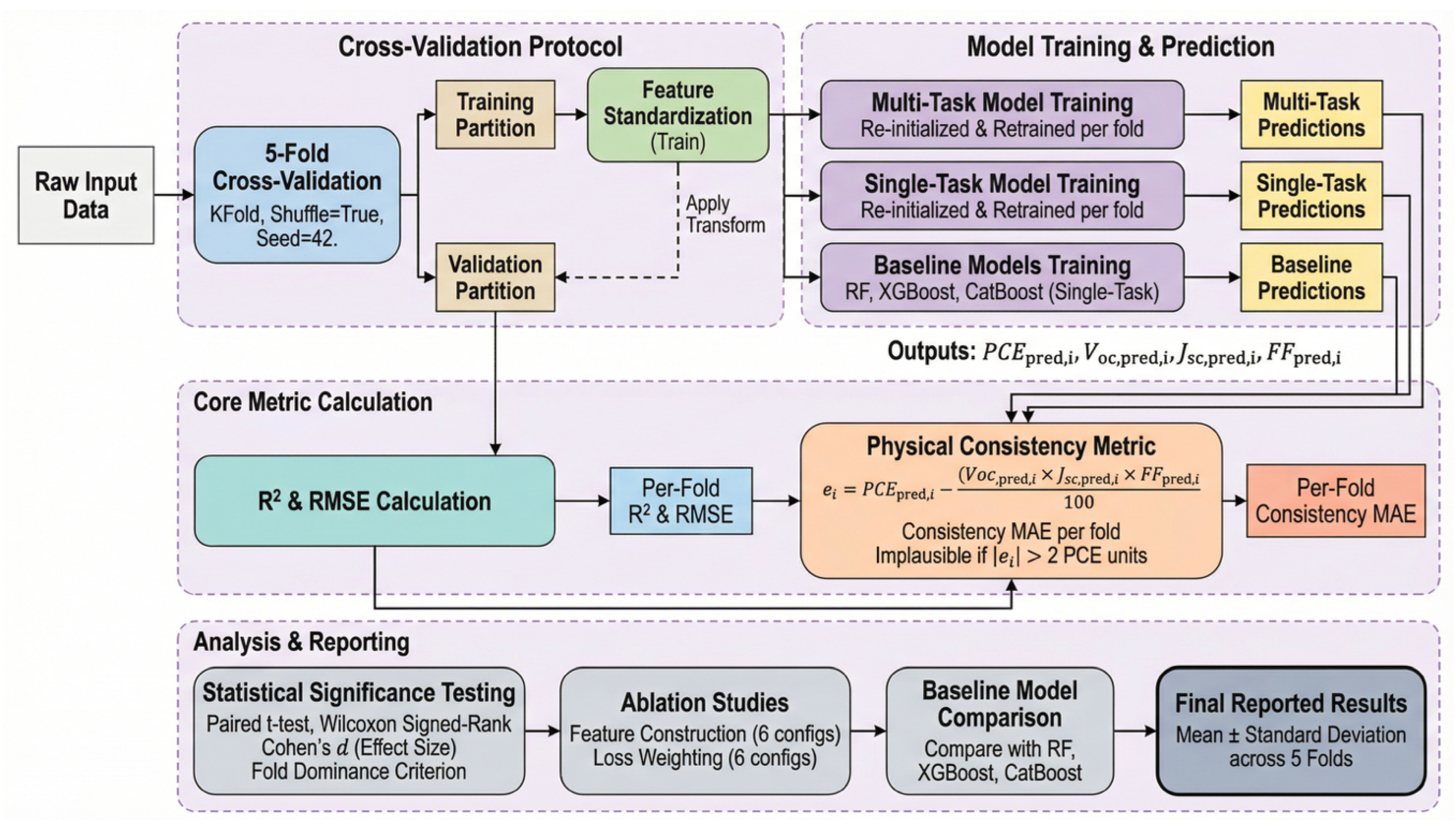
All experiments employ 5-fold cross-validation with shuffling enabled and a random seed of 42. For each fold, feature standardization parameters are calculated on the training partition and applied to the validation partition to prevent information leakage. Both multi-task and single-task models are re-initialized and retrained from scratch for every fold. $R^2$ and RMSE are recorded per target per fold, and results are reported as the mean and standard deviation across the five folds.

2.3.2. Physical Consistency Metric

We introduce a metric that quantifies the extent to which the four predicted parameters adhere to the fundamental relationship in Equation (1). For each test sample i, the signed consistency error is defined as:

$$e_i={\mathrm{PCE}}_{\mathrm{pred},i}-{\displaystyle \frac{V_{oc,\mathrm{pred},i}\times J_{sc,\mathrm{pred},i}\times {\mathrm{FF}}_{\mathrm{pred},i}}{100}}$$

(2)

The consistency error is aggregated as a per-fold MAE. Predictions for which $|e_i|$ exceeds 2 PCE units are classified as physically implausible. This threshold corresponds to a relative mismatch of approximately 10 to 15% for typical mid-range devices (PCE ≈ 15–20%). To the authors’ knowledge, no such metric has been proposed in the perovskite solar cell ML literature.

2.3.3. Statistical Significance Testing

A paired t-test and a Wilcoxon signed-rank test are conducted on the per-fold $R^2$ values, and effect size is quantified using Cohen’s d. Note that for $n=5$ folds, the minimum attainable Wilcoxon p-value is 0.0625 (two-sided). A qualitative fold-dominance criterion is also reported, indicating whether the multi-task model achieves a higher $R^2$ in every fold for every target.

2.3.4. Ablation Studies

Two ablation studies are conducted. The first, presented in Section 3.1, assesses the contribution of physics-guided features using a leave-one-group-out protocol across six configurations. The second, in Section 3.2, examines the sensitivity of model performance to task-specific loss weights across six weight configurations.

2.3.5. Baseline Model Selection

Three additional baselines are evaluated: Random Forest with hyperparameters optimized via nested 3-fold grid search [10], XGBoost [22] with tuned hyperparameters, and CatBoost [23] with default hyperparameters (iterations = 500, depth = 7, learning rate = 0.05) as implemented by Novoselov et al. [9]. All tree-based baselines are trained in single-task mode, with one model per target, as these methods do not inherently support hard parameter sharing. The physical consistency metric is applied to their four independent predictions to allow a direct comparison. Figure 2 provides an overview of the experimental design.

3. Results

This section presents the results obtained from applying the multi-task learning framework to the SCAPS-1D dataset. We first examine the contribution of physics-guided features and the sensitivity to loss weighting, and then compare the multi-task and single-task architectures in terms of physical consistency and prediction accuracy. We continue with baseline comparisons, statistical validation, and subgroup analyses, and conclude with interpretability studies that shed light on the physical relationships recovered by the model.

3.1. Feature Construction Ablation

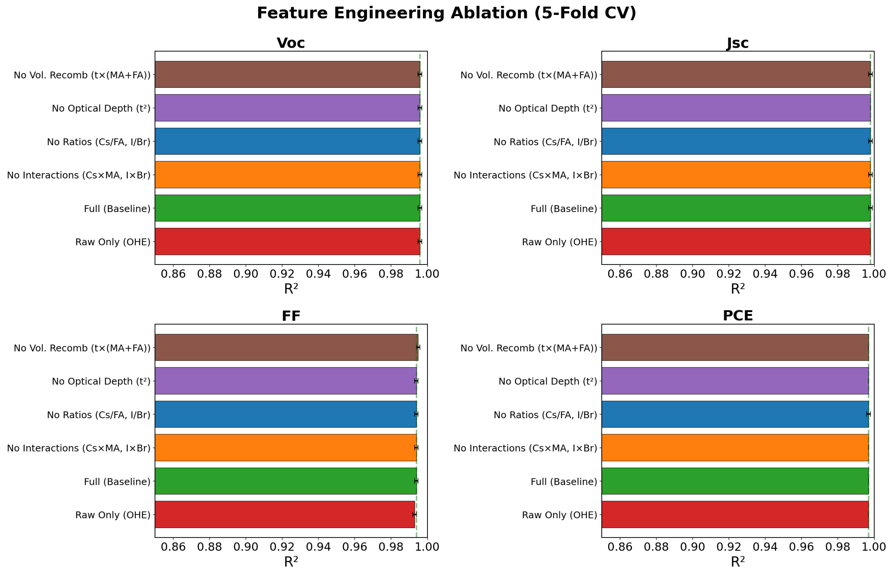
For feature ablation,

Table 5. Feature construction ablation (multi-task model, 5-fold CV).

Configuration	${\mathit{V}}_{\mathit{oc}}$${\mathit{R}}^2$	${\mathit{J}}_{\mathit{sc}}$${\mathit{R}}^2$	FF ${\mathit{R}}^2$	PCE ${\mathit{R}}^2$	Cons. MAE
Raw Only (23 feat.)	$0.996\pm 0.001$	$0.997\pm 0.001$	$0.994\pm 0.001$	$0.997\pm 0.001$	0.277
Full (29 feat.)	$0.996\pm 0.001$	$0.998\pm 0.001$	$0.994\pm 0.001$	$0.997\pm 0.000$	0.254
No Interactions	$0.996\pm 0.001$	$0.998\pm 0.001$	$0.994\pm 0.001$	$0.997\pm 0.000$	0.253
No Ratios	$0.996\pm 0.001$	$0.998\pm 0.000$	$0.994\pm 0.001$	$0.997\pm 0.000$	0.256
No Optical Depth	$0.996\pm 0.001$	$0.998\pm 0.001$	$0.995\pm 0.001$	$0.997\pm 0.000$	0.246
No Vol. Recomb.	$0.996\pm 0.001$	$0.998\pm 0.000$	$0.995\pm 0.001$	$0.997\pm 0.000$	0.238

and Figure 3 show that $R^2$ remains stable across all six feature configurations, varying by at most 0.001 for any target. This stability indicates that the multi-task architecture, rather than the specific feature set, is the primary driver of prediction accuracy. In contrast, the consistency MAE reveals a meaningful differentiation, where the complete 29-feature set achieves a consistency MAE of 0.254, an 8.3% improvement over the raw 23-feature configuration (0.277). This improvement stems entirely from enhanced inter-parameter coherence rather than from gains in per-target accuracy.

The leave-one-group-out analysis yields an unexpected result. Excluding the volumetric recombination feature (Pero_th × (MA + FA)) improves consistency MAE from 0.254 to 0.238, the best among all configurations. Similarly, removing the optical depth feature (Pero_th²) yields a consistency MAE of 0.246. These findings suggest that although physics-motivated features encode genuine physical interactions, they may introduce subtle redundancies with information already captured by the shared backbone, giving rise to minor interference with the optimization. The interaction features (Cs × MA, I × Br) and ratio features (Cs/FA, I/Br) have negligible individual impact on consistency (0.253 and 0.256, respectively), which indicates that consistency gains arise from the collective representational capacity of the feature set rather than from any single engineered feature.

These results indicate that while the full set of six physics-guided features improves consistency, some features are individually redundant. Optical depth (Pero_th²) and the volumetric recombination proxy (Pero_th × (MA + FA)) overlap with information already captured by the raw thickness and composition inputs. Feature redundancy does not harm $R^2$ in this setting but contributes marginally to consistency through the compositional ratio features (Cs/FA, I/Br), which provide the model with precomputed representations of physically relevant relationships.

3.2. Loss Weighting Sensitivity

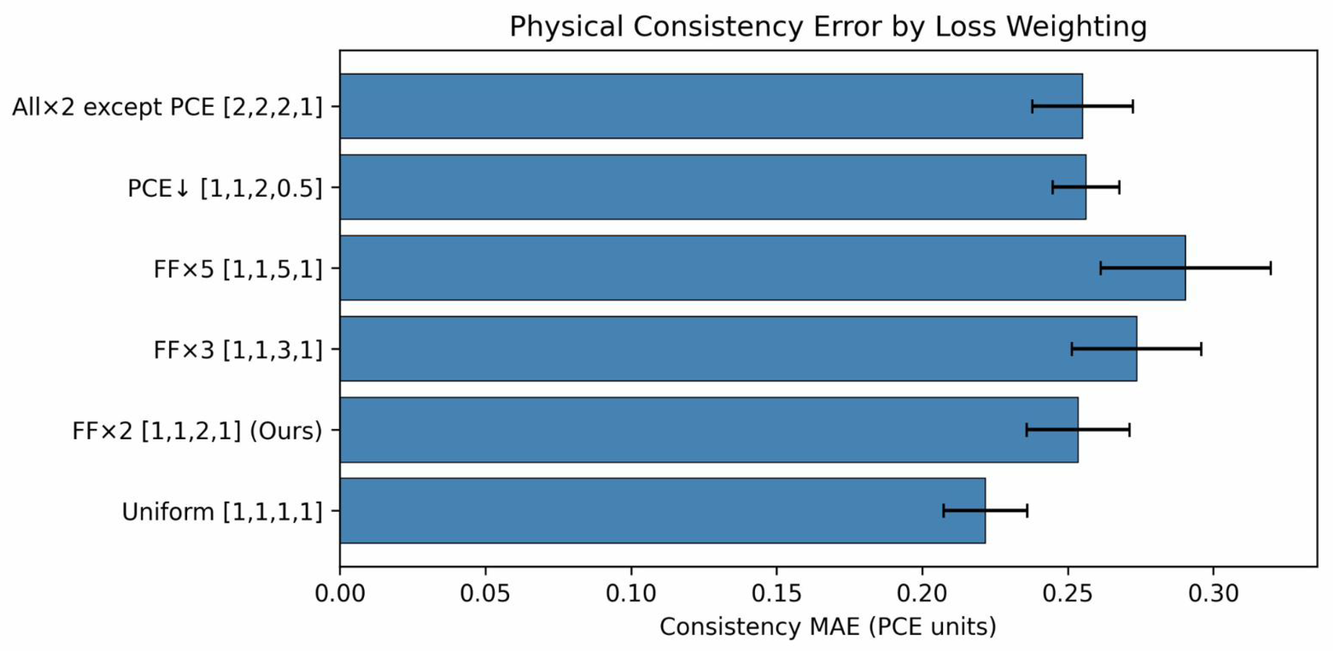
$R^2$ varies by at most 0.001 across all six weight configurations (

Table 6. Loss weighting sensitivity (5-fold CV).

Config	${\mathit{V}}_{\mathit{oc}}$${\mathit{R}}^2$	${\mathit{V}}_{\mathit{oc}}$ RMSE	${\mathit{J}}_{\mathbf{sc}}$${\mathit{R}}^2$	${\mathit{J}}_{\mathbf{sc}}$ RMSE	FF ${\mathit{R}}^2$	FF RMSE	PCE ${\mathit{R}}^2$	Cons. MAE
$[1,1,1,1]$	0.996	0.014	0.998	0.353	0.994	1.117	0.998	0.222
$[1,1,2,1]$ *	0.996	0.014	0.998	0.377	0.995	1.084	0.997	0.254
$[1,1,3,1]$	0.996	0.015	0.997	0.397	0.994	1.124	0.997	0.274
$[1,1,5,1]$	0.996	0.015	0.997	0.407	0.994	1.097	0.997	0.291
$[1,1,2,0.5]$	0.996	0.014	0.998	0.362	0.995	1.057	0.997	0.256
$[2,2,2,1]$	0.996	0.014	0.998	0.356	0.994	1.113	0.997	0.255

* Chosen configuration. Loss weight order: $[{\lambda }_{V_{oc}},{\lambda }_{J_{sc}},{\lambda }_{\mathrm{FF}},{\lambda }_{\mathrm{PCE}}]$.

, Figure 4), confirming that prediction accuracy is robust to the choice of loss weights. However, the consistency MAE reveals a trade-off not captured by $R^2$ alone. Uniform weighting $[1,1,1,1]$ yields the lowest consistency MAE (0.222), whereas increasing the FF emphasis progressively degrades this metric: 0.254 at FF × 2, 0.274 at FF × 3, and 0.291 at FF × 5 (Figure 5). This monotonic decline indicates that overweighting a single task distorts the shared backbone representation, improving that task at the expense of inter-parameter coherence.

The RMSE values corroborate this observation. The FF RMSE reaches its minimum at the $[1,1,2,0.5]$ configuration (1.057) rather than at the highest FF weight, while $J_{sc}$ RMSE increases steadily from 0.353 (uniform) to 0.407 (FF × 5). This suggests that excessive FF weighting diverts representational capacity from other targets. The selected configuration $[1,1,2,1]$ constitutes a balanced compromise: it achieves the highest FF $R^2$ (0.995) and the lowest FF RMSE (1.084) among configurations with practical utility, while maintaining an acceptable consistency of 0.254.

3.3. Cross-Validated Prediction Accuracy

The most notable result is the improvement in FF prediction, as illustrated in

Table 7. 5-fold CV prediction accuracy (multi-task vs. single-task neural network).

Target	MT ${\mathit{R}}^2$ (Mean ± Std)	ST ${\mathit{R}}^2$ (Mean ± Std)	$\mathbf{\Delta }{\mathit{R}}^2$	Cohen’s d
$V_{oc}$	$0.996\pm 0.001$	$0.961\pm 0.009$	$+0.035$	3.58
$J_{sc}$	$0.998\pm 0.001$	$0.963\pm 0.018$	$+0.035$	1.72
FF	$0.994\pm 0.001$	$0.617\pm 0.254$	$+0.377$	1.33
PCE	$0.997\pm 0.001$	$0.872\pm 0.014$	$+0.125$	8.93

and Figure 6. In the single-task setting, FF $R^2$ ranges from 0.321 (Fold 3) to 0.907 (Fold 2), with a standard deviation of 0.254, which is a level of instability that is incompatible with deployment. Multi-task learning eliminates this instability entirely through stabilizing FF at $R^2=0.994\pm 0.001$ and reducing the cross-fold standard deviation by a factor of 233.

The per-fold $R^2$ values expose the limitations of single-task models more clearly than aggregate statistics. For $V_{oc}$, single-task $R^2$ ranges from 0.947 to 0.971; for $J_{sc}$, from 0.938 to 0.984; for PCE, from 0.856 to 0.894. Although all targets experience reduced single-task performance, only FF demonstrates severe collapse in specific folds. This fold-dependent failure is not apparent from the mean $R^2$ and poses a risk for deployment: a model that appears adequate on average may produce highly inaccurate predictions on certain data partitions. It is worth noting that the multi-task model outperforms the single-task baseline in every fold for every target, achieving 20 out of 20 pairwise wins. This consistent superiority affords stronger evidence than statistical significance testing alone, as it demonstrates improvement without relying on distributional assumptions.

3.4. Physical Consistency Analysis

The per-fold consistency analysis in

Table 8. Per-fold consistency MAE (PCE units).

Model	Fold 1	Fold 2	Fold 3	Fold 4	Fold 5	Mean
Multi-Task	0.249	0.232	0.303	0.269	0.266	0.264
Single-Task	2.002	1.412	2.424	2.235	1.279	1.871
Ratio (ST/MT)	8.0×	6.1×	8.0×	8.3×	4.8×	7.1×

shows a consistent 5- to 8-fold advantage for the multi-task model across all five folds. The multi-task consistency MAE ranges from 0.232 to 0.303, spanning 0.071 PCE units. The single-task consistency MAE, in contrast, ranges from 1.279 to 2.424, spanning 1.145 PCE units. There is a direct relationship between FF collapse and consistency degradation: the worst single-task consistency occurs in Fold 3 (MAE = 2.424), which is the fold where single-task FF $R^2$ drops to 0.321. Similarly, Fold 4 (consistency MAE = 2.235) corresponds to FF $R^2=0.332$. The two folds with the best single-task consistency (Folds 2 and 5, MAE = 1.412 and 1.279) are those with the highest single-task FF $R^2$ (0.907 and 0.880).

The threshold analysis, as shown in

Table 9. Physical consistency threshold analysis (multi-task vs. single-task).

Model	Cons. MAE	Std	Fraction > 2 PCE-Unit Threshold
Multi-Task	0.264	0.343	0.014% (1 sample)
Single-Task	1.871	2.487	36.5% (2616 samples)

and Figure 7, exposes the most pronounced difference. The multi-task model produces virtually no physically implausible predictions: only 1 out of 7176 samples (0.014%) exceeds the 2 PCE-unit threshold. In the single-task case, 2616 predictions (36.5%) exceed this threshold. In these cases, the four predicted parameters are mutually incompatible, i.e., they correspond to device configurations that cannot physically exist, even though each parameter appears reasonable when evaluated by per-target $R^2$. This failure mode has not been previously identified in the PSC-ML literature and constitutes a risk for deployment in virtual screening pipelines that has been hitherto overlooked.

3.5. Baseline Model Comparisons

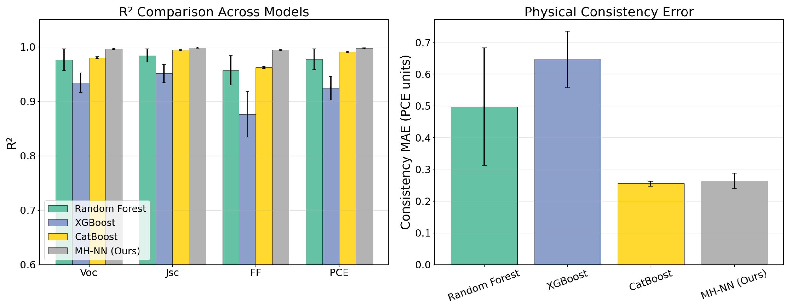
The MH-NN achieves the highest $R^2$ across all targets (

Table 10. Full baseline comparison (5-fold CV).

Model	${\mathit{V}}_{\mathit{oc}}$${\mathit{R}}^2$	${\mathit{J}}_{\mathit{sc}}$${\mathit{R}}^2$	FF ${\mathit{R}}^2$	PCE ${\mathit{R}}^2$	Cons. MAE
Random Forest	$0.976\pm 0.020$	$0.984\pm 0.012$	$0.957\pm 0.027$	$0.977\pm 0.019$	$0.497\pm 0.185$
XGBoost	$0.934\pm 0.018$	$0.951\pm 0.017$	$0.876\pm 0.042$	$0.924\pm 0.022$	$0.646\pm 0.089$
CatBoost	$0.980\pm 0.002$	$0.994\pm 0.001$	$0.962\pm 0.002$	$0.991\pm 0.001$	$0.255\pm 0.008$
MH-NN (Ours)	$0.996\pm 0.001$	$0.998\pm 0.001$	$0.994\pm 0.001$	$0.997\pm 0.001$	$0.264\pm 0.024$

, Figure 8) with the lowest cross-fold variability. Among the tree-based baselines, CatBoost is the strongest, with $R^2\ge 0.962$ for all targets and low variance (standard deviation $\le 0.002$). Random Forest attains robust accuracy but exhibits higher variance (standard deviation = 0.012–0.027). XGBoost is the weakest, particularly on FF ($R^2=0.876\pm 0.042$), which confirms that FF prediction is the most challenging target across model classes.

CatBoost achieves a consistency MAE of $0.255\pm 0.008$, nearly identical to the MH-NN’s $0.264\pm 0.024$. This result warrants examination. On a smooth, noise-free simulation manifold where individual predictions are accurate ($R^2\ge 0.962$ for CatBoost), physical consistency arises arithmetically: if each parameter is predicted within approximately 1% error, the PCE computed from those predictions will closely match the directly predicted PCE. High individual accuracy is therefore sufficient for consistency on clean data, without shared representations.

This observation redefines the role of the consistency metric. It does not serve to distinguish MH-NN from CatBoost on simulation data. Rather, it functions as a diagnostic tool that reveals the catastrophic inconsistency of single-task neural networks, which produce 36.5% physically implausible predictions. Two factors distinguish the MH-NN for practical applications. First, its FF $R^2$ (0.994) surpasses CatBoost’s (0.962) by 0.032, a gap that is likely to widen on noisier experimental data. Second, in scenarios where individual accuracy is unreliable, as the single-task neural network results demonstrate, shared representations provide a structural safeguard against consistency collapse.

3.6. Statistical Significance

All paired t-tests in

Table 11. Statistical significance testing (multi-task vs. single-task neural network).

Target	MT ${\mathit{R}}^2$	ST ${\mathit{R}}^2$	Paired t p	Wilcoxon p	Cohen’s d
$V_{oc}$	0.996	0.961	0.001	0.063	3.58
$J_{sc}$	0.998	0.963	0.018	0.063	1.72
FF	0.994	0.617	0.041	0.063	1.33
PCE	0.997	0.872	<0.001	0.063	8.93

are statistically significant at $\alpha =0.05$, with p-values ranging from <0.001 (PCE) to 0.041 (FF). The Wilcoxon signed-rank test yields $p=0.0625$ for all targets, which is the minimum attainable value with $n=5$ paired observations and reflects the mathematical constraint of small-sample non-parametric tests rather than a lack of significance. Cohen’s d values are consistently large, with a range from 1.33 to 8.93. Each of these values exceeds the conventional threshold for a large effect ($d>0.8$) by a factor of 1.7 to 11.2.

The PCE result ($d=8.93$) indicates that the per-fold $R^2$ distributions are separated by nearly nine pooled standard deviations. The FF result ($d=1.33$), although the smallest, is influenced by the high single-task variance (standard deviation = 0.254); the actual $R^2$ gap ($\Delta =0.377$) is the largest among all targets. The fold dominance criterion provides the strongest evidence: the multi-task model achieves a higher $R^2$ in every fold for every target, i.e., 20 out of 20 comparisons without exception.

3.7. Subgroup Analysis

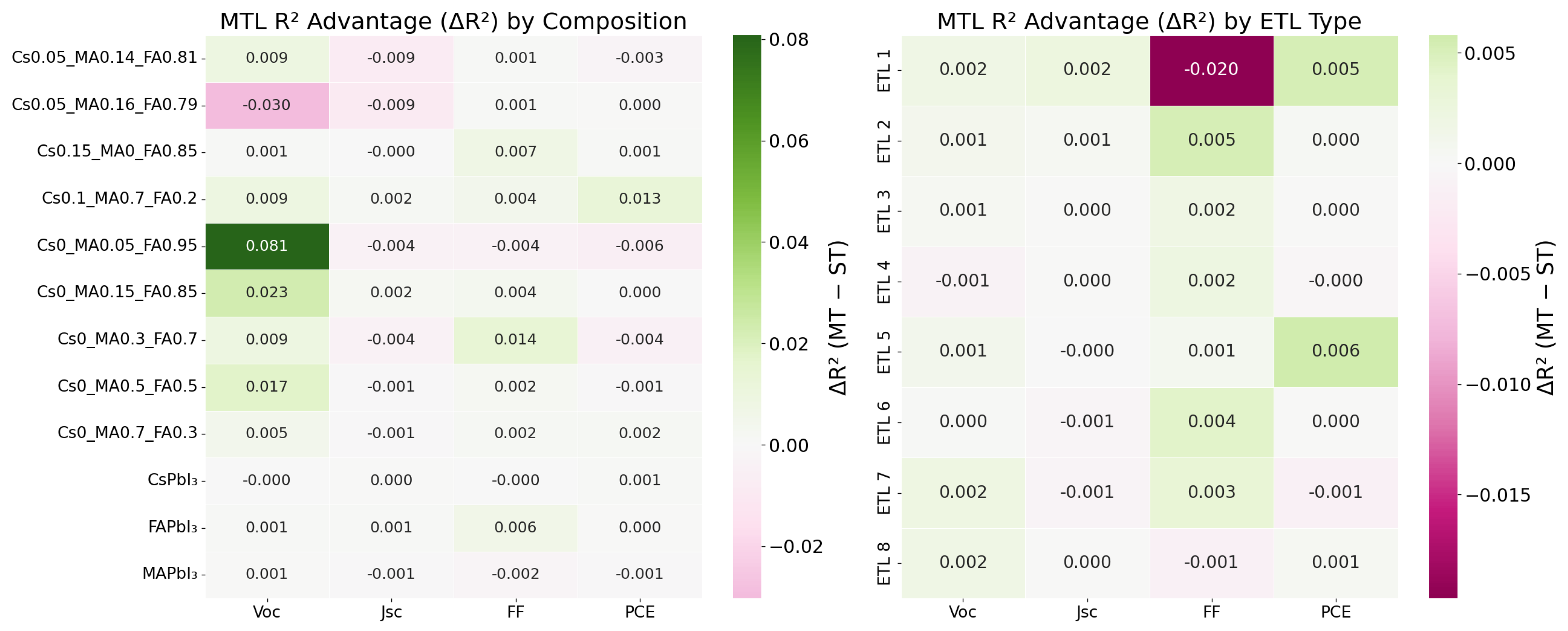
Per-composition analysis reported in

Table 12. Per-composition $\Delta R^2$ (MT − ST) and sample sizes.

Composition	N	${\mathit{V}}_{\mathit{oc}}$$\mathbf{\Delta }{\mathit{R}}^2$	${\mathit{J}}_{\mathit{sc}}$$\mathbf{\Delta }{\mathit{R}}^2$	FF $\mathbf{\Delta }{\mathit{R}}^2$	PCE $\mathbf{\Delta }{\mathit{R}}^2$	Note
CsPbI3	1008	−0.000	+0.000	−0.000	+0.001	Largest comp.
MAPbI3	1001	+0.001	−0.001	−0.002	−0.001
FAPbI3	903	+0.001	+0.001	+0.006	+0.000
Cs0.15FA0.85	974	+0.001	−0.000	+0.007	+0.001
Cs0MA0.05FA0.95	420	+0.081	−0.004	−0.004	−0.006	Largest $V_{oc}$ gain
Cs0.1MA0.7FA0.2	490	+0.009	+0.002	+0.005	+0.013	Lowest $J_{sc}$ $R^2$
Cs0MA0.3FA0.7	420	+0.009	−0.004	+0.014	−0.004	Largest FF gain
Cs0MA0.15FA0.85	560	+0.023	+0.002	+0.004	+0.000
Cs0MA0.5FA0.5	350	+0.017	−0.001	+0.002	−0.001
Cs0MA0.7FA0.3	350	+0.005	−0.001	+0.002	+0.002
Cs0.05MA0.14FA0.81	350	+0.009	−0.009	+0.001	−0.003
Cs0.05MA0.16FA0.79	350	−0.030	−0.009	+0.001	+0.000	Only $V_{oc}$ regression

N denotes the total number of samples for each composition in the full dataset.

and Figure 9 shows that among 48 composition–target comparisons, 29 exhibit positive $\Delta R^2$, 18 are negative, and 1 is zero. The mean absolute $\Delta R^2$ is 0.006, an order of magnitude smaller than the aggregate improvements in Table 7. The largest positive gain is for Cs₀MA_0.05FA_0.95 on $V_{oc}$ ($\Delta R^2=+0.081$), while the only notable regression is for Cs_0.05MA_0.16FA_0.79 on $V_{oc}$ ($\Delta R^2=-0.030$). No composition shows consistent degradation across all four targets. The mixed directionality and small effect sizes support the conclusion that the aggregate multi-task improvements stem from fold-level stabilization via cross-task gradient sharing rather than from composition-specific accuracy gains.

The three pure-cation compositions (CsPbI₃, MAPbI₃, FAPbI₃), which account for 41% of the dataset, exhibit near-zero $\Delta R^2$ across all targets ($|\Delta R^2| \le 0.006$). These compositions have the largest sample sizes (903–1008) and are therefore well represented in all folds. The multi-task advantage is most pronounced for smaller, mixed-cation compositions where fold-to-fold representational variation is greatest, an observation that is consistent with the interpretation that cross-task regularization is the driving mechanism.

The per-ETL analysis (

Table 13. Per-ETL $\Delta R^2$ (MT − ST) by electron transport layer.

ETL	${\mathit{N}}_{\mathbf{test}}$	${\mathit{V}}_{\mathit{oc}}$$\mathbf{\Delta }{\mathit{R}}^2$	${\mathit{J}}_{\mathit{sc}}$$\mathbf{\Delta }{\mathit{R}}^2$	FF $\mathbf{\Delta }{\mathit{R}}^2$	PCE $\mathbf{\Delta }{\mathit{R}}^2$	Mean $|\mathbf{\Delta }{\mathit{R}}^2|$
1	77	+0.002	+0.002	−0.020	+0.005	0.007
2	226	+0.001	+0.001	+0.005	+0.000	0.002
3	212	+0.001	+0.000	+0.002	+0.000	0.001
4	223	−0.001	+0.000	+0.002	−0.000	0.001
5	133	+0.001	−0.000	+0.001	+0.006	0.002
6	219	+0.000	−0.001	+0.004	+0.000	0.001
7	215	+0.002	−0.001	+0.003	−0.001	0.002
8	131	+0.002	+0.000	−0.001	+0.001	0.001

$N_{\mathrm{test}}$ denotes the number of test-fold samples for each subgroup.

) provides independent corroborating evidence. Across 32 ETL–target comparisons, the mean absolute $\Delta R^2$ is 0.002, even lower than the per-composition value of 0.006. Both models achieve $R^2>0.94$ for each ETL and target, confirming that neither model encounters difficulties with specific transport-layer chemistries. The largest per-ETL effect is a negative $\Delta R^2$ for ETL₁ on FF ($-0.020$), where the multi-task model marginally underperforms ($R^2=0.955$ vs. 0.975). ETL₁ has the smallest sample size ($N_{\mathrm{test}}=77$), which likely accounts for this outcome owing to representational trade-offs in the shared backbone. Even in this least favorable case, the multi-task FF $R^2$ of 0.955 remains high.

3.8. Feature Importance and Interpretability

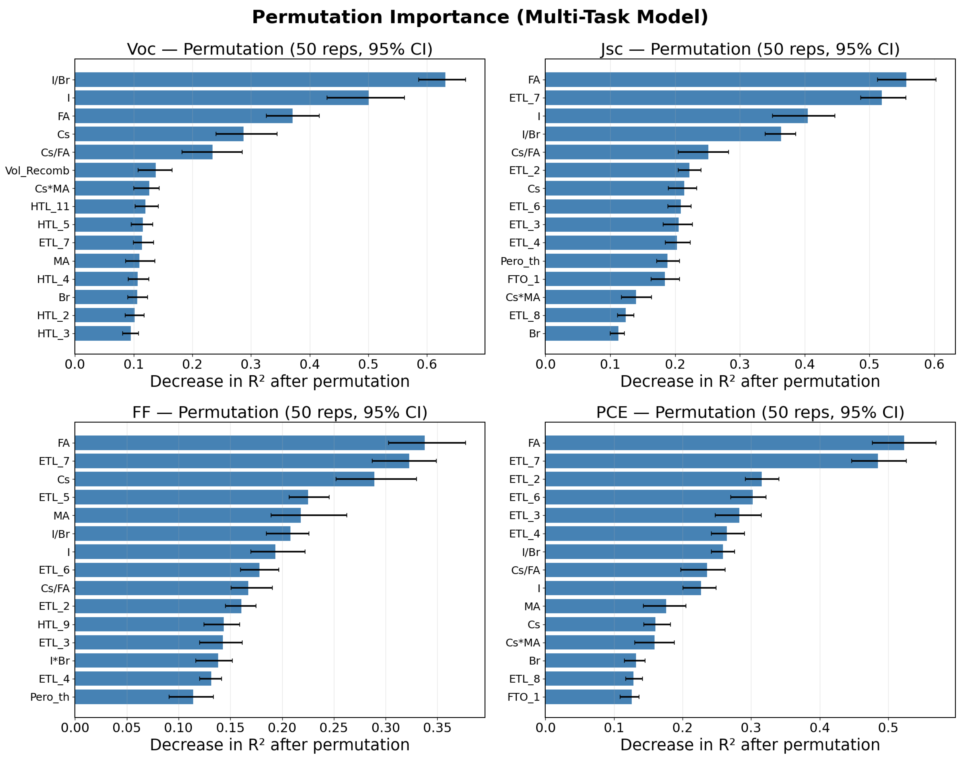
Permutation importance analysis (

Table 14. Permutation importance (top 10 features, 50 repetitions).

Feature	${\mathit{V}}_{\mathit{oc}}$ Imp.	${\mathit{J}}_{\mathit{sc}}$ Imp.	FF Imp.	PCE Imp.
I/Br (ratio)	0.631	0.364	0.208	0.259
FA	0.371	0.557	0.338	0.523
I	0.501	0.405	0.194	0.227
ETL7	0.114	0.519	0.323	0.485
Cs	0.287	0.214	0.289	0.160
Cs/FA (ratio)	0.235	0.251	0.167	0.236
ETL2	0.041	0.222	0.161	0.315
ETL6	0.044	0.209	0.178	0.302
ETL3	0.039	0.205	0.143	0.283
MA	0.110	0.099	0.218	0.176

, Figure 10) reveals a target-dependent feature hierarchy that is consistent with established perovskite photovoltaic physics. Three observations are noteworthy.

First, the I/Br ratio is the most influential predictor for $V_{oc}$, with an importance of 0.631, nearly double its importance for any other target. The iodide fraction (I) is the second most significant feature for $V_{oc}$ (0.501). These values indicate that the model has identified the primary mechanism governing $V_{oc}$ in mixed-halide perovskites: halide composition determines the bandgap, which sets $V_{oc}$ according to the Shockley–Queisser limit. The comparatively lower importance of I/Br for $J_{sc}$ (0.364) and FF (0.208) reflects the fact that these targets are governed by distinct physical mechanisms.

Second, the FA fraction is the dominant feature for both $J_{sc}$ (0.557) and PCE (0.523), consistent with the established role of formamidinium in optimizing the bandgap and absorption coefficient in the visible spectrum. The high importance of FA for PCE, surpassing even the I/Br ratio (0.259), suggests an indirect influence through both the $J_{sc}$ and FF pathways. The Cs/FA ratio (importance 0.235–0.251) captures the competition between cesium and formamidinium for A-site occupancy, which is associated with tolerance factor and phase stability.

Third, several ETL categories (ETL₇, ETL₂, ETL₆, ETL₃, ETL₄) are among the top ten features for $J_{sc}$, FF, and PCE, but are relatively unimportant for $V_{oc}$. ETL₇, for instance, attains the second-highest importance for $J_{sc}$ (0.519) and PCE (0.485). This is consistent with physical expectations: the electron transport layer primarily affects charge extraction efficiency and recombination at the ETL/perovskite interface, which determines current collection and parasitic resistance losses, but has little influence on the bandgap-determined $V_{oc}$. The fact that the model identifies this hierarchy without explicit guidance on feature–target relationships confirms that the shared backbone has learned task-relevant representations that are consistent with established photovoltaic physics.

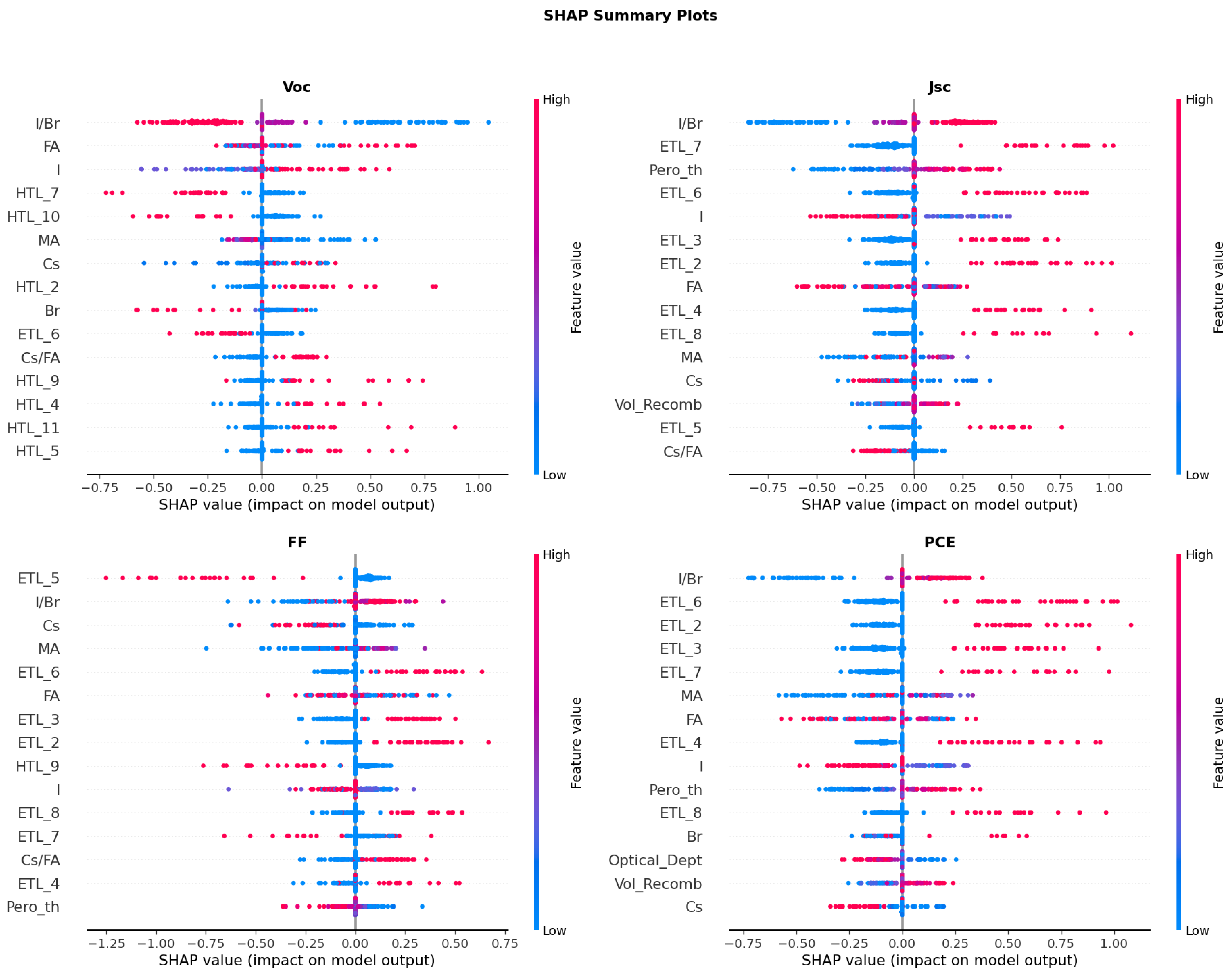
The SHAP analysis in Figure 11 extends these results by clarifying the directionality of feature effects. The I/Br ratio exhibits a negative SHAP effect on $V_{oc}$ and a positive effect on $J_{sc}$, reflecting the halide-mediated $V_{oc}$–$J_{sc}$ trade-off: increasing iodide content narrows the bandgap, lowering the open-circuit voltage while broadening the range of absorbed photon wavelengths and thereby increasing the photocurrent. The thickness feature (Pero_th) shows a positive SHAP effect on $J_{sc}$, in agreement with Beer–Lambert absorption enhancement.

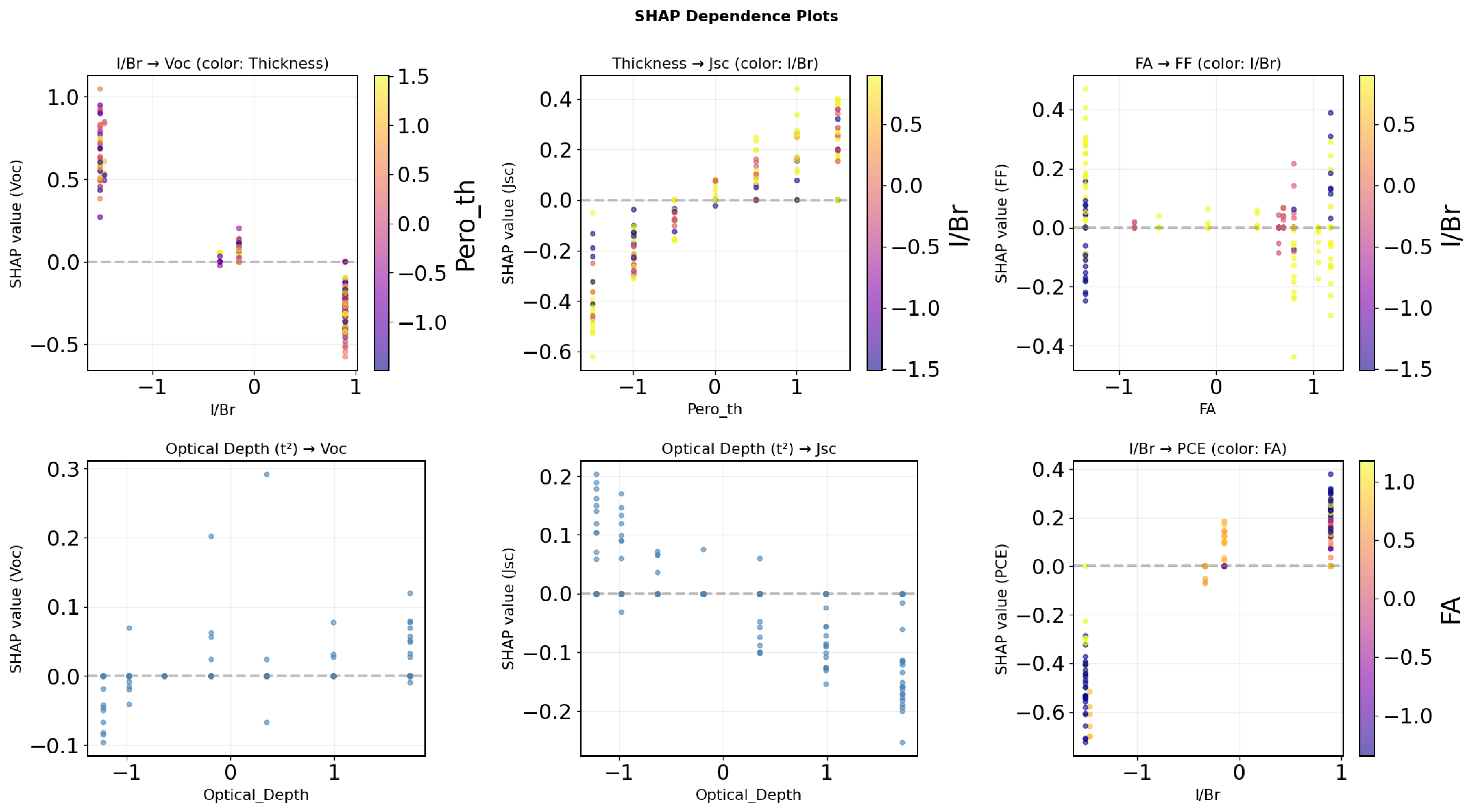
The SHAP dependence plots in Figure 12 reveal non-linear relationships captured by the model, including saturation effects and interaction-driven stratification that are not detectable by linear methods. The convergence of all three interpretability analyses (permutation importance, SHAP beeswarm, and SHAP dependence) on the same physical narrative provides confidence that the model has captured the statistical correlations present in the SCAPS-1D simulation outputs rather than exploiting spurious correlations.

3.9. Hyperparameter Sensitivity

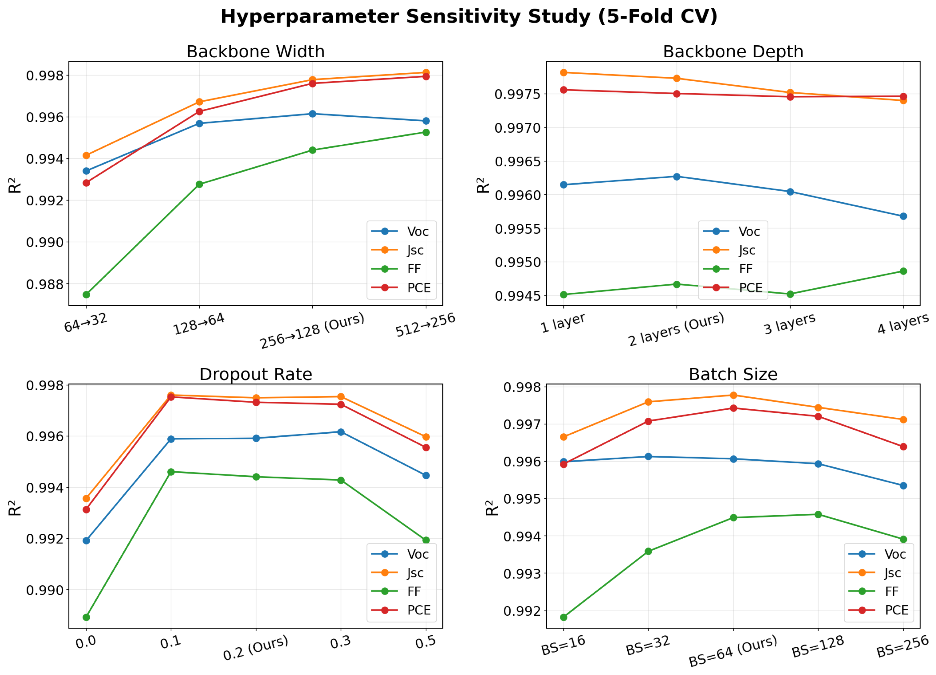
A hyperparameter sensitivity study across four architectural dimensions, as depicted in

Table 15. Hyperparameter sensitivity (5-fold CV $R^2$).

Study	Configuration	${\mathit{V}}_{\mathit{oc}}$${\mathit{R}}^2$	${\mathit{J}}_{\mathit{sc}}$${\mathit{R}}^2$	FF ${\mathit{R}}^2$	PCE ${\mathit{R}}^2$
Width	$64\to 32$	0.993	0.994	0.987	0.993
	$128\to 64$	0.996	0.997	0.993	0.996
	$256\to 128$ (Ours)	0.996	0.998	0.994	0.998
	$512\to 256$	0.996	0.998	0.995	0.998
Depth	1 layer	0.996	0.998	0.995	0.998
	2 layers (Ours)	0.996	0.998	0.995	0.998
	3 layers	0.996	0.998	0.995	0.997
	4 layers	0.996	0.997	0.995	0.997
Dropout	0.0	0.992	0.994	0.989	0.993
	0.1	0.996	0.998	0.995	0.998
	0.2 (Ours)	0.996	0.997	0.994	0.997
	0.3	0.996	0.998	0.994	0.997
	0.5	0.994	0.996	0.992	0.996
Batch Size	16	0.996	0.997	0.992	0.996
	32	0.996	0.998	0.994	0.997
	64 (Ours)	0.996	0.998	0.994	0.997
	128	0.996	0.997	0.995	0.997
	256	0.995	0.997	0.994	0.996

and Figure 13, examines whether the reported results depend on specific hyperparameter choices or reflect a broad basin of good performance. Backbone width was scaled from $64\to 32$ to $512\to 256$. The smallest configuration shows measurable degradation, particularly for FF ($R^2=0.987$). From $128\to 64$ onward, all targets achieve $R^2\ge 0.993$ and gains plateau. The chosen width ($256\to 128$) performs nearly identically to the larger $512\to 256$ with half the parameters.

As for backbone depth, it was varied from 1 to 4 layers. $R^2$ varies by at most 0.001 for any target across this range, which suggests that the 128-dimensional latent representation captures sufficient complexity regardless of the number of transformation stages and that head-level capacity, rather than backbone depth, governs per-target performance.

The dropout rate was swept from $p=0.0$ to $p=0.5$. Disabling dropout entirely produces the worst performance across all targets (FF $R^2=0.989$), confirming that regularization remains necessary even in the multi-task setting. Performance peaks at $p=0.1$–$0.2$ and degrades at $p=0.5$. The chosen value ($p=0.2$) lies near the optimum.

The batch size was varied from 16 to 256. Performance peaks at 64–128, with both smaller and larger sizes showing slight degradation for FF. The total $R^2$ range for FF across the full span is 0.003, making this the mildest of the four sensitivities. Across all four studies, FF is consistently the most sensitive target, which corroborates the finding that FF prediction is inherently the most difficult and benefits the most from the multi-task architecture.

4. Discussion

4.1. Why Multi-Task Learning Stabilizes Prediction

The observed multi-task advantage can be attributed to cross-task gradient regularization. In the single-task FF model, the backbone receives gradients from FF prediction errors alone. When a given data partition underrepresents the feature interactions governing fill factor, the backbone lacks corrective signals. It overfits or underfits, and the result is the catastrophic $R^2$ collapses of Folds 3 and 4 ($R^2=0.321$ and 0.332). The multi-task backbone, on the other hand, receives gradient information from $V_{oc}$, $J_{sc}$, and PCE—all of which share physical origins with FF. These gradients act as implicit regularizers that stabilize the learned representation even when the FF-specific signal is weak.

The single-task FF collapse is not an artifact of poor hyperparameter tuning. The single-task models use an architecture, optimizer, learning rate, and callback configuration identical to those of the corresponding multi-task prediction heads, with the sole difference being the absence of the shared backbone. Fresh EarlyStopping and ReduceLROnPlateau callbacks are instantiated for every training run to prevent state leakage across folds. The same single-task training pipeline achieves $R^2\ge 0.87$ on Voc, Jsc, and PCE, demonstrating that the training procedure is effective. The FF-specific instability arises from the physical complexity of fill factor, which depends on the interplay of series resistance, shunt resistance, recombination, and charge transport. It is this dependence that creates a less smooth loss landscape than the other targets. The shared backbone in the multi-task model stabilizes FF learning by providing gradient information from correlated tasks.

Several lines of evidence substantiate this interpretation. Variance reduction is most pronounced for the target with the most complex underlying physics (FF, 233-fold), where regularization affords the greatest benefit. The reduction in cross-fold standard deviation is orders of magnitude greater than the mean $R^2$ improvement, indicating that the primary gain is stability, not an increased accuracy ceiling. Per-composition and per-ETL analyses (Table 12 and Table 13) reveal minimal subgroup-level gains (mean $|\Delta R^2|$ of 0.006 and 0.002, respectively), which is consistent with fold-level regularization rather than subgroup-specific learning. Moreover, per-fold consistency data (Table 8) show that single-task consistency deteriorates in precisely the folds where FF collapses—Fold 3 (consistency MAE = 2.424, FF $R^2=0.321$) and Fold 4 (2.235, 0.332), a correlation that establishes a direct link between per-target failure and inter-parameter inconsistency. The hyperparameter sensitivity study (Table 15) further confirms that the advantage persists across a broad range of backbone widths, depths, dropout rates, and batch sizes, ruling out an explanation based on fragile architectural tuning.

It should be noted that this interpretation does not assert that the shared backbone has learned specific latent physical variables. Such an assertion would require probing internal representations using linear probes, which we designate for future work. What we do claim is that the multi-task architecture affords a strong empirical defense against catastrophic target-specific failure. As shown in Section 4.3, post hoc algebraic correction of single-task outputs eliminates consistency error by construction but cannot rescue the degraded PCE accuracy that results from compounding the errors of three independently unstable predictors.

4.2. The CatBoost Question: Consistency Without Shared Representations

CatBoost achieves a consistency MAE of $0.255\pm 0.008$ across four independent models, matching the MH-NN’s $0.264\pm 0.024$. This indicates that on a smooth, deterministic simulation manifold where individual predictions are accurate ($R^2\ge 0.962$), physical consistency is arithmetically maintained. When each parameter is predicted within approximately 1–2% error, the product $V_{oc}\times J_{sc}\times \mathrm{FF}/100$ will closely approximate the directly predicted PCE regardless of whether the models share representations.

Three factors distinguish the MH-NN in practice. First, CatBoost’s FF $R^2$ (0.962) is lower than the MH-NN’s (0.994), a difference of 0.032 that is likely to widen on experimental data subject to measurement noise and unmodeled physical effects. Second, CatBoost’s low variance (standard deviation $\le 0.002$) reflects the inherent stability of gradient-boosted tree ensembles, which are resistant to the fold-dependent training instabilities observed in neural networks. As a consequence, the most informative comparison is between multi-task and single-task neural networks, i.e., the same model class with and without multi-task learning, where the consistency improvement is substantial (0.264 vs. 1.871). Third, neural networks afford advantages that tree-based methods do not, including differentiability for gradient-based optimization, scalability to larger feature spaces, and integration with physics-constrained loss functions. These properties make the multi-task stabilization of neural networks a practical advancement even when tree-based alternatives are available.

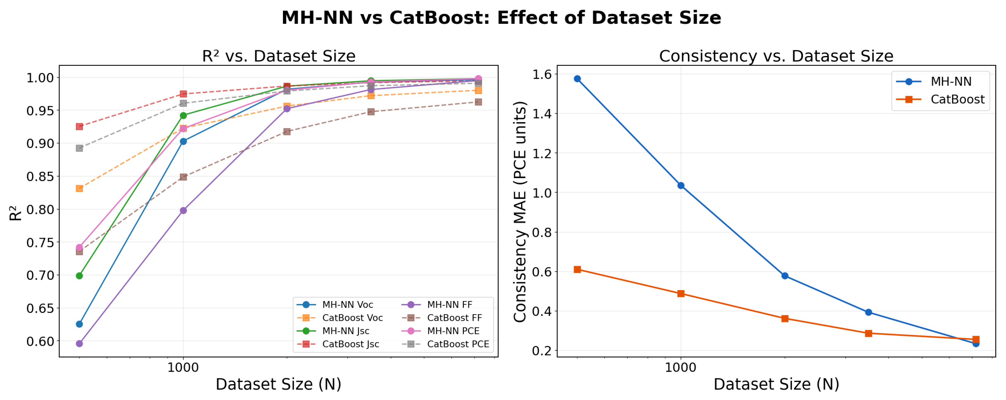
A dataset-size scaling experiment further clarifies the MH-NN vs. CatBoost trade-off. At $N=500$, CatBoost dominates across all four targets (e.g., FF $R^2=0.736$ vs. 0.596 for MH-NN) and achieves substantially better consistency (MAE $=0.610$ vs. 1.576). The MH-NN overtakes CatBoost on per-target $R^2$ between $N=2000$ and $N=3500$, with the crossover for consistency occurring at the full dataset size ($N=7176$). This pattern is consistent with the general finding that gradient-boosted trees have stronger built-in regularization at small sample sizes, while neural networks require sufficient data for their shared-representation advantage to manifest. For the SCAPS-1D simulation pipeline, where generating thousands of samples is computationally inexpensive, the MH-NN is the appropriate choice; for small experimental datasets, CatBoost would likely be preferable (Figure 14).

4.3. Post-Processing Algebraic Correction

A natural question is whether a simple algebraic correction, replacing the single-task PCE prediction with $V_{oc,\mathrm{pred}}\times J_{sc,\mathrm{pred}}\times {\mathrm{FF}}_{\mathrm{pred}}/100$, would eliminate the need for multi-task learning to achieve consistency. We implemented this baseline and evaluated it across all five folds, as shown in

Table 16. Post-processing algebraic correction baseline. The corrected single-task model replaces the independently predicted PCE with $V_{oc,\mathrm{pred}}\times J_{sc,\mathrm{pred}}\times {\mathrm{FF}}_{\mathrm{pred}}/100$. Consistency error is eliminated by construction, but PCE $R^2$ degrades due to compounded prediction errors from the three upstream single-task models.

Fold	ST PCE ${\mathit{R}}^2$	STcorr PCE ${\mathit{R}}^2$	MT PCE ${\mathit{R}}^2$	ST Cons.	STcorr Cons.	MT Cons.
1	0.927	0.822	0.997	2.264	0.000	0.209
2	0.905	0.900	0.998	1.291	0.000	0.239
3	0.945	0.942	0.998	0.872	0.000	0.246
4	0.900	0.800	0.997	2.090	0.000	0.242
5	0.884	0.894	0.998	1.325	0.000	0.243
Mean ± std	$0.912\pm 0.022$	$0.872\pm 0.053$	$0.997\pm 0.001$	$1.568\pm 0.518$	$0.000$	$0.236\pm 0.014$

.

By construction, the corrected single-task model achieves zero consistency error: the predicted PCE is defined as the product of the other three predictions. However, the corrected PCE $R^2$ degrades substantially compared to the multi-task model. Across folds, the corrected single-task PCE $R^2$ averages $0.872\pm 0.053$, compared to $0.997\pm 0.001$ for the multi-task model. The degradation is most severe in the folds where FF collapses: in Fold 1 (FF $R^2=0.341$), the corrected PCE $R^2$ drops to $0.822$, while the multi-task PCE $R^2$ remains at $0.997$.

This result demonstrates that consistency and accuracy are not interchangeable objectives. Post-processing can enforce algebraic agreement, but it cannot compensate for the compounded errors of three independently trained and potentially unstable predictors. Multi-task learning achieves both objectives simultaneously by stabilizing the shared representation from which all four predictions originate.

4.4. Architectural Robustness and Hyperparameter Stability

The hyperparameter sensitivity study (Section 3.9) confirms that the reported results are not the product of fragile tuning. Across 18 configurations spanning four dimensions, all but one achieve $R^2>0.993$ on every target. Degradation occurs only at the extremes: the smallest backbone ($64\to 32$) and zero dropout, both of which lie outside the reasonable design space for a dataset of this size. The chosen configuration occupies a broad plateau where performance is essentially invariant to perturbation.

The loss weighting ablation (Section 3.2) provides a complementary perspective. While $R^2$ is invariant to weight choice, consistency MAE responds monotonically to FF overweighting (from 0.222 at uniform to 0.291 at FF × 5). This dissociation between $R^2$ stability and consistency sensitivity suggests that consistency MAE is a more discriminating metric than $R^2$ in the high-accuracy regime, a finding with methodological implications for future multi-output prediction studies.

The Kendall et al. homoscedastic uncertainty framework [20] was also evaluated as an alternative to manual weight selection.

Table 17. Kendall learned-weight vs. manual $[1,1,2,1]$ configuration (5-fold CV). Learned weights are reported as effective precision ($1/{\sigma }^2$) and normalized relative to $J_{sc}$.

Target	Kendall ${\mathit{R}}^2$	Manual ${\mathit{R}}^2$	$\mathbf{\Delta }{\mathit{R}}^2$	Learned $1/{\mathit{\sigma }}^2$	Norm.
$V_{oc}$	$0.996\pm 0.001$	$0.996\pm 0.001$	$+0.000$	$304.6\pm 39.5$	1.25
$J_{sc}$	$0.998\pm 0.001$	$0.998\pm 0.001$	$+0.000$	$244.4\pm 42.7$	1.00
FF	$0.995\pm 0.001$	$0.994\pm 0.001$	$+0.001$	$109.2\pm 14.7$	0.45
PCE	$0.998\pm 0.000$	$0.997\pm 0.001$	$+0.001$	$208.1\pm 34.0$	0.85
Cons. MAE	$0.201\pm 0.022$	$0.264\pm 0.024$	$-0.063$	—	—

shows that the learned-weight model achieves $R^2$ values within $\pm 0.001$ of the manual $[1,1,2,1]$ configuration on all targets and slightly better consistency (MAE $=0.201$ vs. $0.264$). The learned effective weights (precision $1/{\sigma }^2$: Voc: 304.6, Jsc: 244.4, FF: 109.2, PCE: 208.1; normalized relative to $J_{sc}$: 1.25, 1.00, 0.45, 0.85) reveal that the model assigns FF the lowest precision (highest uncertainty), consistent with FF being the most physically complex and hardest-to-predict target. This data-driven validation confirms that the manual weight selection is near-optimal for the present dataset and provides a principled framework for automatic weight tuning on future datasets where task uncertainties may differ.

4.5. Feature Construction and Domain Knowledge

The feature ablation study in Section 3.1 and permutation importance analysis in Section 3.8 together yield a nuanced view of domain knowledge injection. The six physics-guided features improve consistency by 8.3% (0.254 vs. 0.277) but do not improve $R^2$, which indicates that the multi-task network can discover task-relevant interactions from raw inputs, but benefits from precomputed representations for inter-parameter coherence.

Permutation importance reveals a physically interpretable feature hierarchy (Table 14): the I/Br ratio dominates $V_{oc}$ (0.631) via bandgap control, the FA fraction dominates $J_{sc}$ (0.557) via absorption, and ETL categories dominate FF and PCE via charge extraction. The engineered Cs/FA ratio (importance 0.235–0.251) contributes across all targets, confirming its role in capturing tolerance factor physics. The fact that the model independently reproduces the $V_{oc}$–$J_{sc}$ trade-off (opposing SHAP signs for I/Br) and the thickness–$J_{sc}$ Beer–Lambert relationship provides confidence in its suitability for virtual screening within the simulator’s domain.

4.6. Practical Implications for Virtual Screening

The results suggest four practical applications. First, the consistency metric provides a natural filter for screening pipelines: predictions exceeding the 2 PCE-unit threshold can be flagged and rejected, eliminating the 36.5% of single-task predictions that are physically implausible. Second, simultaneous prediction of four coupled parameters enables multi-objective optimization, for instance, identifying device configurations that maximize $V_{oc}$ while maintaining FF above a minimum threshold. Third, the single-forward-pass architecture produces four predictions in one inference call, reducing computational cost relative to four independent models. Fourth, the SHAP-identified feature hierarchies provide directly interpretable design rules: modify halide composition to increase $V_{oc}$, increase FA fraction, optimize ETL choice to increase $J_{sc}$, and focus on ETL engineering to improve FF. These rules are derived from the model’s learned representations and validated against established photovoltaic physics.

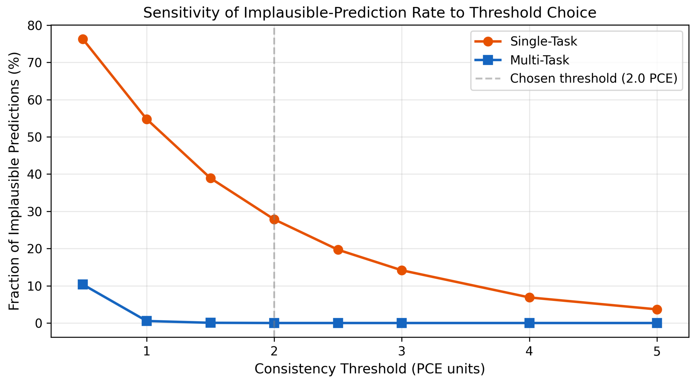
A threshold sensitivity analysis confirms that the multi-task consistency advantage is robust to the choice of threshold (Figure 15). Across thresholds from 0.5 to 5.0 PCE units, the fraction of implausible single-task predictions decreases monotonically from 76.3% to 3.7%, while the multi-task fraction drops to 0.54% at 1.0 PCE units (39 samples), 0.06% at 1.5 PCE units (4 samples), and zero above 2.0 PCE units. The ratio of single-task to multi-task implausible predictions exceeds 100× at a 1.0 PCE threshold and is infinite above 2.0 PCE. The chosen 2 PCE-unit threshold is therefore conservative; the conclusion holds at any reasonable threshold.

4.7. Robustness to Measurement Noise

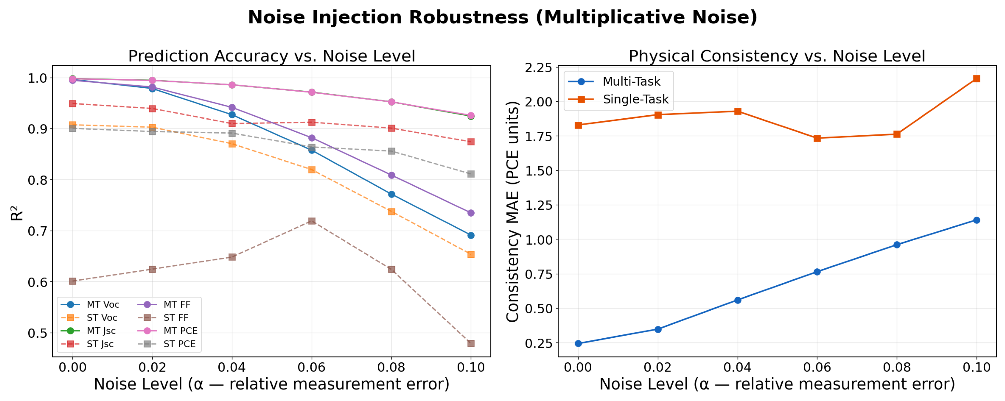
To assess whether the multi-task advantage transfers to noisy conditions representative of experimental data, multiplicative Gaussian noise was injected into all four targets at levels of $\alpha \in \{0,0.02,0.04,0.06,0.08,0.10\}$, where $\alpha$ denotes the relative measurement error (e.g., $\alpha =0.05$ corresponds to 5% instrument uncertainty). Both multi-task and single-task models were retrained under 5-fold cross-validation at each noise level.

The multi-task model degrades monotonically and gracefully: FF $R^2$ decreases from $0.994$ ($\alpha =0$) to $0.735$ ($\alpha =0.10$), and consistency MAE increases from $0.244$ to $1.140$. The single-task model degrades more rapidly and erratically: FF $R^2$ drops from $0.601$ to $0.479$, while consistency MAE increases from $1.905$ to $2.165$. At $\alpha =0.10$, a stress-test level exceeding typical experimental uncertainty, the multi-task model under heavy noise achieves better consistency ($1.140$) than the single-task model on perfectly clean data ($1.905$). These results suggest that the multi-task advantage is not an artifact of noise-free simulation and is likely to persist on experimental data (Figure 16).

4.8. Limitations

We state the following limitations directly. SCAPS-1D is a one-dimensional drift-diffusion solver that cannot capture grain boundary passivation, spatial inhomogeneity, or interfacial roughness. Ion migration and J–V hysteresis are not modeled. The noise-free simulation manifold inflates absolute $R^2$ values; the transferable finding is the relative advantage of multi-task over single-task baselines. Material parameters are predefined from literature values and may not span the full range of experimental variability. The dataset is limited to 12 perovskite compositions, 8 ETL types, and a predominantly n-i-p architecture. A leave-one-composition-out (LOCO) experiment, shown in

Table 18. Leave-one-composition-out (LOCO) results. Multi-task $R^2$ on held-out compositions not seen during training. Negative $R^2$ indicates predictions worse than the target mean. Single-task results are similarly catastrophic.

Held-Out Composition	${\mathit{N}}_{\mathbf{test}}$	${\mathit{V}}_{\mathit{oc}}$${\mathit{R}}^2$	${\mathit{J}}_{\mathit{sc}}$${\mathit{R}}^2$	FF ${\mathit{R}}^2$	PCE ${\mathit{R}}^2$
CsPbI3	1008	$-2.354$	$-7.595$	$+0.295$	$-0.862$
MAPbI3	1001	$-0.689$	$-2.226$	$-0.636$	$-2.198$
FAPbI3	903	$-1.322$	$-1.476$	$-2.437$	$-0.528$
Cs0.15FA0.85PbI3	974	$-2.703$	$-2.667$	$-0.985$	$-4.076$

, confirms that the model is designed for interpolation, not extrapolation. When an entire composition is held out during training (e.g., CsPbI₃, MAPbI₃, FAPbI₃, or Cs_0.15FA_0.85PbI₃), the model produces catastrophically poor predictions on the unseen chemistry, with $R^2$ values ranging from $-7.6$ to $+0.3$ across targets and compositions. This is expected: the compositional features (Cs, MA, FA fractions) take values during testing that were absent during training, and the model has no basis for extrapolation. Compositional generalization to genuinely novel chemistries would require composition-aware encodings, meta-learning, or transfer learning approaches, which we designate for future work. Fixed loss weighting is employed rather than learned weighting [20]; the sensitivity study in Section 3.2 mitigates but does not eliminate this concern. Physical consistency in the proposed model is emergent, not enforced–the model is not constrained to satisfy Equation (1) exactly. No uncertainty quantification is provided for individual predictions. Finally, the CatBoost consistency equivalence suggests that the multi-task consistency advantage may be specific to scenarios where individual accuracy is unreliable, which is precisely the scenario expected on experimental data.

The 5-fold cross-validation design yields $n=5$ paired observations per statistical test. While effect sizes are large (Cohen’s $d=1.33$–$8.93$) and paired t-tests are significant ($p<0.05$ for all targets), the Wilcoxon signed-rank test has a minimum achievable p-value of $0.0625$ with $n=5$, which precludes significance at the conventional $\alpha =0.05$ level. We therefore emphasize effect sizes and practical significance (20/20 fold dominance) over p-values in our inferential claims.

5. Conclusions

A multi-head neural network for the simultaneous prediction of $V_{oc}$, $J_{sc}$, FF, and PCE in perovskite solar cells was validated on 7176 SCAPS-1D simulated device configurations spanning 12 compositions. The following four principal findings emerged. First, multi-task learning rescued the FF prediction from catastrophic instability ($R^2=0.617\pm 0.254$, single-task) to stable accuracy ($R^2=0.994\pm 0.001$), a 233-fold reduction in cross-fold standard deviation. The multi-task model achieved a higher $R^2$ than the single-task baseline in all 20-fold target comparisons. Second, the physical consistency metric introduced in this work revealed that 36.5% of single-task predictions are physically implausible, exceeding a 2 PCE-unit mismatch threshold, compared to 0.014% for multi-task predictions. This failure mode is not detectable by per-target $R^2$ alone. The metric is applicable to any multi-output prediction task in which the targets are related by a known physical equation. Third, the MH-NN achieved the highest $R^2$ among all evaluated models (≥0.994 on every target) while producing four predictions in a single forward pass. CatBoost achieved comparable consistency on this smooth simulation manifold ($0.255\pm 0.008$ vs. $0.264\pm 0.024$), which confirms that high individual accuracy suffices for consistency on clean data and motivates experimental validation where individual accuracy is less reliable. Fourth, SHAP analysis and permutation importance confirmed that the model captures the statistical correlations present in the SCAPS-1D simulation outputs, including halide-mediated bandgap control, the Beer–Lambert absorption relationship, and ETL-dominated efficiency determination.

Additional experiments strengthened these conclusions. A post-processing algebraic correction baseline demonstrated that enforcing consistency through ${\mathrm{PCE}}_{\mathrm{corrected}}=V_{oc,\mathrm{pred}}\times J_{sc,\mathrm{pred}}\times {\mathrm{FF}}_{\mathrm{pred}}/100$ eliminates consistency error by construction but degrades PCE $R^2$ to $0.871\pm 0.052$, compared to $0.997\pm 0.001$ for the multi-task model, because the correction compounds the errors of three independently unstable predictors. Noise injection experiments with multiplicative Gaussian noise ($\alpha =0$–$0.10$ relative measurement error) confirmed that the multi-task advantage persists under realistic experimental uncertainty, with the multi-task model under 10% noise maintaining better consistency than the single-task model on clean data. Dataset-size scaling experiments revealed that CatBoost outperforms the MH-NN at $N\le 1000$ but that the MH-NN overtakes CatBoost on per-target accuracy for $N\ge 3500$, with consistency converging at the full dataset size. A Kendall learned-weight framework validated the manual selection of loss weights and identified FF as the target with the highest aleatoric uncertainty. These results collectively demonstrate that the multi-task advantage is robust, data-regime-dependent, and not reducible to algebraic enforcement.

An avenue for further research would be to transfer the model to experimental PSC datasets via fine-tuning or domain adaptation, testing whether the multi-task robustness advantage persists on noisy data. Other directions include embedding the PCE equation as a physics-constrained auxiliary loss to convert emergent consistency into enforced consistency, incorporating calibrated uncertainty quantification via conformal prediction or deep ensembles, and probing the latent space via linear probes to determine whether backbone activations correlate with known physical quantities.

References

1. Li, G.; Zhang, Z.; Agyei-Tuffour, B.; Wu, L.; Gries, T.; Prashanthan, K.; Frohloff, L.; Musiienko, A.; Li, J.; Zhu, R.; et al. Stabilizing high-efficiency perovskite solar cells via strategic interfacial contact engineering. Nat. Photonics 2026, 20, 55–62, Correction in Nat. Photonics 2026, 20, 241. https://doi.org/10.1038/s41566-025-01791-1. [Google Scholar] [CrossRef] [Scilit] [PubMed]
2. Al Atem, M.; Dridi Rezgui, B.; Touhami, I.; Bouaïcha, M. Numerical simulation and optimization of high-performance lead-based FAMACsPb(IBr)3 perovskite solar cells using SCAPS 1D. Results Eng. 2026, 29, 108555. [Google Scholar] [CrossRef] [Scilit]
3. Rabhi, S.; Benzouid, H.; Slami, A.; Dadda, K. Modeling and numerical simulation of a CH3NH3SnI3 perovskite solar cell using the SCAPS1-D simulator. Eng. Proc. 2023, 56, 97. [Google Scholar] [CrossRef] [Scilit]
4. Al Atem, M.; Makableh, Y. Towards Sustainable Perovskite Solar Cells: Lead-Free High Efficiency Designs with Tin and Germanium. Eng 2025, 6, 38. [Google Scholar] [CrossRef] [Scilit]
5. Al Atem, M.; Makableh, Y.; Arnaout, M. Analytical Solutions for Current–Voltage Properties of PSCs and Equivalent Circuit Approximation. Eng 2025, 6, 62. [Google Scholar] [CrossRef] [Scilit]
6. Li, Z.; Huang, C.; Chao, L.; Chen, Y.; Huang, W.; Chen, G. Perovskite solar cells empowered by machine learning. J. Energy Chem. 2025, 109, 403–437. [Google Scholar] [CrossRef] [Scilit]
7. Chen, Z.; Pan, S.; Wang, J.; Min, Y.; Chen, Y.; Xue, Q. Machine learning will revolutionize perovskite solar cells. Innovation 2024, 5, 100602. [Google Scholar] [CrossRef] [Scilit] [PubMed]
8. Mao, L.; Xiang, C. A comprehensive review of machine learning applications in perovskite solar cells: Materials discovery, device performance, process optimization and systems integration. Mater. Today Energy 2025, 47, 101742. [Google Scholar] [CrossRef] [Scilit]
9. Novoselov, I.; Gvozdev, A.; Smirnov, A.; Zhidkov, I. Dataset of SCAPS-1D simulated halide perovskite solar cells with SHAP and machine learning-based PCE optimization. Data Brief 2025, 60, 111653. [Google Scholar] [CrossRef] [Scilit] [PubMed]
10. Reza, M.; Ghosh, A.; Shimul, A.; Nabil, S.; Akter, M.; Chaudhry, A.; Sobuj, D.; Kumar, Y.; Biswas, S.; Alam, K.; et al. Simulation and machine learning driven optimization of Rb2SnBr6-based lead-free perovskite solar cells using diverse ETLs for enhanced photovoltaic performance. Mater. Adv. 2025, 6, 9602–9626. [Google Scholar] [CrossRef] [Scilit]
11. Li, W.; Hu, J.; Chen, Z.; Jiang, H.; Wu, J.; Meng, X.; Fang, X.; Lin, J.; Ma, X.; Yang, T.; et al. Performance prediction and optimization of perovskite solar cells based on the Bayesian approach. Sol. Energy 2023, 262, 111853. [Google Scholar] [CrossRef] [Scilit]
12. Saidani, O.; Yousfi, A.; Belhadad, Y.; Zouache, R.; Brahimi, A.; Sahoo, G. Predictive modeling of Rb2ScCuCl6-based perovskite solar cells performance using neural networks-guided optimization and SHAP-based interpretability. J. Phys. Chem. Solids 2026, 208, 113084. [Google Scholar] [CrossRef] [Scilit]
13. Caruana, R. Multitask learning. Mach. Learn. 1997, 28, 41–75. [Google Scholar] [CrossRef] [Scilit]
14. Li, W.; Zhang, H.; van Vlijmen, B.; Dechent, P.; Sauer, D. Forecasting battery capacity and power degradation with multi-task learning. Energy Storage Mater. 2022, 53, 453–466. [Google Scholar] [CrossRef] [Scilit]
15. Jacobsson, T.; Hultqvist, A.; García-Fernández, A.; Anand, A.; Al-Ashouri, A.; Hagfeldt, A.; Crovetto, A.; Abate, A.; Ricciardulli, A.G.; Vijayan, A.; et al. An open-access database and analysis tool for perovskite solar cells based on the FAIR data principles. Nat. Energy 2022, 7, 107–115. [Google Scholar] [CrossRef] [Scilit]
16. Burgelman, M.; Nollet, P.; Degrave, S. Modelling polycrystalline semiconductor solar cells. Thin Solid Film. 2000, 361–362, 527–532. [Google Scholar] [CrossRef] [Scilit]
17. Raissi, M.; Perdikaris, P.; Karniadakis, G. Physics-informed neural networks: A deep learning framework for solving forward and inverse problems involving nonlinear partial differential equations. J. Comput. Phys. 2019, 378, 686–707. [Google Scholar] [CrossRef] [Scilit]
18. Ioffe, S.; Szegedy, C. Batch normalization: Accelerating deep network training by reducing internal covariate shift. In Proceedings of the 32nd International Conference on Machine Learning (ICML), Lille, France, 6–11 July 2015; pp. 448–456. [Google Scholar]
19. Srivastava, N.; Hinton, G.; Krizhevsky, A.; Sutskever, I.; Salakhutdinov, R. Dropout: A simple way to prevent neural networks from overfitting. J. Mach. Learn. Res. 2014, 15, 1929–1958. [Google Scholar]
20. Cipolla, R.; Gal, Y.; Kendall, A. Multi-task learning using uncertainty to weigh losses for scene geometry and semantics. In 2018 IEEE/CVF Conference on Computer Vision and Pattern Recognition (CVPR); IEEE: Piscataway, NJ, USA, 2018; pp. 7482–7491. [Google Scholar] [CrossRef] [Scilit]
21. Loshchilov, I.; Hutter, F. Decoupled weight decay regularization. In Proceedings of the International Conference on Learning Representations (ICLR), New Orleans, LA, USA, 6–9 May 2019. [Google Scholar]
22. Chen, T.; Guestrin, C. XGBoost: A scalable tree boosting system. In Proceedings of the 22nd ACM SIGKDD International Conference on Knowledge Discovery and Data Mining; Association for Computing Machinery: New York, NY, USA, 2016; pp. 785–794. [Google Scholar] [CrossRef] [Scilit]
23. Prokhorenkova, L.; Gusev, G.; Vorobev, A.; Dorogush, A.; Gurevich, A. CatBoost: Unbiased boosting with categorical features. In Proceedings of the Advances in Neural Information Processing Systems (NeurIPS); Association for Computing Machinery: New York, NY, USA, 2018; pp. 6638–6648. [Google Scholar]
Figure 1. Multi-head neural network architecture. A shared backbone (dashed box) compresses 29 input features into a 128-dimensional device-state representation. Four task-specific prediction heads, with depths calibrated to target complexity, branch from this shared representation to produce scalar estimates of V o c , J s c , FF, and PCE. Total model parameters: ≈83,000.
Inventions 11 00059 g001
Figure 2. Experimental design overview.
Inventions 11 00059 g002
Figure 3. Feature engineering ablation. Horizontal bars show R 2 for each target under six feature configurations. All configurations achieve R 2 > 0.994 , demonstrating that the multi-task architecture is the primary driver of prediction accuracy, with physics-guided features providing marginal gains in inter-parameter consistency.
Inventions 11 00059 g003
Figure 4. Loss weighting sensitivity heatmap. R 2 per target across six weight configurations. All cells exceed 0.994, confirming that prediction accuracy is invariant to the choice of loss weights within the tested range. On the vertical axis, “↓” denotes a down-weighted task.
Inventions 11 00059 g004
Figure 5. Physical consistency error by loss weighting. Uniform weighting [ 1 , 1 , 1 , 1 ] achieves the lowest consistency MAE (0.222), while increasing FF emphasis progressively degrades consistency. Error bars indicate cross-fold standard deviation. Error bars indicate cross-fold standard deviation ( n = 5 ).
Inventions 11 00059 g005
Figure 6. Per-fold R 2 for single-task (red) and multi-task (blue) models across all four targets. Single-task FF R 2 ranges from 0.321 to 0.907, while multi-task maintains R 2 0.993 in all folds. The 233× reduction in cross-fold standard deviation demonstrates qualitative transformation from unreliable to stable prediction.
Inventions 11 00059 g006
Figure 7. Distribution of signed consistency errors. Multi-task predictions (blue) are tightly concentrated near zero, while single-task predictions (red) exhibit heavy tails. Dashed lines indicate the ±2 PCE-unit implausibility threshold. 36.5% of single-task predictions exceed this threshold versus 0.014% for multi-task.
Inventions 11 00059 g007
Figure 8. Model comparison across all four targets. The MH-NN achieves the highest R 2 on every target with the tightest cross-fold variability. CatBoost is the strongest tree-based competitor, while XGBoost shows the weakest performance, particularly on FF. Error bars indicate cross-fold standard deviation ( n = 5 ).
Inventions 11 00059 g008
Figure 9. Per-composition Δ R 2 (MT − ST) heatmap across 12 perovskite compositions and four targets. Most differences are negligible ( | Δ R 2 | < 0.01 ), confirming that the multi-task advantage arises from fold-level stabilization rather than composition-specific accuracy gains.
Inventions 11 00059 g009
Figure 10. Permutation importance (50 repetitions, 95% CI) for the top features across all four targets. The I/Br ratio dominates V o c prediction (0.631), FA fraction dominates J s c (0.557) and PCE (0.523), and multiple ETL categories appear as critical features for J s c , FF, and PCE.
Inventions 11 00059 g010
Figure 11. SHAP beeswarm summary for all four targets. Red indicates high feature values, blue indicates low. The analysis confirms the halide-mediated V o c J s c trade-off (I/Br shows opposing signs across targets), the thickness– J s c Beer–Lambert relationship, and ETL-dominated FF and PCE control.
Inventions 11 00059 g011
Figure 12. SHAP dependence plots for selected feature–target pairs. Non-linear relationships and interaction effects are visible, including saturation behavior in the I/Br– V o c relationship and FA-dependent stratification in the I/Br–PCE relationship.
Inventions 11 00059 g012
Figure 13. Hyperparameter sensitivity across four studies: backbone width, backbone depth, dropout rate, and batch size. R 2 for all four targets remains above 0.99 across most configurations, with FF consistently the most sensitive target. The chosen configuration (marked) lies in the plateau region for all studies.
Inventions 11 00059 g013
Figure 14. Dataset-size scaling comparison between MH-NN and CatBoost. Left: per-target R 2 as a function of training set size. Right: consistency MAE as a function of training set size. CatBoost dominates at N 1000 ; MH-NN overtakes on R 2 at N 3500 with consistency converging at the full dataset.
Inventions 11 00059 g014
Figure 15. Sensitivity of the implausible-prediction rate to the consistency threshold. The multi-task model reaches zero violations above 2.0 PCE units, while the single-task model retains substantial violation rates across all thresholds.
Inventions 11 00059 g015
Figure 16. Noise injection robustness study with multiplicative Gaussian noise ( α = 0 0.10 relative measurement error). (Left) per-target R 2 degradation. The MT J s c (green) and MT PCE (pink) curves nearly coincide and appear as a single curve. (Right) consistency MAE degradation. The multi-task model degrades monotonically and maintains better consistency at α = 0.10 than the single-task model on clean data.
Inventions 11 00059 g016