Conquering the Urban Firefighting Challenge: A Deep Q-Network Approach for Autonomous UAV Navigation

Abstract

Firefighters must locate victims reliably to carry out rescue operations within burning structures during urban firefighting events. Low visibility, reduced oxygen levels, weakened structural rigidity, and dense smoke make it difficult to locate victims. In addition to these challenges, victims may be unconscious and unable to report their locations to firefighters. This research work explores the Double Deep Q-Network (Double DQN), Dueling Deep Q-Network (Dueling DQN), and Dueling Double Deep Q-Network (D3QN) agents for an unmanned aerial vehicle (UAV) to navigate around a structure and locate trapped victims within it. The UAV’s position, Light Detection and Ranging (LiDAR), and infrared camera data are utilized as inputs for the Deep Q-Networks. The PER is used to store transitions and sample them according to priority for training. Python’s Pygame library is used in this research to create a simulated environment in which infrared camera and LiDAR data are simulated. The performance of the UAV agent is evaluated using cumulative maximum reward, reward distribution histogram, Temporal Difference (TD) error over time, and number of successful episodes. Among the three DQN UAV agents, the Dueling DQN and Double DQN have potential for real-world applications in firefighting.

1. Introduction

Urban fire events are widespread across the United States. According to the U.S. Fire Administration, urban fire events are categorized into three types: one- and two-family residential building fires, multifamily residential building fires, and non-residential building fires. In 2023, 1,389,000 fire incidents occurred, according to the U.S. Fire Administration and the Federal Emergency Management Agency (FEMA) [1]. According to [1], these fires resulted in 3670 deaths and 13,350 injuries. The number of fires in residential buildings in the United States was 344,600 in 2023 [2]. Fire events in residential buildings caused 2890 deaths and 10,400 injuries in 2023. Non-residential building fire events in the United States occurred at a rate of 110,000 in 2023, resulting in 130 deaths and 1200 injuries [3].

There are two modes of firefighting: offensive and defensive firefighting [4,5]. During the offensive mode of firefighting, firefighters look for victims trapped inside the burning structure and try to rescue them. Then they move into the defensive mode of firefighting. In defensive firefighting, firefighters aim to protect neighboring properties from the fire and prevent its spread. Firefighters adopt a defensive approach only when they are confident that no individuals are trapped within the burning building and that the structure’s integrity has not been jeopardized. The offensive mode is the riskiest for firefighters among these two modes. Firefighters must enter the burning structure to conduct search-and-rescue operations. To search for victims, firefighters listen to the screams of the trapped people. This method may not always provide firefighters with the exact location of the victims. In some scenarios, the victim may not be conscious. They may become unconscious from inhaling smoke and fire-related gases. Many firefighters are injured, and some even lose their lives, during this type of firefighting. Reinforcement learning, when applied to controlling an Unmanned Aerial Vehicle (UAV) for navigation around a structure, can aid firefighters in locating victims trapped inside a burning structure during firefighting operations.

With various applications of machine learning [6,7] in diverse aspects [8] of today’s world, robotics in combination with machine learning has led to more intelligent planning of rescue operations in firefighting [9,10]. To implement scream detection, support vector machine (SVM) and long short-term memory (LSTM) techniques have been investigated [11]. To predict the temperature of burning environments, the Autonomous Embedded System Vehicle (AESV) has been utilized. Researchers have studied the application of both autoregressive integrated moving average (ARIMA) and random forest regressor (RFR) models [12]. It is possible to use unmanned aerial vehicles for intelligent firefighting in addition to unmanned ground vehicles. Quenzel et al. [13] introduced an autonomous Unmanned Aerial Vehicle (UAV)–Unmanned Ground Vehicle (UGV) team capable of fire suppression. Their method used thermal cameras for fire detection and LiDAR for accurate flame localization. During the Grand Challenge, their UGV delivered the maximum water to the fire. Brotee et al. [14] proposed a new path-planning approach for the UAV–UGV coalition in obstructed environments. Their approach divided targets into circular zones based on range and density and used Multi-agent Proximal Policy Optimization (MAPPO) and Multi-agent Deep Deterministic Policy Gradient (MADDPG) to complete the navigation task. Shrestha et al. [15] utilized a NeuroEvolution of Augmenting Topologies (NEAT)-based approach for the autonomous navigation of Unmanned Ground Vehicles (UGVs). NEAT is beneficial in unpredictable and hazardous firefighting environments because it enables neural networks to evolve and adapt. In their research, Recurrent Neural Networks (RNNs) and Feedforward Neural Networks (FNNs) were used to train the rover agent in simulation. The FNN model performed better than the RNN model in terms of the number of successful rover agents. In [16], the researchers used NEAT with a detailed reward and penalty system for the navigation task. They analyzed the UGV’s movement using heatmaps. Transfer learning was applied using pre-trained population information from a previous single-room scenario (trained for 200 generations) to evaluate its impact on results. The transfer learning-based approach outperformed the standard simulations in both the three-room and four-room scenarios. UAVs can support human firefighters in fighting wildfires [17]. Seraj et al. [17] designed an algorithm to enhance teamwork between humans and UAVs during firefighting operations. By using a distributed coverage strategy, the authors successfully identified fire-affected areas while prioritizing the safety of human firefighters. They determined the required number of UAVs based on the analysis of simulation results.

One possible use of UAVs is to control and monitor wildfires, thereby reducing the danger firefighters face. Pena et al. [18] developed a UAV for combating intensive wildfires. This UAV is equipped with features that enable it to operate effectively at night and deliver a substantial amount of water (up to 600 L) for firefighting. In a research paper, Viseras et al. [19] suggested a cooperative reinforcement learning framework that employs multiple UAVs for wildfire monitoring. The authors evaluated the scalability of their value decomposition networks (VDN) and multiple single-trained Q-learning agents (MSTA) reinforcement learning algorithms for up to nine UAVs. Their study showed that MSTA outperformed VDN for more than 3 UAVs. Haksar et al. [20] proposed a distributed deep reinforcement learning method for UAVs to combat wildfires, demonstrating that the policy outperformed a heuristic approach to wildfire control. Their Multi-Agent Deep Q-Network (MADQN) demonstrated excellent scalability across a range of initial configurations. Saikin et al. [21] verified their theory by deploying a UAV to drop fire retardant on a wildfire, demonstrating the accuracy, speed, and scalability of their proposed method. Seraj et al. [22] proposed a multi-UAV predictive framework for wildfire monitoring that achieved dynamic target monitoring and lower tracking errors than existing benchmarks. Shrestha et al. [23] proposed a Deep Q-Network with a state estimator for distributed UAVs in wildfire tracking. They observed that their method achieved the highest reward among existing methods while maintaining accurate state estimation and rapid convergence.

Zhang et al. [24] used Multi-Agent Proximal Policy Optimization (MAPPO) for forest fire rescue operations, which outperformed Multi-Agent Deep Deterministic Policy Gradient (MADDPG) in reward scores and convergence speed. They used a training platform based on the Ray framework to improve training speed. Ali et al. [25] used Decentralized Deep Q-Learning for trajectory optimization of a UAV swarm for wildfire monitoring. They observed that collision penalties led to an effective flight around the burning region. Alvarez et al. [26] validated their control architecture and exploration strategy for UAV-based wildfire management using the Gazebo simulator. UAV navigation and path planning have greatly benefited from reinforcement learning. A model-based algorithm for UAV navigation was introduced by Imanberdiyev et al. [27] using reinforcement learning. Their approach demonstrated superior performance compared to Q-learning, with minimal latency. They utilized the Gazebo simulator and ROS to validate the performance of their algorithm. Wang et al. [28] introduced Fast-RDPG (Recurrent Deterministic Policy Gradient) for Partially Observable Markov Decision Process (POMDP). Their algorithm outperformed the original RDPG algorithm and navigated through a simulated complex environment using a UAV’s Global Positioning System (GPS) and sensors, achieving faster convergence. Q-learning [29] was applied to the decentralized trajectory design of multiple UAVs operating in cellular networks, thereby facilitating the transmission of sensor data from the UAVs to the base station.

Meanwhile, Pham et al. [30] used Q-learning to control a quadrotor UAV for navigation in an unfamiliar environment, and their experiments demonstrated that the UAV successfully navigated without relying on a mathematical model. Additionally, Huang et al. [31] proposed a deep Q-network (DQN)-based method for UAV navigation, which showed improved coverage performance, with an increased accumulated reward per epoch. With a longer sampling duration, the convergence time of their method decreased. Furthermore, Islam et al. [32] developed a novel reinforcement learning algorithm for UAV path planning in a dynamic environment. Their algorithm enabled relocation, collision avoidance, and optimal monitoring of UAVs.

Wang et al. [33] tested both non-learning-based and learning-based methods to improve performance. Their Fast-RDPG approach outperformed the Deep Deterministic Policy Gradient (DDPG) method for navigation tasks. Chen et al. [34] combined deep reinforcement learning with object detection to efficiently navigate without collisions, reducing unnecessary turns and flight time by 50% and 25%, respectively, compared to prior work. Guo et al. [35] introduced a deep reinforcement learning method for navigating UAVs in dynamic environments, using an LSTM-based deep reinforcement learning (DRL) network to address challenges. Their approach demonstrated faster convergence and greater effectiveness than state-of-the-art methods. Hu et al. [36] developed the Compound-Action Actor-Critic (CA2C) algorithm to optimize UAV trajectory design. They found that cooperative UAVs achieve a lower Age of Information (AoI) than non-cooperative UAVs. A method for optimizing UAV trajectory planning in mobile edge computing (MEC) environments was developed by Wang et al. [37]. Their research employed a multi-agent deep reinforcement learning approach to enhance load optimization, ensure fairness, and improve energy efficiency. Their low-complexity method for optimizing offloading choices outperformed conventional algorithms in terms of energy consumption reduction. In a separate study, Wang et al. [38] proposed a deep reinforcement learning with non-expert helpers (LwH) algorithm that utilizes sparse rewards, outperforming conventional algorithms for UAV navigation and successfully maneuvering UAVs in challenging situations. The researchers showed that LwH can tolerate a range of hyperparameter setups while producing remarkable results. A multi-layer Q-learning algorithm was introduced by Cui et al. [39] for UAV path planning, which used two layers for local and global path planning. The researchers validated the effectiveness of their algorithm in various test scenarios and environments.

Hodge et al. [40] proposed a proximal policy optimization deep reinforcement learning algorithm with an LSTM memory layer for navigation tasks. They validated its efficiency and accuracy against a heuristic technique. Khalil et al. [41] proposed a novel multi-agent reinforcement learning algorithm that utilizes economic theory for UAV path planning. Their algorithm enables UAVs to find efficient paths without knowledge of other UAVs’ paths and outperforms standard Q-learning in UAV surveillance. Using economic exchange in their algorithm allowed the UAVs to distribute computation to find effective paths. Madridano et al. [42] developed an autonomous, cooperative UAV-swarm navigation architecture. The architecture utilizes a global trajectory planner that incorporates sampling, decision-making, and obstacle detection. They also utilized a line-of-sight algorithm and deep reinforcement learning for autonomous navigation. Wang et al. [43] proposed a flexible path-planning reinforcement learning method for UAV-mounted mobile edge computing. They considered energy consumption and execution time and compared their algorithm with existing ones. Their algorithm showed advantages over existing algorithms in simulation. Luo et al. [44] proposed a deep reinforcement learning algorithm for multi-UAV cooperative target search. Their algorithm exhibited improved search performance as the number of UAVs increased. Feiyu et al. [45] successfully used monocular camera data for path planning and proposed an autonomous local path-planning algorithm for UAVs based on TD3. Their algorithm achieved high success rates in both obstacle and obstacle-free environments. Lastly, Wang et al. [46] introduced an action selection strategy for UAV path planning that utilizes an adaptive reward function, enhancing UAV path planning in complex 3D environments.

2. Related Work

Locating victims within a burning structure using UAV navigation guided by deep reinforcement learning is a highly complex problem that the research community has not fully addressed. Although some efforts have been made, most UAV navigation research has focused on path planning and obstacle avoidance. Advances have been made in these areas, with researchers developing autonomous navigation algorithms that enable UAVs to operate effectively and safely in challenging environments. One of the primary challenges in UAV navigation is obstacle avoidance, and researchers have developed several algorithms that enable UAVs to recognize and avoid obstacles in real-time. Another important field of research in UAV navigation is path planning. Path-planning algorithms enable UAVs to navigate to a specified location while avoiding obstacles and minimizing energy consumption. Although obstacle avoidance and path planning have advanced significantly, research remains limited, particularly regarding the use of deep reinforcement learning to locate victims in a burning building. The following paragraphs discuss research conducted using Double DQN, Dueling DQN, and D3QN, as well as the training frameworks for these reinforcement learning agents.

The authors of [47] enabled UAVs to navigate dynamic environments by modifying a Double Deep Q-Network (Double DQN) using priority experience replay. They used Convolutional Neural Networks (CNNs) to estimate the raw image input and action values. Their algorithm addressed the overestimation of action values often encountered in traditional Q-learning. The study found that their algorithm could successfully navigate static and dynamic environments with moving obstacles. According to a study cited in [48], researchers developed a Double Deep Q-Network (Double DQN) to assist in decision-making for UAV motion across various scenarios. The study revealed that the Double DQN algorithm can effectively navigate large environments using local and global map information. The researchers also introduced a map processing scheme that enables the direct input of large maps into the convolutional layer of the RL agent. Liu et al. [49] optimized the trajectory of unmanned aerial vehicles (UAVs) for a Mobile Edge Computing (MEC) network. They introduced an action selection policy based on Quality of Service (QoS) and used a Double Deep Q-network (Double DQN), achieving higher sum throughput and rapid convergence in simulation. According to a study published in [50], researchers employed a Double Deep Q-Network (Double DQN) to plan an online path for UAV-assisted edge computing. They aimed to plan a path that conserves energy while maximizing the number of offloaded data bits.

The algorithm improved convergence speed and system reward in complex environments and was validated by extensive simulation. Although the algorithm has not yet been implemented in real-world environments, the study provides valuable insights into energy conservation for UAVs during navigation. Studies have shown that Double DQN can be successfully applied to navigation tasks in complex scenarios [47,48]. Double DQN successfully avoided moving obstacles in a dynamic environment [47]. It was successfully applied to UAV navigation across considerable areas [48]. Additionally, Double DQN was applied to online path planning and trajectory optimization in UAV-assisted edge computing in [49,50], with promising results. As previously noted, the literature indicates that Double DQN is well-suited to navigation tasks.

Liu et al. employed a Dueling DQN in their study [51] to enable real-time path planning for UAVs, aiming for low-latency data acquisition. The proposed scheme they introduced had a significant impact on network performance in dynamic UAV-assisted IoT. Their research demonstrates that a Dueling DQN can be used for real-time UAV path planning with low latency. According to a recent study [52], researchers have successfully modified a Dueling Deep Q-Network (Dueling DQN) with an experience replay buffer and $\epsilon$-inspired exploration strategy to facilitate target tracking and autonomous UAV obstacle avoidance. Their algorithm found the shortest tracking path more efficiently than other Q-learning algorithms. Dueling DQN can be adapted for navigation tasks to achieve fast convergence, as noted [52]. As noted in [53], a research team developed a framework that supports autonomous navigation and mapping in indoor environments. To accomplish these goals, they used Monodepth techniques and a Probability Dueling DQN to detect obstacles and improve prediction speed. Fu compared DQN and Dueling DQN in the Super Mario Game Environment, as stated in [54]. The performance of these two algorithms was evaluated over 3000 epochs, and Dueling DQN was observed to have slightly outperformed DQN. The performance difference between the two algorithms may be attributable to differences in experimental design. Studies have shown that Dueling DQN has been applied to path planning [51] and navigation tasks [52], with a variant used for autonomous navigation [53]. These tasks were performed with low latency [51] and in complex environments [52,53]. Dueling DQN has also been used in the Super Mario Game Environment [54], demonstrating its versatility for navigation and complex real-world tasks. This research necessitates an algorithm capable of addressing the challenges of real-world navigation for the burning structure, and Dueling DQN meets this requirement.

Villanueva et al. [55] employed a D3QN to plan a UAV’s path and avoid obstacles. The authors introduced Gaussian noise to simulate various real-world atmospheric conditions, thereby enhancing learning stability. The addition of Gaussian noise also prevented overfitting in the deep neural network. The study utilized Microsoft AirSim to create different 3D environments. They utilized RGB camera data and LiDAR to input the images. The findings of this research demonstrated that UAV navigation using D3QN can reduce flight duration to the destination by requiring minimal navigation steps. According to [56], researchers applied D3QN for path planning in dynamic environments. To simulate the environments, the researchers utilized STAGE Scenario software. In this study, the RL agent’s objective was to avoid potential threats from enemies, and it performed well in both static and dynamic environments for path planning. The researchers combined heuristic search rules with the $\epsilon$-greedy strategy to achieve this. The researchers used the locations of the enemy, target, and UAVs for path planning. According to the reference [57], the researchers employed D3QNs to achieve end-to-end driving. The results showed that D3QN outperformed human drivers in lane-keeping tasks. The study used the TORCS simulator and implemented the $\epsilon$-greedy policy to complete the task. They used RGB camera data, vehicle velocity, and vehicle position as inputs to D3QN. It was discovered in [58] that researchers could modify D3QN with a double-attention structure to enable it to perform autonomous driving tasks.

Two different attention modules were used: the spatial attention module and the channel attention module. The proposed algorithm increased the average exploration distance by 30% and the safety rate by 54%. This research proves that D3QN can be adapted to address navigation tasks. In [59], researchers modified D3QN by adding a prioritized experience replay buffer for path planning of Unmanned Surface Vehicles (USVs). They used the Maze and OpenAI Gym environments to evaluate the efficiency of their proposed algorithm. They represented the USV’s motion as pointing into a line and modeled the USV as a mass point in the environment. They identified the optimal strategy by employing the dynamic $\epsilon$-greedy technique, which significantly accelerated convergence and improved stability. This study demonstrates that D3QN is a versatile algorithm suitable for autonomous navigation problems. In [60], researchers improved D3QN by utilizing low-dimensional fingerprints and soft updates to address the challenges of low-latency communication in vehicular networks. The researchers then conducted simulations with multiple agents for spectrum allocation in an urban environment. Their results showed enhanced performance in vehicle-to-vehicle networks. This research demonstrates the flexibility of the D3QN algorithm and highlights its applicability in various tasks. D3QN has been successfully used for the path planning of UAVs in dynamic environments, as mentioned in research papers [55,56]. In these studies, D3QN faced the challenge of obstacle avoidance in complex environments. D3QN has been applied to UAVs and autonomous driving, as reported in [57,58]. These studies indicate that D3QN is a versatile algorithm that successfully tackles complex real-world tasks. It has also been applied to USV path planning in [59] and to vehicular networks in [60]. These studies demonstrate that D3QN is a versatile algorithm capable of performing complex real-world tasks and can be applied to navigation tasks.

This research work aims to apply three DQN algorithms to an urban fire environment. Although  [55,56,57,58,59,60] demonstrate the capabilities of DQN algorithms, they have not been applied to assess their impact in urban fire environments using simulated fire spots. This research aims to fill a research gap by connecting autonomous navigation to urban fire environments and to investigate the effectiveness of DQN algorithms [61] in this scenario.

3. Materials and Methods

This research applies a complex reinforcement learning strategy to train a simulated UAV agent to navigate an urban environment while performing specific detection tasks. The Python program trains the UAV agent in a simulated environment by leveraging parallel processing with the Double DQN, Dueling DQN, and D3QN architectures. The research’s goal is to create a 2D environment that simulates an urban environment with defined walls, checkpoints, fire spots, and a target person inside the environment for detection. The UAV agent uses an infrared camera for person and fire spot detection and a LiDAR sensor for obstacle detection. The environment provides a state representation that integrates positional data, sensor readings, and environmental information, enabling the UAV agent to gain a comprehensive understanding of its surroundings.

A parallel training system partitions the training process across multiple CPU or GPU cores. Each training process shares information about high-reward episodes and successful strategies while preserving their environment and agent instance. This parallel strategy accelerates training by aggregating diverse experiences.

The reward system is carefully designed to penalize risky or ineffective behaviors and to promote desired ones. The UAV agent is rewarded when it locates the target person, completes the navigation task, and reaches the checkpoints. It is penalized if it collides with a wall, gets too close to the person, takes too many steps to reach the goal, or collides with fire spots within the environment. The reward function ensures the UAV agent develops safe and efficient navigation strategies.

This research follows OpenAI Gym’s design patterns and conventions for reinforcement learning environments. These patterns and conventions are implemented in the UAVEnv Python class. The version of Python and libraries used for this research are Python 3.10, FileLock 3.16.1, Gym 0.26.2, Kiwisolver 1.4.7, Matplotlib 3.9.2, mpmath 1.3.0, NumPy 2.1.3, OpenCV 4.10.0.84, Pillow 11.0.0, PyGame 2.6.1, SciPy 1.15.1, PyTorch 2.5.1, and Triton 3.1.0.

The Pygame library sets the screen dimensions, initializes the background, renders the environment, and visualizes LiDAR and infrared camera data. The environment has dimensions of 1600 × 1200 pixels. The 2D environment for this research is created using the walls’ drawing function. This function uses Pygame’s drawing primitives to render rectangles, polygons, circles, ellipses, arcs, and lines. Combining these techniques, a complex fire environment was created. The person is created within the environment using the previously mentioned techniques and the UAVEnv Python class’s person-drawing function.

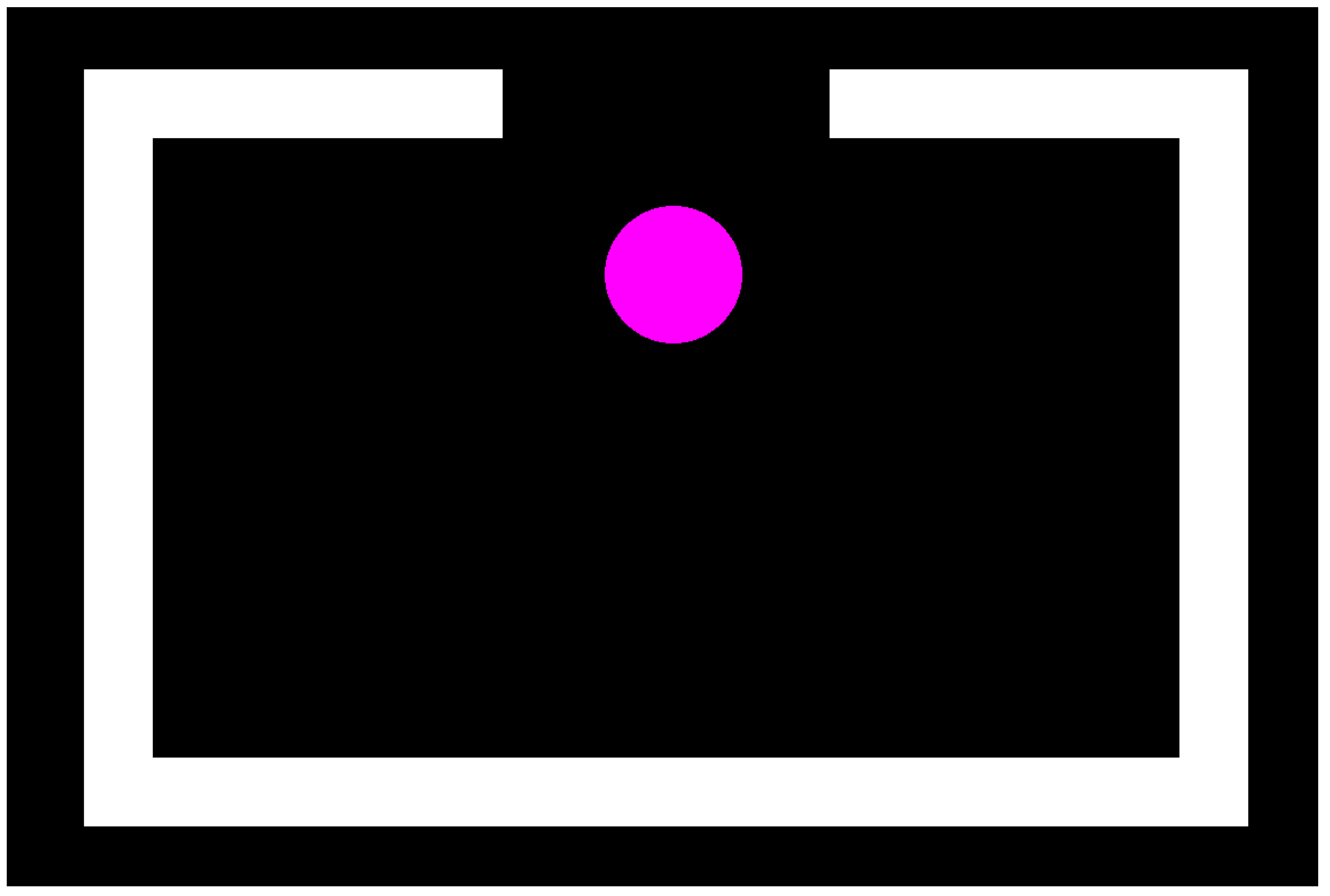
Figure 1 represents a simple room with one window and a person inside the room. The white lines represent the room’s walls, and the gap represents the window. A circle represents the person inside the room. The temperature simulation is initialized in the UAVEnv Python class. All the room’s walls are maintained at 15 °C, the person’s body temperature is 37 °C, the ambient temperature is simulated as 20 °C, and random noise is simulated as ±0.5 °C. Here, the person inside the room stands out because of a higher body temperature, the walls are cooler than the ambient temperature, and random noise adds realism to the temperature variations. The temperature gradient between the person, the walls, and the ambient environment is used to detect the person with an infrared camera.

The drone is created by loading a .bmp image file using Pygame’s ‘image.load’ function. Then, the rectangle for the drone is determined by PyGame’s ‘get_rect’ function, and the drone is positioned at the initial position for the UAV in the environment. The LiDAR and infrared camera are then initialized and visualized. Here, the LiDAR uses eight beams for observation.

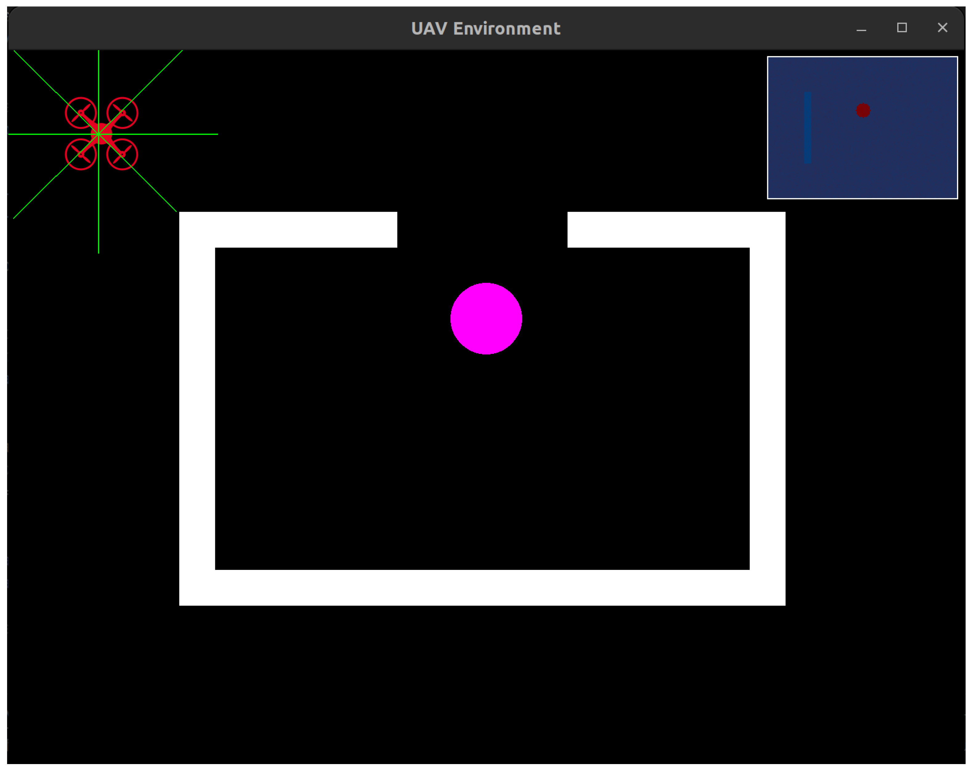
Figure 2 shows that the LiDAR originates from the drone’s center and is visualized as green lines. The drone is at its initial position. The rectangle in the upper-right corner of the figure represents the view from the infrared camera. The simulated LiDAR and infrared camera are mounted on the drone to collect data. The LiDAR sensor uses 8 beams, each separated by 45 degrees, with a maximum range of 200 pixels. Beams that do not intersect with any wall or obstacle within the 200-pixel range return the maximum value (200). The 8 LiDAR readings are normalized by dividing by the maximum range (200 pixels) before being fed to the network, yielding values in [0, 1]. The LiDAR beams are arranged in a star pattern, and each direction is represented as a vector. The UAV agent uses LiDAR beams to detect walls, maintain a safe distance, and make decisions about movement and path planning. The infrared camera image shows temperature variations as color-coded temperature variations. Hot areas appear redder, and cool areas appear bluer or greener. This visualization helps to understand what the UAV is seeing. The infrared camera is used for detecting people and fire spots in the environment.

The UAV motion function handles motion mechanics, collision avoidance, and wall-following behavior. The function stores the UAV agent’s current position, computes the distance to the nearest wall, and determines the angle between the UAV agent and the nearest wall. The UAV movement function implements dynamic speed control for the UAV agent. The base speed for the UAV agent is 10 pixels per step. The UAV agent’s speed decreases when it is close to the wall and approaches the wall at a poor angle. The UAV maintains base speed in optimal conditions. The UAV movement function supports four directional movements: up, down, left, and right. These movements correspond to actions 0, 1, 2, and 3, respectively. These discrete actions of the UAV agent are described in

Table 1. Description of the discrete actions of the UAV agent.

Layer Name	Input Size
Action 0	Move up—decrements the UAV’s y-coordinate by the current step size
Action 1	Move down—increments the UAV’s y-coordinate by the current step size
Action 2	Move left—decrements the UAV’s x-coordinate by the current step size
Action 3	Move right—increments the UAV’s x-coordinate by the current step size

. The UAV movement function also enforces environment boundaries so that the UAV agent does not go outside the bounds of the Pygame window. The UAV agent is bound to the X-axis from 0 to 1600 and the Y-axis from 0 to 1200.

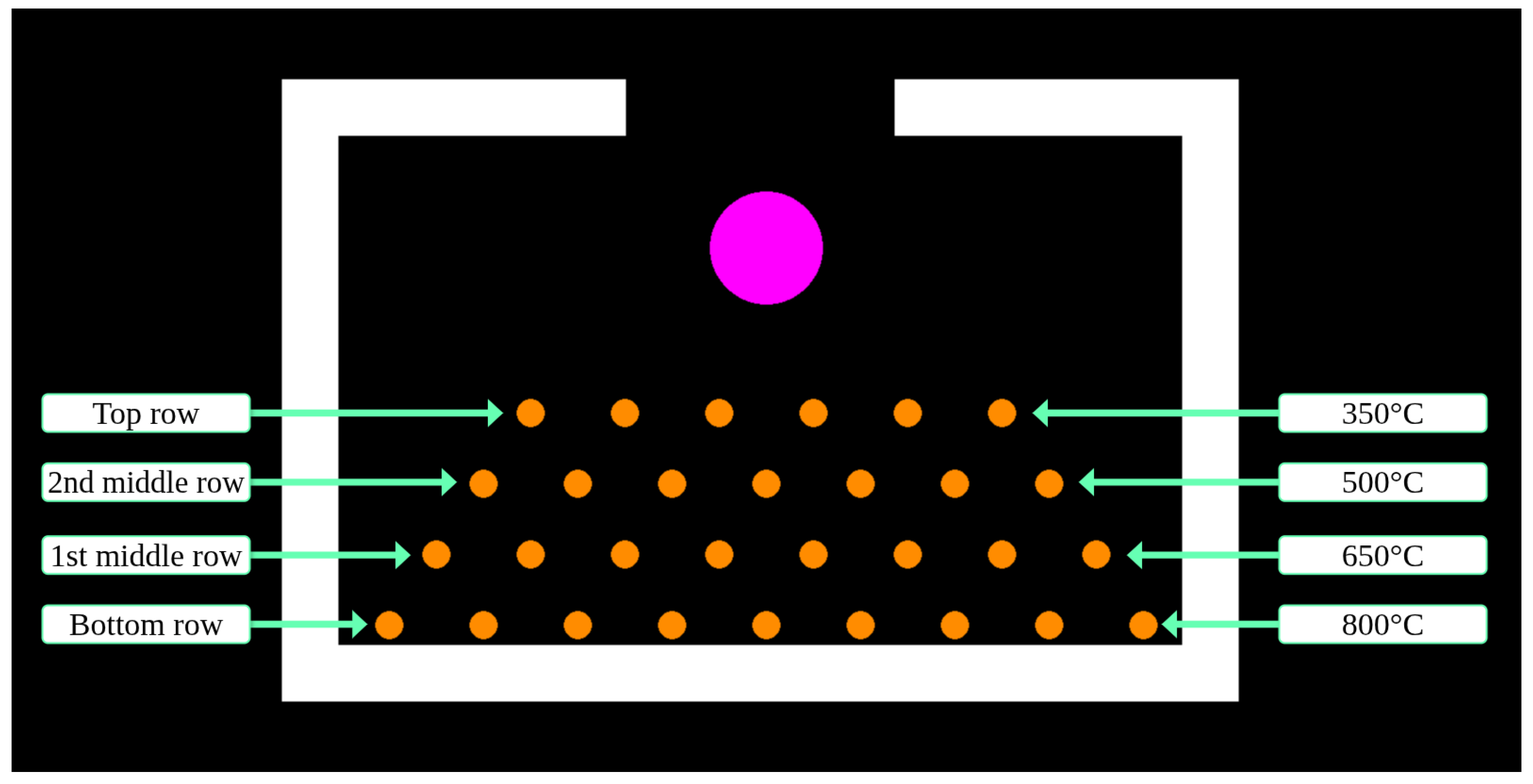
In this research, fire spots are simulated as rows. Figure 3 represents how the fire spots are simulated. The simulation has four rows of fire spots. These are the bottom, first middle, second middle, and top rows. These rows are simulated at different temperatures. The temperature values for the bottom, first, second, and top rows are 800 °C, 650 °C, 500 °C, and 350 °C, respectively. Here, the high temperature in the bottom row indicates that the fire is spreading from the bottom of the environment and gradually reaching the top, with the temperature decreasing. The fire rows are activated in the simulation according to the following sequence: bottom row → first middle row → second middle row → top row. The activation timing depends on the UAV agent’s actions. For the 4000-step limit simulations, the bottom row is active from the start. The first middle row activates after the UAV agent takes 1000 steps, the second middle row activates after the UAV agent takes 2000 steps, and lastly, the top row activates after the UAV agent takes 3000 steps. Similarly, for the 8000-step limit simulations, the bottom row is active from the start. The first middle row activates after the UAV agent takes 2000 steps, the second middle row activates after the UAV agent takes 4000 steps, and lastly, the top row activates after the UAV agent takes 6000 steps.

The DQN agents used in this research are initialized with parameters required for training. The parameters required for the DQN agents are listed in

Table 2. Training parameters for the DQN agents.

Parameters	Value
Discount factor	0.99
Learning rate	0.001
Training batch size	64
Replay buffer size (Transitions)	5000
Initial exploration rate	1
Minimum exploration rate	0.01
Exploration decay rate	0.995
Soft update parameter	0.001
Priority alpha	0.63
Priority beta	0.53
Priority beta increment	0.002
Priority epsilon	0.00001

.

The parameters of Prioritized Experience Replay (PER) control the prioritized sampling mechanism. The priority alpha determines the level of prioritization, priority beta controls the importance sampling weights, priority beta increment is the rate of beta increment, and priority epsilon is a small constant used to prevent zero priorities. N-step returns are implemented in the simulation to improve learning efficiency. This research uses a 3-step return calculation for the DQN agents. The n-step buffer uses a double-ended queue with a fixed maximum length. The Adam optimizer is used to train DQN agents.

3.1. Double DQN

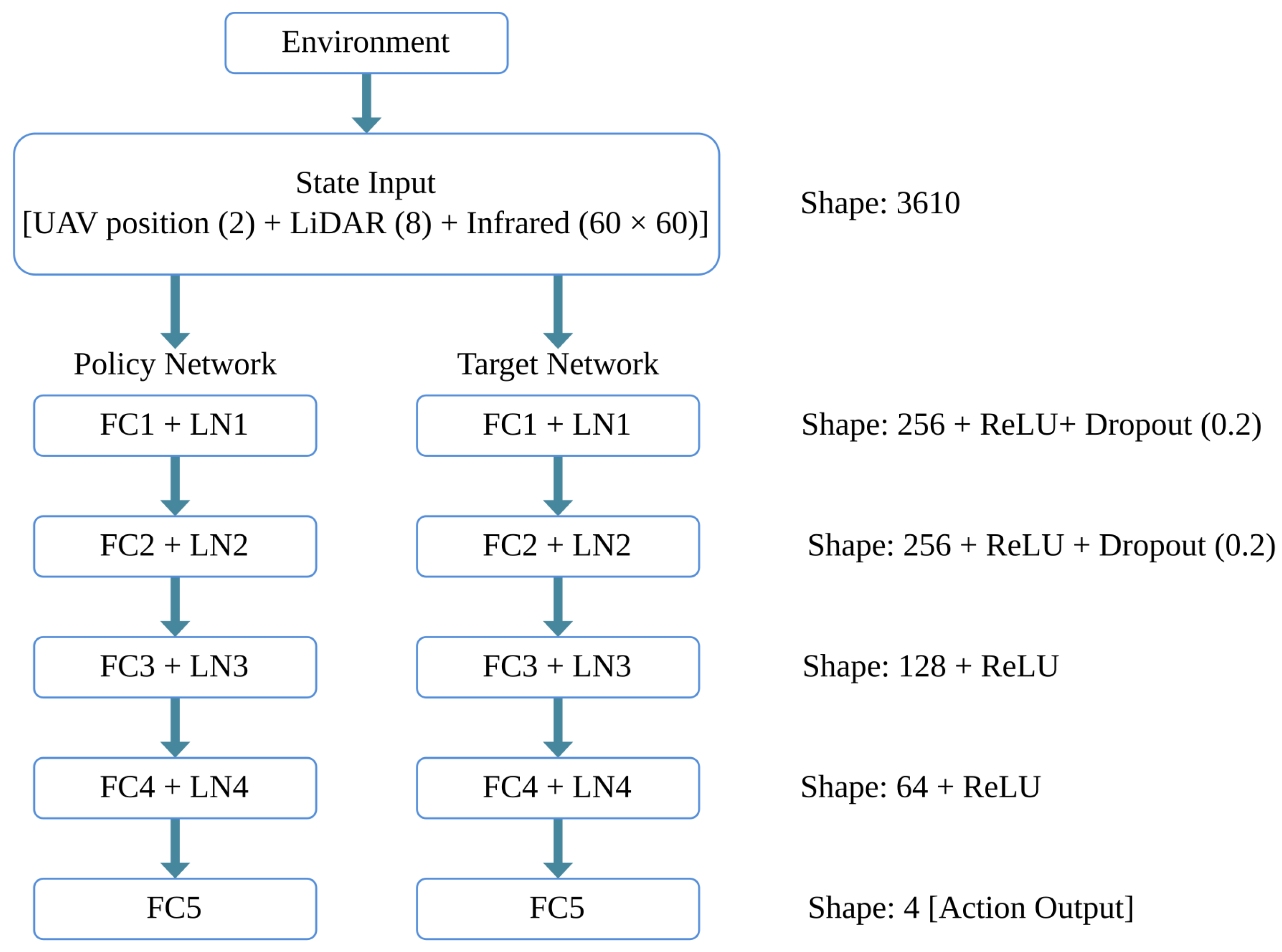
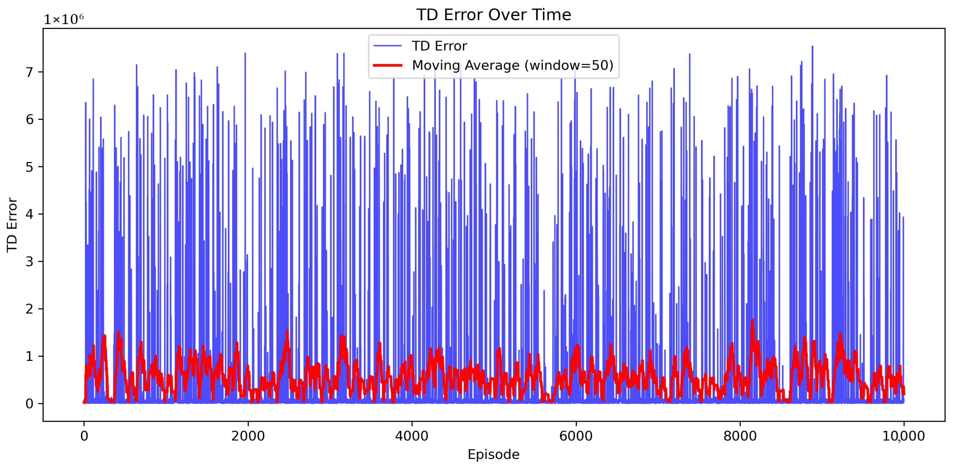
The structure of the Double DQN [62] is given in Figure 4. Here, FC represents a Fully Connected Layer, and LN represents a Normalization Layer. The input is taken from the simulation environment. The infrared camera output is downsampled from a 600 × 600-pixel grid to a 60 × 60-pixel grid using OpenCV’s cv2.resize() function with the default INTER_LINEAR (bilinear interpolation) flag. The complete state-vector breakdown is now documented as: UAV position (2 values: x, y in pixels) + LiDAR data (8 values, one per beam) + downsampled infrared camera (60 × 60 = 3600 values) = 3610 total features. The policy and target networks share the same neural network structure. The first fully connected network has a shape of 256, a ReLU activation function, a normalization layer, and a dropout probability of 20%. The second layer is similar to the first layer. The third layer has a shape of 128 and a ReLU activation function. The fourth layer has a shape of 64 and a ReLU activation function. The last layer is the output layer, which has a shape of 4. The outputs from both the policy and target networks are used to compute the Temporal Difference (TD) error. The TD error is utilized to select the training batch from Prioritized Experience Replay (PER). Both the policy network’s action outputs and the target network’s action outputs contribute to PER.

The summary of the layer sizes of Double DQN is described in

Table 3. Double DQN layer sizes summary.

Layer Name	Input Size	Output Size	Parameters
FC1	3610	256	924,416
LN1	256	256	512
FC2	256	256	65,792
LN2	256	256	512
FC3	256	128	32,896
LN3	128	128	256
FC4	128	64	8256
LN4	64	64	128
FC5	64	4	260

.

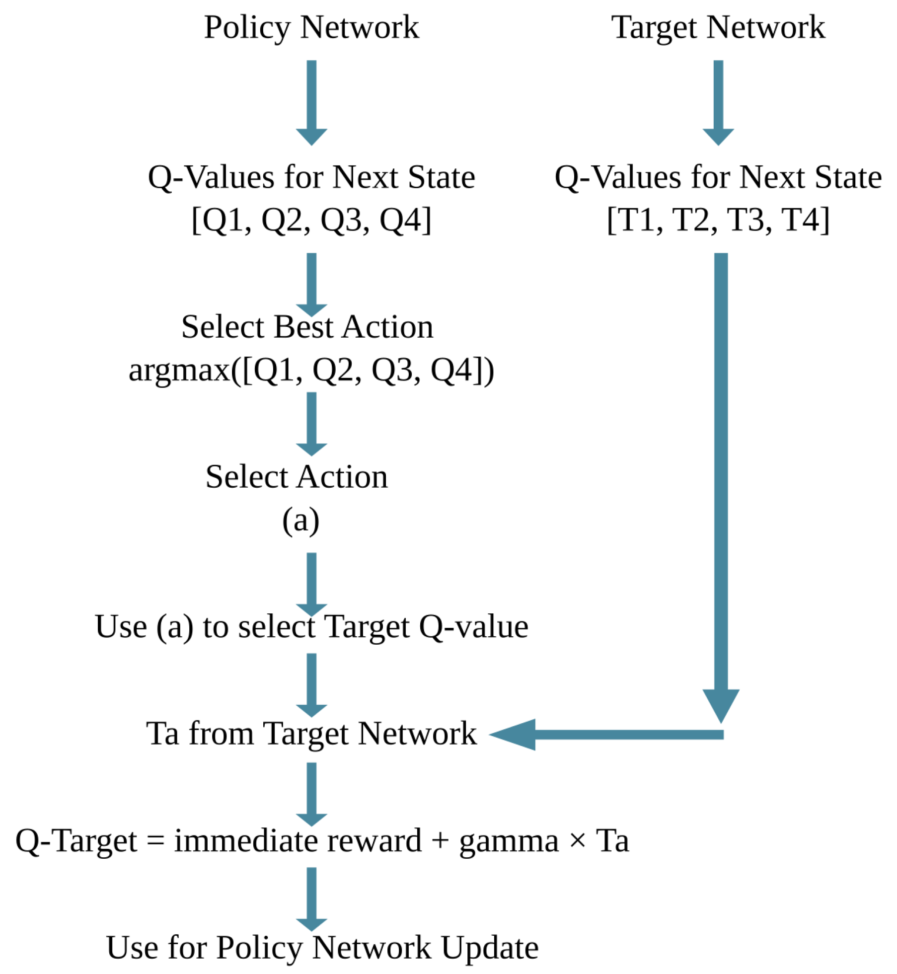
Figure 5 explains how two outputs from the policy and target networks are utilized. The training batch output of the PER is used to extract Q-values for the next-state values for both the policy and target networks. The policy network is used to select the best course of action. The target network is used to evaluate the best action. The final target Q-value is then computed. This separation between action selection and action evaluation is what makes Double DQN more stable than regular DQN, as it helps prevent the overestimation of Q-values that can occur when using a single network for both tasks. In Figure 5, gamma ($\gamma$) is the discount factor, which is set as 0.99 for this research. The discount factor determines how much future rewards are valued compared to immediate rewards by the DQN agent. In Figure 5, Ta is the target action value.

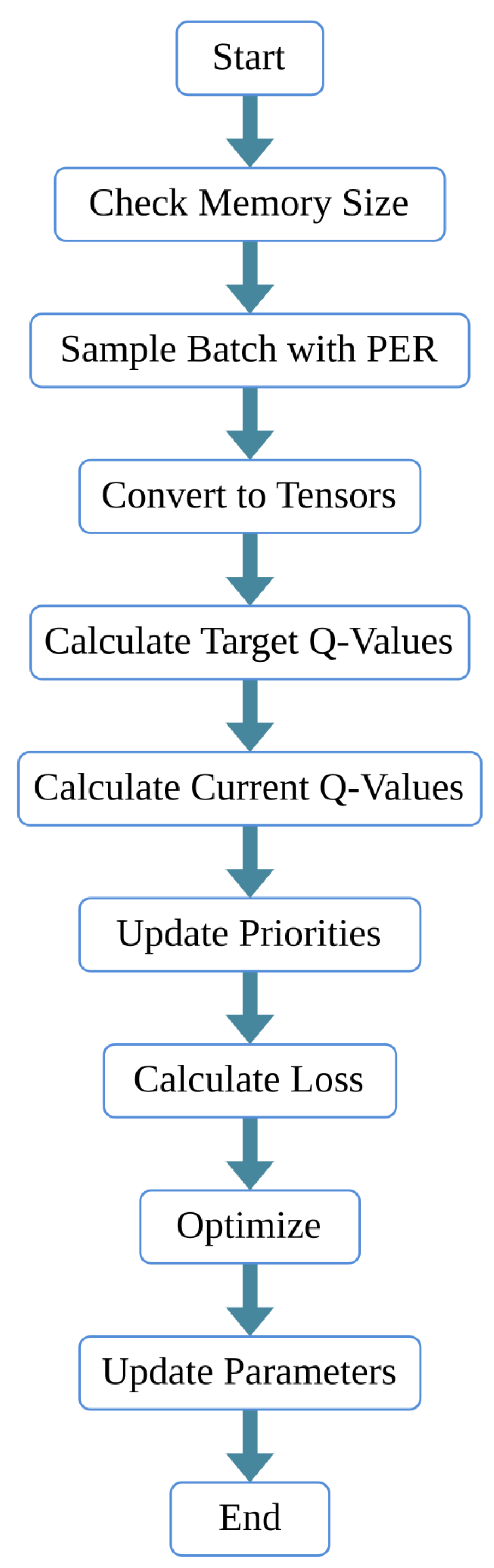
The flowchart of the training step function for the Double DQN is shown in Figure 6. The training step function implements the Double DQN for the UAV agent. The Double DQN algorithm uses two networks to decouple action selection from action evaluation. The final target Q value is then calculated using Equation (1).

$$Q_{\mathrm{target}}=R+\gamma Q_{\mathrm{target}}\left(s^{\prime },arg\underset{a^{\prime }}{max}{Q}_{\mathrm{policy}}(s^{\prime },a^{\prime })\right)$$

(1)

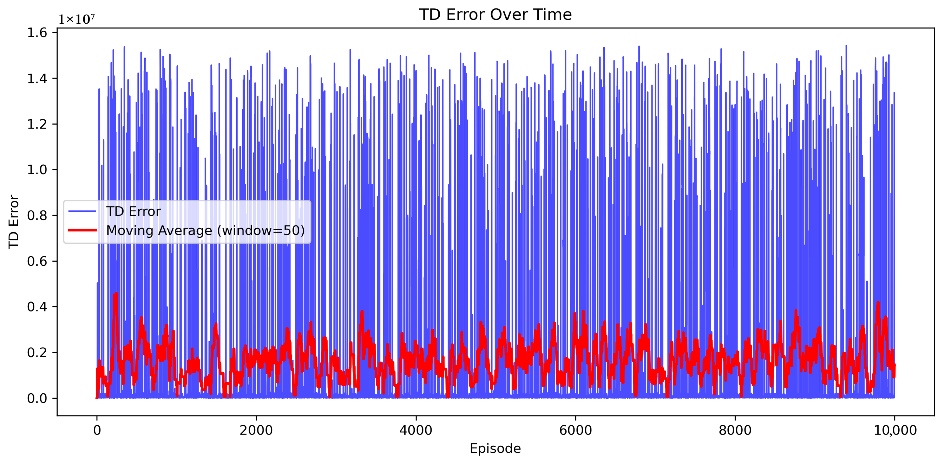
In Equation (1), R is the immediate reward, $\gamma$ is the discount factor, $Q_{\mathrm{target}}$ is the target network, $Q_{\mathrm{policy}}$ is the policy network, $s^{\prime }$ is the next state, and $a^{\prime }$ is the next action. The training step function at the beginning checks the memory size before training the model. If insufficient memory is found, it logs this for debugging purposes and skips the training process. Then, the function retrieves states, actions, rewards, next states, and episode completion data from the PER output. This function then converts these to PyTorch tensors for GPU acceleration. The function performs safety checks to see if the states and next states have the correct dimensions. If a dimension mismatch is found, the function raises an error. Then, the function uses the policy network to select the next actions and retrieves the corresponding Q-values from the target network. The function calculates the expected Q-values and gets the current Q-value from the policy network. The function then calculates the TD error to update the PER. This function then calculates the training loss and initiates the Adam optimizer. The function finally updates the PER beta and epsilon parameters.

3.2. Dueling DQN

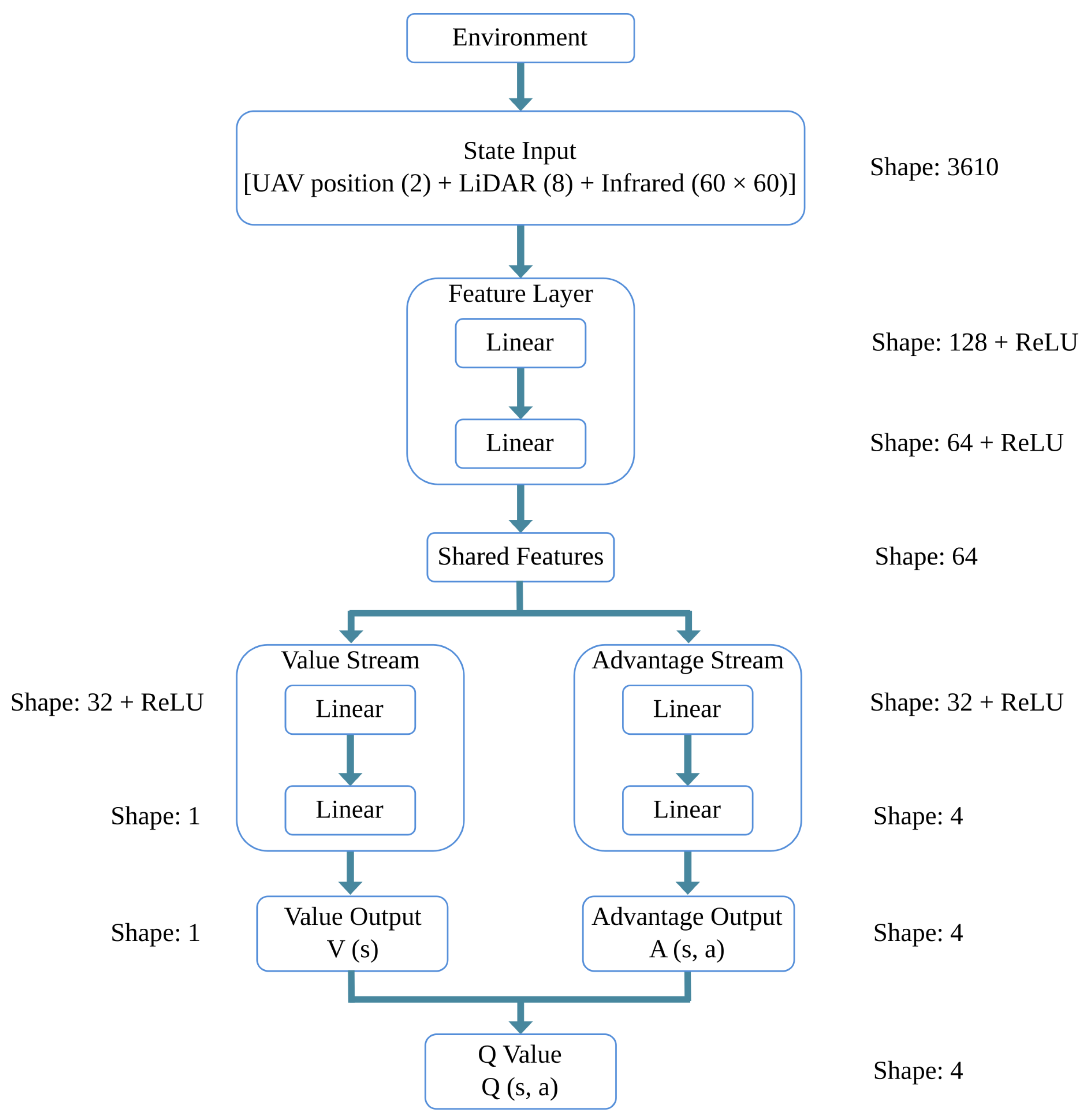
The structure of the Dueling DQN [63] is given in Figure 7. The input is taken from the simulation environment. The state input is an array that has a length of 3610. The input comprises the UAV position, LiDAR data, and downsampled infrared data. The dueling architecture is combined with PER for training. The feature is extracted for the simulated sensors using the feature layer. This feature layer comprises two linear neural network layers with ReLU activations. The first feature layer has a shape of 128, and the second feature layer has a shape of 64. The extracted features from the feature layers are fed to the value and advantage stream. The value stream has two linear neural network layers. The first linear layer has a shape of 32 and a ReLU activation function. The second linear layer has a shape of 1. The value output is taken from this layer. The advantage stream has two linear neural network layers. The first linear layer has a shape of 32 and a ReLU activation function. The second linear layer has a shape of 4. The output advantage is derived from this layer. The Q-value is calculated from the value and advantage output using Equation (2).

$$Q(s,a)=V\left(s\right)+A(s,a)$$

(2)

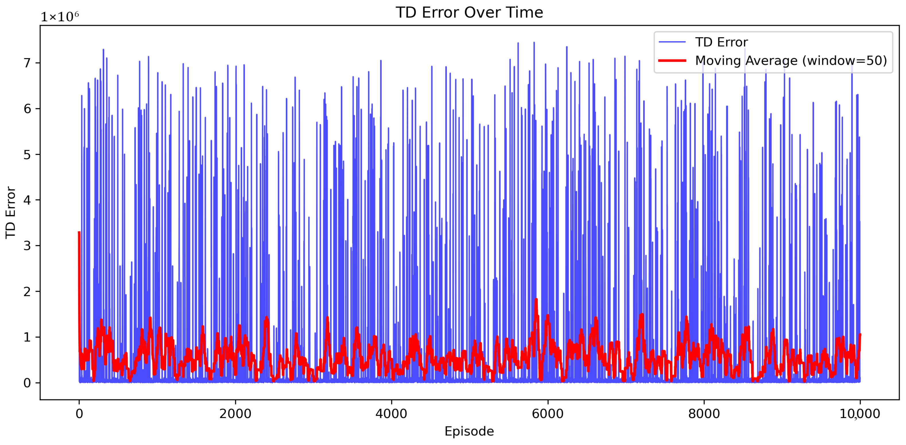
Here, $V\left(s\right)$ is the value output, and $A(s,a)$ is the advantage output. From the Q-value, the TD error is calculated. The TD error is utilized to select the training batch from PER.

Figure 7. The structure of the Dueling DQN.

Figure 7. The structure of the Dueling DQN.

The summary of the layer sizes is described in

Table 4. Dueling DQN layer sizes summary.

Layer Name	Input Size	Output Size	Parameters
Feature Layer 1	3610	128	462,208
Feature Layer 2	128	64	8256
Value Stream 1	64	32	2080
Value Stream 2	32	1	33
Advantage Stream 1	64	32	2080
Advantage Stream 2	32	4	132

.

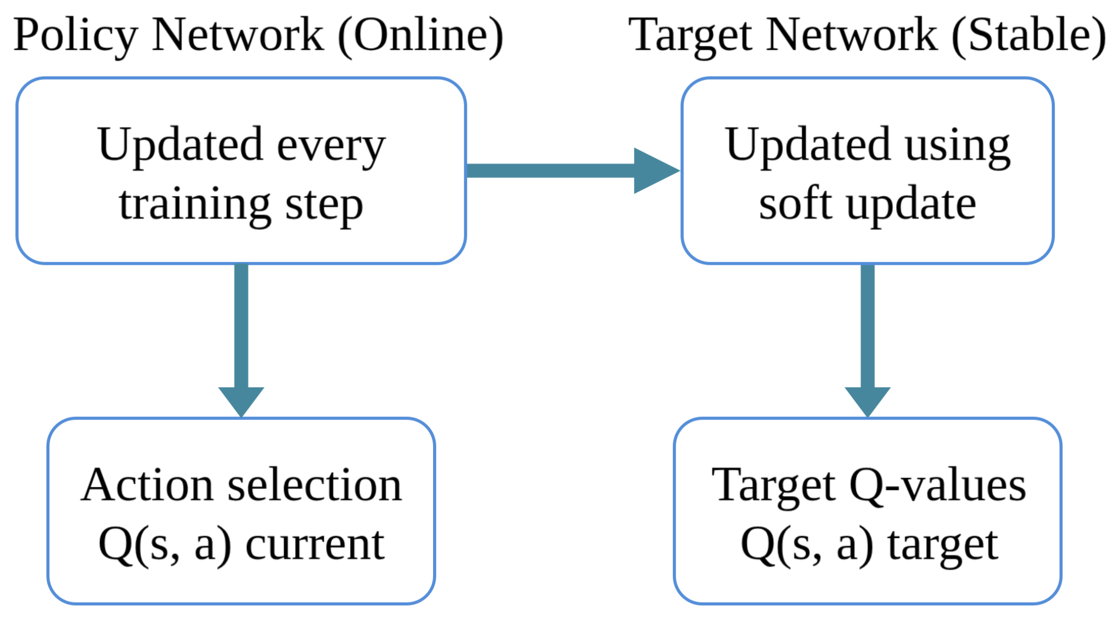
To understand how the training step function works, it is essential to understand how the policy and target networks operate within a Dueling DQN implementation. The flowchart of the interaction between these networks is given in Figure 8. Here, both policy and target network have the same structure as the Dueling DQN. The policy network is updated at the end of each episode, and the target network is updated using soft updates. Action selection is done from the Q-value output of the policy network, and target Q-values are obtained from the target network output.

The current Q-values are collected from the policy network. The state-action value refers to the Q-values associated with a given action. These are gathered from the current Q-value. The next-state values are obtained from the target network. The next action values are obtained from the policy network’s next-state value. The next Q-values are computed from the next-state values using the next-action values. The expected Q-values are calculated using Equation (3).

$$Q_{\mathrm{expected}}=R_t+(1-\mathrm{done})\times {\gamma }^n\times Q_{\mathrm{next}}$$

(3)

Here, $R_t$ is the reward, done is the episode end flag, $\gamma$ is the discount factor, which is 0.99. For this research, n is the value of n-steps, and $Q_{\mathrm{next}}$ is the next Q-values. The expected Q-values are computed by looking n-steps ahead to better handle delayed rewards.

For this research, the weights of the target network are updated using Polyak averaging, a soft update strategy that helps stabilize training in Deep Q-Learning. The soft update strategy is adopted here to reduce overestimation bias in Q-learning. The policy network learns actively from new experiences. The target network provides stable Q-value targets for training. The target network update function takes Tau ($\tau$) as input. Tau is a hyperparameter that controls the update rate. The value of Tau is set to 0.001 in the DQN models used in this research. The Polyak averaging is implemented using Equation (4). Here, ${\theta }_{\mathrm{target}}$ is the target network parameters, ${\theta }_{\mathrm{policy}}$ is the policy network parameters, and $\tau$ is the update rate parameter.

$${\theta }_{\mathrm{target}}=\tau \times {\theta }_{\mathrm{policy}}+(1-\tau )\times {\theta }_{\mathrm{target}}$$

(4)

3.3. D3QN

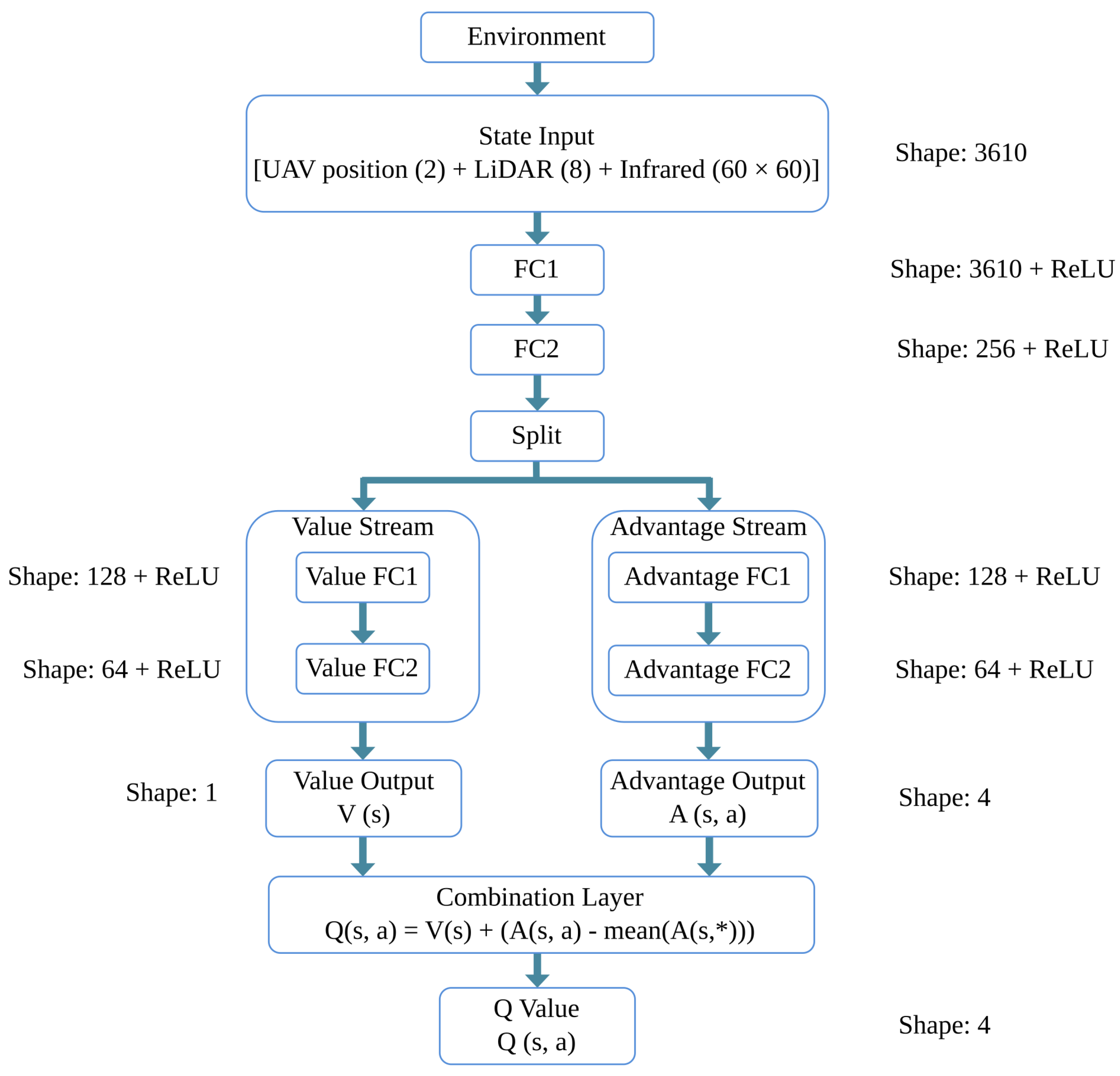
The structure of the D3QN is given in Figure 9. The input is taken from the simulation environment. The state input is an array that has a length of 3610. The input comprises the UAV position, LiDAR data, and downsampled infrared data. FC1 and FC2 are two fully connected layers with input shapes of 3610 and 256, respectively. Both layers use the ReLU activation function. The output of the FC2 layer is split into value stream and advantage stream. The value stream has two fully connected layers. The input shapes of these two layers are 128 and 64, respectively. These layers have a ReLU activation function. The advantage stream has similar fully connected layers. The value output and the advantage output are combined to get the Q-value.

The layer sizes are summarized in

Table 5. D3QN layer sizes summary.

Layer Name	Input Size	Output Size	Parameters
FC1	3610	256	924,160
FC2	256	128	32,896
Value FC1	128	64	8256
Value FC2	64	1	65
Advantage FC1	128	64	8256
Advantage FC2	64	4	260

.

The interaction between the target and policy networks is similar to that described in the Dueling DQN subsection. The next action values are taken from the policy network. The next Q-values are taken from the target network. The expected Q-values are calculated using Equation (3). The current Q-values are gathered from the policy network. The absolute TD error is calculated by subtracting the current Q-values from the expected Q-values. The loss is calculated from the current Q-values and the expected Q-values.

3.4. Prioritized Replay Buffer (PER)

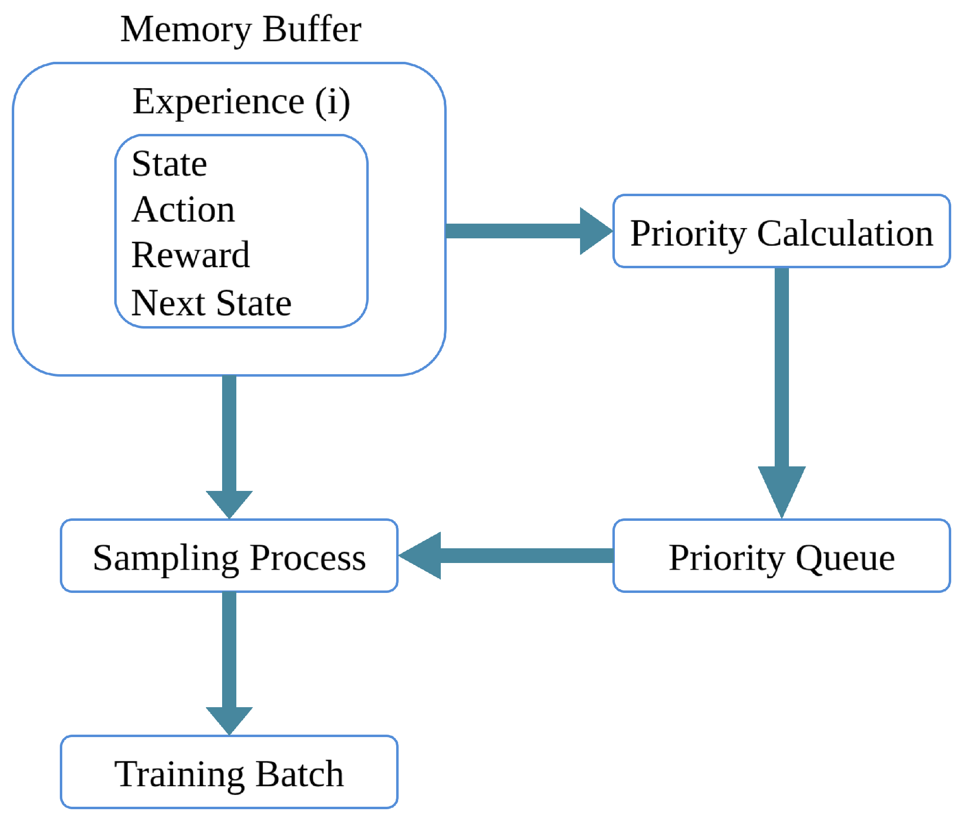
The working principle of PER [64] is illustrated in Figure 10. The DQN output is the action for the UAV Agent. The experiences are stored in the PER’s memory buffer. Then, the PER computes the transition priority (experience) and places it in the memory buffer queue. From this queue, transitions are sampled, and weights are assigned to each transition. Then, PER outputs a training batch, which is fed to the DQNs.

The prioritized replay buffer uses Temporal Difference (TD) error calculations to assign priorities to transitions. Equation (5) is used to compute the priority.

$$p_i=\left(\right|{\delta }_i+\epsilon {\left|\right)}^{\alpha }$$

(5)

Here, ${\delta }_i$ is absolute TD-error, $\epsilon$ is a small constant to ensure non-zero probability, and $\alpha$ is the PER parameter that controls how much prioritization is used.

This probability sampling transition is done by using Equation (6)

$$P\left(i\right)={\displaystyle \frac{p_i}{{\sum }_k{p}_k}}$$

(6)

Here, $P\left(i\right)$ is the probability of sampling transition i, $p_i$ is the priority of transition i, and ${\sum }_k{p}_k$ is the sum of all priorities in the buffer.

The sampling weight is applied to a transition by PER. The Equation (7) is used for sampling.

$$w_i={\left({\displaystyle \frac{1}{N}}\times {\displaystyle \frac{1}{P\left(i\right)}}\right)}^{\beta }$$

(7)

Here, $w_i$ is the sampling weight of the transition, N is the memory size, and $\beta$ is the PER parameter.

Algorithm 1 presents the complete DQN training loop and is structured around two visually distinct pathways to directly address the conceptual separation between action selection and experience replay. The action-selection pathway, executed at every environment step, uses a standard $\epsilon$-greedy policy derived solely from the output of the policy network $Q_{{\theta }_{\mathrm{policy}}}$, with $\epsilon$ initialized at $1.0$ and decayed by a factor of $0.995$ per episode to a minimum of $0.01$ as specified in Table 2. PER appears nowhere in this pathway. Once an action is executed and a transition is collected, the n-step buffer accumulates experiences over $n=3$ steps, then computes the 3-step discounted return $R_t$ and stores the resulting transition in the PER buffer $\mathcal{B}$ with maximum initial priority.

The training pathway, executed only when $\left|\mathcal{B}\right|$ contains at least one full mini-batch, is where PER exclusively operates: it samples a batch of 64 transitions according to the priority distribution $P\left(i\right)=p_i^{\alpha }/{\sum }_k{p}_k^{\alpha }$ with $\alpha =0.63$ from Equation (6), and assigns importance-sampling weights $w_i$ with $\beta =0.53$ incrementing by $0.002$ per update step to correct for the sampling bias introduced by prioritization in Equation (7). Target Q-values are then computed following the Double DQN rule, where the policy network selects the next action and the target network evaluates its value using Equations (1) and (3), after which the TD error ${\delta }_i$ drives both the importance-weighted loss minimized by the Adam optimizer and the priority update back into $\mathcal{B}$ via $p_i={({\delta }_i+{\epsilon }_{\mathrm{PER}})}^{\alpha }$ with ${\epsilon }_{\mathrm{PER}}=0.00001$ using Equation (5).

Finally, the target network weights are updated softly via Polyak averaging with $\tau =0.001$, as in Equation (4). This structure makes explicit that PER exclusively governs which stored transitions are used for gradient computation and plays no role whatsoever in how the agent selects actions during interaction with the environment.

3.5. Reward Function

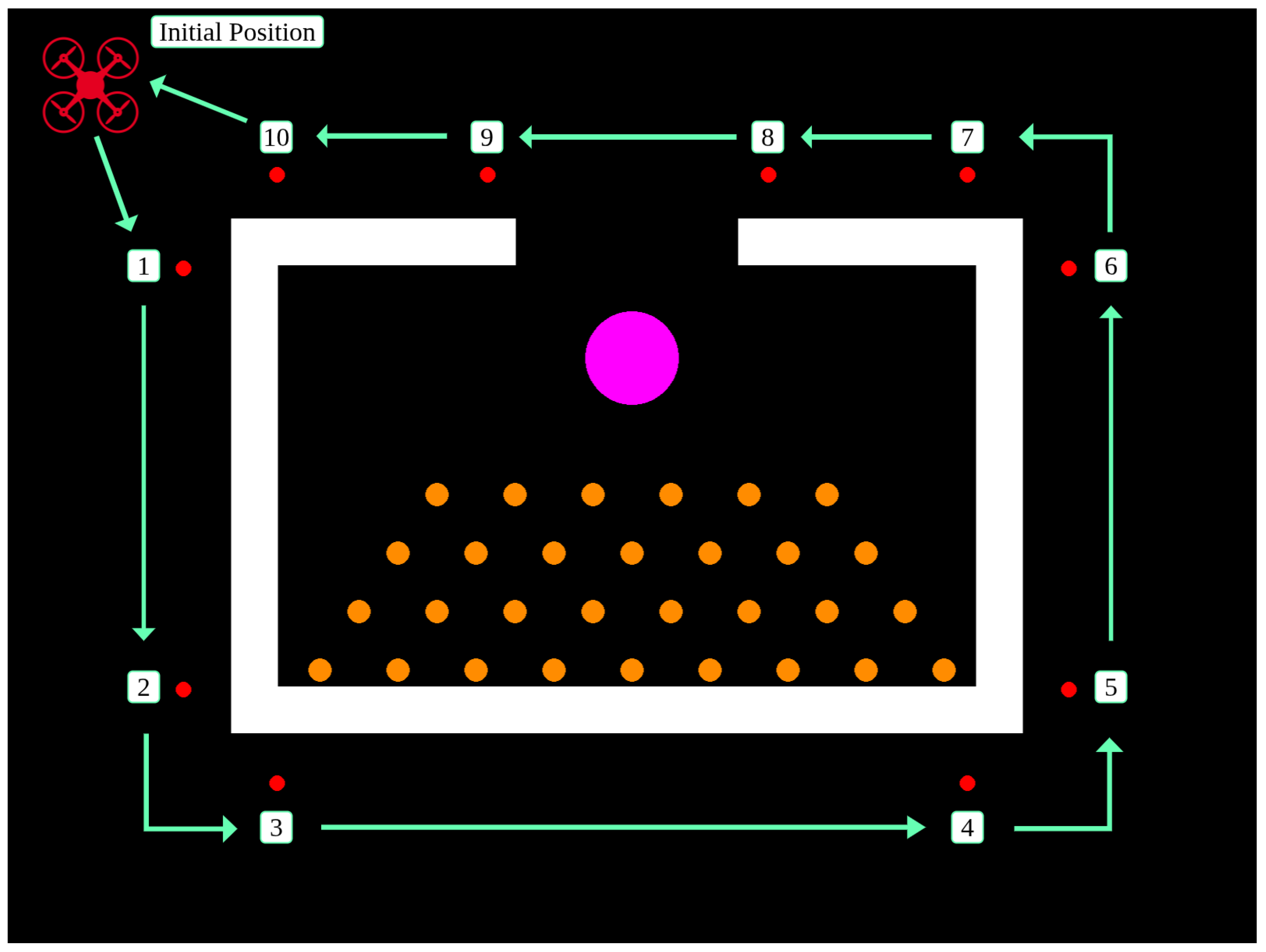
The reward or step function processes the UAV agent’s actions, updates the environment state, and calculates rewards or penalties for the UAV agent. It takes the UAV’s action as an input and returns the next state, reward, done flag, and an empty dictionary for additional info. The empty dictionary adheres to the gym environment standards. Initially, the function initializes the episode status and stores the UAV agent’s current position and the distance to the wall for future reference. The UAV agent’s position is updated based on the action, and a small negative reward is used to encourage efficient path completion. The mission is considered complete if the UAV agent visits all checkpoints, detects the person, and returns to its initial position. The checkpoint implementation for the UAV agent is illustrated in Figure 11 and Figure 12.

Algorithm 1 DQN Training Loop with Prioritized Experience Replay (PER)
1 Initialize:      Policy network $Q_{{\theta }_{\mathrm{policy}}}$ with random weights ${\theta }_{\mathrm{policy}}$      Target network $Q_{{\theta }_{\mathrm{target}}}$ with ${\theta }_{\mathrm{target}}\leftarrow {\theta }_{\mathrm{policy}}$      PER buffer $\mathcal{B}$ with capacity $N=5000$;   n-step buffer (deque, $n=3$)      $\epsilon \leftarrow 1.0$,   ${\epsilon }_{\min }\leftarrow 0.01$,   ${\epsilon }_{\mathrm{decay}}\leftarrow 0.995$      $\gamma \leftarrow 0.99$,   $\tau \leftarrow 0.001$,   batch size $\leftarrow 64$      $\alpha \leftarrow 0.63$,   $\beta \leftarrow 0.53$,   ${\beta }_{\mathrm{inc}}\leftarrow 0.002$,   ${\epsilon }_{\mathrm{PER}}\leftarrow 0.00001$
2 for  $\mathrm{episode}=1$ to $10,000$ do
3      $s\leftarrow \mathtt{environment}.\mathtt{reset}\left(\right)$	$▹s=\left[\mathrm{pos}\right(2),\mathrm{LiDAR}(8),\mathrm{IR}(3600\left)\right]$
4      for each step do
5            ACTION-SELECTION PATHWAY (online)—PER is NOT involved here
6            if $\mathtt{random}\left(\right)<\epsilon$ then
7              $a\leftarrow \mathrm{random}\mathrm{action}$	▹ explore
8            else
9              $a\leftarrow arg{max}_{a^{\prime }}{Q}_{{\theta }_{\mathrm{policy}}}(s,a^{\prime })$	▹ exploit via $\epsilon$-greedy over policy network output
10          end if
11          $s^{\prime },r,\mathrm{done}\leftarrow \mathtt{environment}.\mathtt{step}\left(a\right)$	▹ execute action
12          Store $(s,a,r,s^{\prime },\mathrm{done})$ in n-step buffer
13          if n-step buffer is full then
14              Compute 3-step return $R_t={\sum }_{k=0}^2{\gamma }^k{r}_{t+k}$
15              Store $(s_t,a_t,R_t,s_{t+3},\mathrm{done})$ in $\mathcal{B}$ with max priority	▹ new transitions get max priority by default
16          end if
17          $s\leftarrow s^{\prime }$
18          TRAINING PATHWAY (offline)—PER is ONLY involved here
19          if $\left|\mathcal{B}\right|\ge \mathrm{batch}\mathrm{size}$ then
20              $\{(s_i,a_i,R_i,s_i^{\prime },{\mathrm{done}}_i),w_i\}\leftarrow \mathcal{B}.\mathtt{sample}(\mathrm{batch}=64)$
PER samples by $P\left(i\right)=p_i^{\alpha }/{\sum }_k{p}_k^{\alpha }$;   importance weights $w_i={\left(\frac{1}{N·P\left(i\right)}\right)}^{\beta }$
— Compute target Q-values (Double DQN rule) —
21             $a_i^{\ast }\leftarrow arg{max}_{a^{\prime }}{Q}_{{\theta }_{\mathrm{policy}}}(s_i^{\prime },a^{\prime })$	▹ action selected by policy network
22             $Q_{\mathrm{next}}\leftarrow Q_{{\theta }_{\mathrm{target}}}(s_i^{\prime },a_i^{\ast })$	▹ value evaluated by target network
23             $Q_{\mathrm{expected}}\leftarrow R_i+(1-{\mathrm{done}}_i)·{\gamma }^n·Q_{\mathrm{next}}$	▹ Equation (3)
— Compute current Q-values —
24             $Q_{\mathrm{current}}\leftarrow Q_{{\theta }_{\mathrm{policy}}}(s_i,a_i)$
— TD error and importance-weighted loss —
25             ${\delta }_i\leftarrow \left|Q_{\mathrm{expected}}-Q_{\mathrm{current}}\right|$
26             $\mathcal{L}\leftarrow {\displaystyle \frac{1}{\left|\mathcal{B}\right|}}{\sum }_i{w}_i·{\delta }_i^2$	▹ importance-weighted loss
— Update policy network —
27             Backpropagate $\mathcal{L}$ via Adam optimizer
— Update PER priorities —
28             $p_i\leftarrow {({\delta }_i+{\epsilon }_{\mathrm{PER}})}^{\alpha }$	▹ Equation (5);   ${\epsilon }_{\mathrm{PER}}=0.00001$
29             $\mathcal{B}.\mathtt{update}\_\mathtt{priorities}\left(p_i\right)$
— Soft-update target network (Polyak averaging) —
30             ${\theta }_{\mathrm{target}}\leftarrow \tau {\theta }_{\mathrm{policy}}+(1-\tau ){\theta }_{\mathrm{target}}$	▹ Equation (4);   $\tau =0.001$
— Update PER β —
31             $\beta \leftarrow min\left(1.0,\beta +{\beta }_{\mathrm{inc}}\right)$	▹${\beta }_{\mathrm{inc}}=0.002$
32          end if
33          if done then break
34          end if
35      end for
36      $\epsilon \leftarrow max({\epsilon }_{\min },\epsilon ·{\epsilon }_{\mathrm{decay}})$	▹ decay exploration rate after each episode
37 end for

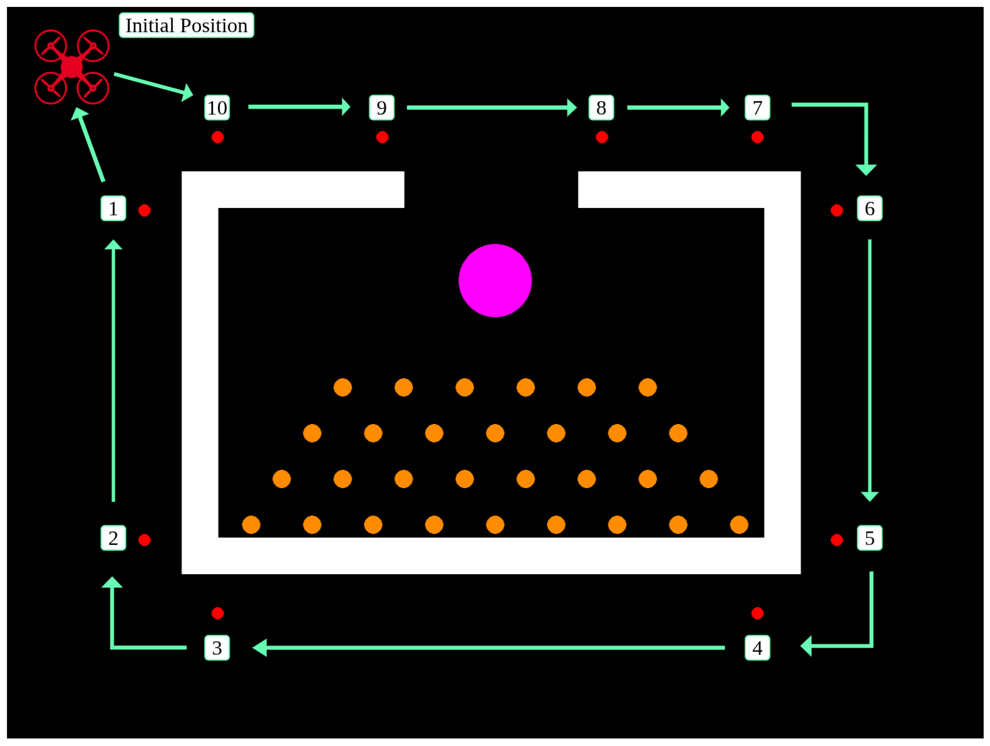
In Figure 11 and Figure 12, the UAV agent is in its initial position. The coordinates of the UAV agent’s initial position are (100, 100). The UAV agent starts every episode from the initial position. The checkpoints are shown as red dots in Figure 11 and Figure 12. The order of the checkpoints is numbered in the figures. The checkpoints are sequentially activated and deactivated by the reward function. At the start of an episode, only checkpoints 1 and 10 are active. The UAV agent can receive a reward only by visiting one of the two checkpoints. Based on the UAV agent’s motion, the remaining checkpoints are activated. The UAV agent can follow either ’forward’ or ’backward’ movement. The forward movement checkpoint activation sequence is represented in Figure 11, and the backward movement checkpoint activation sequence is represented in Figure 12.

If the UAV agent reaches checkpoint 1 first, it must then proceed with the forward motion. In this scenario, after reaching checkpoint 1, all the other checkpoints except checkpoint 2 will be inactive. The checkpoint activation sequence for forward movement is 2 → 3 → 4 → 5 → 6 → 7 → 8 → 9 → 10 → initial position. During the UAV agent’s forward movement, checkpoints are deactivated sequentially. For example, after the UAV agent crosses checkpoint 1, it will be deactivated, checkpoint 2 will be active, and so on. Only one checkpoint will be active at a time, and the UAV agent will decide whether to move forward or backward.

If the UAV agent reaches checkpoint 10 first, it must then follow the backward movement. In this scenario, after reaching checkpoint 10, all the other checkpoints except checkpoint 9 will be inactive. The checkpoint activation sequence for backward movement is 9 → 8 → 7 → 6 → 5 → 4 → 3 → 2 → 1 → initial position. During the UAV agent’s backward movement, checkpoints are deactivated sequentially. For example, after the UAV agent crosses checkpoint 10, it will be deactivated, checkpoint 9 will be active, and so on.

The reward and penalty conditions are explained in

Table 6. Basic navigation rewards.

Action/Achievement	Reward Value	Condition
Basic Step	$-1$	Each action taken
Checkpoint 1	+1000	Reaching first checkpoint
Checkpoint 2	+2000	Cumulative reward for reaching second checkpoint
Checkpoint 3	+3000	Cumulative reward for reaching third checkpoint
Checkpoint 4	+4000	Cumulative reward for reaching fourth checkpoint
Checkpoint 5	+5000	Cumulative reward for reaching fifth checkpoint
Checkpoint 6	+6000	Cumulative reward for reaching sixth checkpoint
Checkpoint 7	+7000	Cumulative reward for reaching seventh checkpoint
Checkpoint 8	+8000	Cumulative reward for reaching eighth checkpoint
Checkpoint 9	+9000	Cumulative reward for reaching ninth checkpoint
Checkpoint 10	+10,000	Cumulative reward for reaching tenth checkpoint

,

Table 7. Progress bonuses.

Achievement	Bonus Value	Condition
Checkpoint Progress	+500 × N	N = checkpoint number (0–9)
Person Detection	+1000	First time detecting person
Mission Completion	+10,000	Return to start after objectives

,

Table 8. Wall-following rewards.

Behavior	Reward Formula	Condition
Optimal Distance	+20 × accuracy	Within wall following tolerance (20 pixels)
Good Angle	+30 × angle accuracy	Within angle tolerance (15°)
Stable Distance	+10 × stability	Distance change < 10 pixels
Stable Angle	+10 × angle stability	Angle change < tolerance

,

Table 9. Penalties.

Violation	Penalty Value	Condition
House Collision	$-500$	Flying inside house bounds
Person Collision	$-800$	Too close to person
Wrong Checkpoint	$-2000$	Attempting inactive checkpoint
Too Close to Wall	$-50$ × ${(1-\mathrm{closeness}\mathrm{ratio})}^2$	Closer than follow distance
Too Far from Wall	$-30$ × distance ratio	Farther than follow distance
Poor Wall Angle	$-20$ × ${\left({\displaystyle \frac{\mathrm{angle}\mathrm{tolerance}}{90}}\right)}^2$	Angle exceeds tolerance

,

Table 10. Distance-based rewards.

Condition	Formula	Description
To Checkpoint	${\displaystyle \frac{1000}{(1+\mathrm{distance})\times (\mathrm{checkpoint}+1)}}$	Moving toward active checkpoint
Return to Start	${\displaystyle \frac{500}{(\mathrm{distance}\mathrm{to}\mathrm{start}+1)}}$	After visiting all checkpoints

and

Table 11. Fire interaction rewards and penalties.

Interaction Type	Distance Range	Reward/Penalty
Collision	<25 pixels	$-1000$ × ${\displaystyle \frac{\mathrm{temperature}}{800}}$
Heat Damage	25–50 pixels	$-200\times {\displaystyle \frac{\mathrm{temperature}}{800}}\times (1-{\displaystyle \frac{\mathrm{distance}}{50}})$
Detection	50–100 pixels	$+100\times {\displaystyle \frac{\mathrm{temperature}}{800}}\times (1-{\displaystyle \frac{\mathrm{distance}}{50}})$
New Fire Discovery	<100 pixels	$+500\times {\displaystyle \frac{\mathrm{temperature}}{800}}$

.

The basic navigation rewards are described in Table 6. The UAV agent receives a −1 penalty for each step it takes. This small negative reward encourages the UAV agent to take only steps that lead to positive rewards. The table above shows the forward motion patterns of the UAV. Upon reaching checkpoint 1, the UAV agent receives a +1000 reward. Then, at checkpoint 2, the cumulative reward for following the active checkpoints is 2000. The maximum cumulative reward the agent can get for passing through all the checkpoints sequentially is 10,000. The checkpoint sequence reverses when the UAV agent chooses the backward movement pattern. In this scenario, the UAV agent receives a +1000 reward upon passing through checkpoint 10 and accumulates a total of 2000 rewards after passing through checkpoint 9, and so on.

Table 7 describes the progress bonuses for the UAV agent. The UAV agent gets a bonus after crossing a checkpoint. In the Table 7, N is the number of active checkpoint the UAV has crossed. The reward increases with the number of active checkpoints crossed by the UAV agent. The UAV agent receives +1000 points, which serves as a bonus for detecting the person inside the house. The UAV agent can receive this person-detection reward only once per episode. The UAV agent receives a substantial reward of +10,000 upon completing the mission. Mission completion requires the UAV to visit all checkpoints in sequence (forward or backward), detect a person inside the house, and return to its initial position.

The UAV agent’s wall-following rewards are described in Table 8. The UAV agent is rewarded for maintaining the optimal distance from the wall. The reward amount is based on accuracy for maintaining the optimal distance from the wall. The UAV agent also gets rewarded for maintaining a good angle to the wall. The UAV agent should maintain a 45° angle to the wall while following it. The good-angle reward is computed based on the angle accuracy when following the wall. The UAV agent also gets rewards for maintaining a stable distance and stable angle while following the wall. The UAV agent should maintain a distance of 100 pixels from the wall. If the UAV agent follows the wall, maintaining a distance within 10 pixels of 100, the UAV agent is rewarded in each step for a stable distance from the wall. The UAV agent also receives a reward for maintaining a stable angle. If the angle change from 45° is less than the angle tolerance, then the UAV agent will be rewarded at every step.

Table 9 lists the penalties given to the UAV agent by the reward function. If the UAV agent enters the house, it incurs a 500-point penalty for colliding with the house. If the UAV agent gets too close to the person, it gets an 800-point penalty. If the UAV agent breaks the sequence while traversing the checkpoints or attempts to fly toward an inactive checkpoint, it incurs a 2000-point penalty. The UAV agent gets penalties for being too close to the wall, too far from the wall, and having a poor angle to the wall. These penalties are computed using the closeness ratio, the distance ratio, and the angle tolerance, respectively. Here, the closeness ratio is the current distance from the wall divided by 100 pixels, the distance ratio is the current distance from the wall - 100 pixels divided by 100 pixels, and the angle tolerance is 15 degrees.

Table 10 describes the dynamic rewards given to the UAV agent by the reward function based on distance. UAV agents get a dynamic reward for moving towards an active checkpoint. This reward encourages the UAV agent to go towards the active checkpoint. The formula for movement toward the checkpoint reward is given in Table 10. After visiting all checkpoints in sequence, the UAV agent receives an additional dynamic reward for returning to its initial position. The formula for this reward is given in Table 10. This reward is given to the UAV agent to encourage movement towards the initial position.

Table 11 describes the rewards and penalties for the UAV agent for interacting with the fire spots. If the UAV agent’s distance is less than 25 pixels from the fire spot, it is considered a collision, and a penalty is given according to the temperature of the fire spot. If the UAV agent is within 25 to 50 pixels of a fire spot, it is considered that the UAV agent has sustained fire damage, and a penalty is given based on the temperature of the fire spot and the distance from the fire spot. The equation for the penalty is given in Table 11. The UAV agent gets a one-time reward for detecting a fire spot for the first time. This reward is based on the temperature of the fire spot that the UAV agent discovers. The higher the temperature, the greater the reward. The UAV agent receives rewards for detecting fire spots based on their temperature and distance. The equation for the fire spot detection reward is given in Table 11.

The reward function terminates an episode when the episode limit is reached or the mission is complete. UAV agents take a limited number of steps to simulate a battery. The reward function sets the step limit for this step. An episode also ends if the UAV agent completes the mission. The condition for mission completion is that the UAV visits all the checkpoints in sequence (forward or backward), locates the person inside the house, and returns to its initial position.

4. Results

Experiments with all DQN models for the UAV agent were conducted under four training conditions. Each training condition had 10,000 episodes.

Table 12. Conditions for the experiments for Double DQN, Dueling DQN, and D3QN.

Condition	Steps Limit	Number of Processes	Memory per Process (Gigabytes)
1	4000	4	50
2	4000	1	200
3	8000	2	100
4	8000	1	200

explains the conditions of the experiments.

4.1. Epsilon Decay over Episodes

The epsilon decay over episodes graph is ubiquitous across all DQN agents. Here, epsilon is the exploration rate, and epsilon changes throughout training in the DQN algorithm. The rate of change in epsilon over the episodes’ graph is shown in Figure 13.

The epsilon value starts at 1 to encourage the UAV agent to explore the environment; it eventually stabilizes near 0.01 to encourage the UAV agent to exploit what it has learned from exploration. Figure 13 depicts the epsilon value change over 10,000 episodes. When the epsilon is close to 1.0, the agent mostly takes random actions to explore the environment. As epsilon decreases, the agent gradually shifts from an exploration to an exploitation strategy. When the epsilon value reaches 0.01, the agent primarily exploits its learned knowledge while maintaining a small probability of exploration.

4.2. Double DQN

The experiments with the Double DQN model for the UAV agent were conducted under the training conditions mentioned in Table 12. The cumulative reward distribution across episodes for all experimental conditions is shown in Figure 14, Figure 15, Figure 16 and Figure 17.

In Figure 14, the UAV agent starts with a zero reward, then finds an initial policy, and the reward jumps to ~20,000 points relatively early in training. The UAV agent continually found better strategies for completing the goal, as the cumulative reward increased. Around episode 1000, the UAV agent reached over 40,000 reward points and achieved a better policy. Just before reaching 2000 episodes, the UAV agent improved its policy again, achieving 50,000 reward points. Afterward, the UAV agent found a better policy after 5000 episodes, and the cumulative reward increased to ~55,000 points. After that, the UAV agent gradually improved its policy and eventually reached 60,000 reward points, just before completing 10,000 episodes. This indicates that the agent has identified an optimal policy for a successful episode.

In Figure 15, the UAV agent starts training from a very low reward of ~3.5 million negative reward points. This low reward indicates that the UAV agent made many mistakes at the start of training and incurred increasingly severe penalties. From the analysis of the output data, it is evident that the reward increased sharply to 56,700 points and remained at this level for the remainder of the training. This sharp rise in reward indicates that the UAV agent has found an initial policy for successful episodes early in training and has adhered to it for the remainder of training, without significant improvement to the policy.

In Figure 16, the UAV agent starts training with a negative ~200,000 reward points. The high negative reward indicates that the UAV agent made mistakes and followed the wrong policy. The reward sharply increased to 25,000 points early in training, indicating that the UAV agent had found an initial policy for successful episodes. The reward points increased gradually to 50,000 over 2000 episodes, indicating that the UAV agent had improved the initial policy and avoided major penalties. Upon analyzing the output data, we observe that for the remainder of the training, the UAV agent gradually improves its policy, resulting in successful episodes and achieving a maximum reward of 63,000 points.

In Figure 17, the UAV agent starts training with a negative ~180,000 reward points. At the start of the training, the UAV agent made numerous mistakes and incurred substantial penalties. In the early stages of training, the UAV agent’s reward points increased to ~25,000, indicating that the agent had discovered an initial policy for successful episodes. Around episode 1000, the UAV agent’s reward surpassed 50,000 points, indicating that the UAV agent has made improvements to the initial policy to avoid penalties. After analyzing the data, we observed that the UAV agent gradually improved its policy and settled at a reward of 70,700 for the remainder of training.

The reward distribution histogram plots are given in Figure 18, Figure 19, Figure 20 and Figure 21. Figure 18, Figure 19, Figure 20 and Figure 21 indicate the frequency distribution histogram of different reward values achieved across training episodes. The rewards are heavily concentrated near the right side of the plot. Most episodes achieved relatively good performance (rewards closer to 0). The median is higher than the mean, indicating that most episodes performed reasonably well, whereas some episodes exhibited poor performance, which dragged down the overall mean. The negative rewards in the plot indicate that the UAV agent is being penalized. The concentration of rewards near 0 suggests that the UAV agent successfully learned to avoid significant penalties in many episodes. The agent has consistently avoided catastrophic failures in most episodes. If the agent had catastrophic failures, these would result in significant negative rewards. The distributions suggest that the training has successfully taught the UAV agents to avoid the worst outcomes while improving performance.

In Figure 22, Figure 23, Figure 24 and Figure 25, the blue line represents the raw TD error over episodes, and the red line represents a moving average of the TD error with a window size of 50 episodes. The TD Error is a fundamental concept in reinforcement learning that measures the difference between the predicted value of a state-action pair (Q-value) and the actual observed reward plus the discounted predicted value of the next state. Figure 22 and Figure 23 show high variability, with spikes reaching approximately $7.5\times {10}^6$. Figure 24 and Figure 25 show spikes reaching up to around $1.5\times {10}^7$. All TD error figures indicate that errors persist throughout training. Consistent errors show that the agent is continuously adjusting its predictions. The moving average helps reveal the overall trend by reducing noise in the figures above. The moving average remains relatively stable across episodes, indicating a consistent learning process. The TD error does not converge to zero, as expected, due to the complex environment, and the agent continuously adjusts its predictions about the optimal policy.

Table 13. Double DQN successful episodes.

Conditions	Number of Successful Episodes
1	128
2	105
3	3
4	47

lists the number of successful episodes for the Double DQN agent based on the experiment’s conditions.

Here, an episode is considered successful if the UAV agent exceeds the cumulative reward threshold for completing all checkpoints (10,000), locating the person (1000), and returning to the initial position (10,000), as these are the largest possible rewards. Table 13 shows that the Double DQN agent shows better results for multi-process training in condition 1 compared to single-process training in condition 2. The steps for condition 1 and condition 2 are the same, which is 4000 steps. For the 8000-step training conditions (3 and 4), the UAV agent showed better results for single-process training. The UAV agent could explore the environment for a longer time limit during initial training episodes, with a higher epsilon value for the 8000-step limit. The UAV agent can devise a more effective exploration policy and achieve better results in condition 4 than in condition 3 by leveraging single-process training. The UAV agent benefits from single-process training when the step limit is high and does not benefit as much when the step limit is low.

4.3. Dueling DQN

The experiments with the Dueling DQN model for the UAV agent were conducted under the training conditions mentioned in Table 12. The cumulative reward distribution over the episodes for Dueling DQN in all the conditions of the experiment is given in Figure 26, Figure 27, Figure 28 and Figure 29.

In Figure 26, the Dueling DQN UAV agent begins with very poor performance, accumulating ~100,000 negative reward points. These large negative reward values indicate that the UAV agent made many mistakes and was unable to find a policy that completes episodes. The UAV agent then quickly learned an initial policy, and the reward points increased to nearly 20,000. The UAV agent continued to refine the initial policy, and the reward points gradually increased to nearly 40,000 by approximately episode 500. The UAV agent subsequently improved its policy and nearly reached 58,000 points within 2000 episodes. The UAV agent continued training and was unable to improve the current policy. However, just before the end of training, the UAV agent improved the current policy, ultimately achieving a maximum reward point of 58,290.

Figure 27 represents condition 2 for the Dueling DQN UAV agent training, where the agent starts with a negative reward of ~25,000 points. The negative values observed during the initial episodes of training are expected, as the agent learns from its mistakes. The agent developed an initial policy and achieved approximately 32,000 reward points. The agent further improved the initial policy, achieving a reward of ~45,000. The UAV agent further improved the strategy for completing episodes successfully, reaching 4000 episodes before the reward points increased to 50,000. For the remainder of the training, the UAV agent continuously improved the policy and reached a maximum reward of 50,979.

Condition 3 for the Dueling DQN training is represented in Figure 28. The UAV agent starts training with a negative ~55,000 reward points. At this time, the agent was making numerous mistakes and incurring significant penalties for them; these are expected behaviors of an RL agent in a complex environment. The agent quickly learned to correct its mistakes, and the reward points increased sharply to above 20,000, as seen in Figure 28. This sharp increase in reward points indicates that the UAV agent had found an initial policy. The UAV agent further improved the initial policy, reducing penalties, and reward points increased to over 40,000 by episode 1000. The UAV agent followed this improved policy until just before 6000 episodes, and a flat line after 1000 episodes indicates that it did. Finally, the UAV agent discovered an even better policy for successful episode completion while minimizing penalties just before episode 6000 and thereafter followed this policy for the remainder of training. From the experimental data, the UAV agent achieved a maximum reward of 60,450.

In Figure 29, the Dueling DQN UAV agent found an initial policy at a very early stage of the training; this initial policy resulted in slightly less than 20,000 reward points. The UAV agent improved its policy twice, achieving rewards of ~32,000 and ~48,000, respectively, after approximately 500 episodes. The UAV agent then gradually improved its policy, reaching 50,000 reward points after episode 4,000. The UAV agent further refined its policy and minimized penalties, achieving 55,000 points and a maximum reward of 56,151 points. Figure 29 indicates that the UAV agent had found a faulty policy at the start of the training and made improvements towards the initial policy throughout the training to reach the maximum reward of 56,151 points.

The reward distribution histogram plots are given in Figure 30, Figure 31, Figure 32 and Figure 33. Figure 30, Figure 31, Figure 32 and Figure 33 show how frequently various reward values are attained during training episodes. Near the right side of the plot, there is a significant concentration of rewards. Most episodes performed reasonably well, with rewards approaching zero. The median is greater than the mean, indicating that while most episodes performed very well, a few episodes’ performances caused the mean to decline. The plot’s negative outcomes indicate that the UAV agent is being penalized. A concentration of negative rewards near 0 indicates that the agent avoided significant penalties in many episodes. In most episodes, the agent has learned to avoid incurring disastrous penalties. There would be significant negative rewards if the agent experienced catastrophic failures. The histogram indicates that the training has effectively taught the agents to improve performance while avoiding penalties.

The raw TD error over episodes is represented by the blue line in Figure 34, Figure 35, Figure 36 and Figure 37, and the moving average of the TD error, with a window size of 50 episodes, is shown by the red line. High variability is observed in Figure 34, Figure 35, Figure 36 and Figure 37, where spikes can reach approximately $7.5\times {10}^6$. Every TD error figure demonstrates that errors occur continuously during training. Consistent errors show that the agent is constantly improving its predictions. The moving average helps visualize the overall trend by reducing noise in the data. The learning process is constant, as indicated by the relative stability of the moving average across episodes. Since the environment is complex and the agent is constantly updating its predictions of the optimal course of action, it is expected that the TD error will not converge to zero.

Table 14. Dueling DQN successful episodes.

Conditions	Number of Successful Episodes
1	88
2	26
3	126
4	21

lists the number of successful episodes for the Dueling DQN agent based on the experiment’s conditions.

From Table 14 above, the Dueling DQN UAV agent performed better in conditions 1 and 3 of this research, which are multi-process conditions. Conditions 1 and 3 are multi-process conditions with 4000- and 8000-step limits, respectively, as shown in Figure 26 and Figure 28, and in the experimental data. The UAV agent achieved maximum reward points of 58,290 and 60,450, respectively. These high maximum reward points indicate that the UAV agent successfully discovered optimal policies under these conditions while minimizing penalties. The UAV agent performed the worst for conditions 2 and 4. These are single-process conditions with 4000-step and 8000-step limits, respectively, as shown in Figure 27 and Figure 29, along with experiential data. The UAV agent achieved maximum reward points of 50,979 and 56,151, respectively. These reward points are below 58,000, indicating that the agent is too slow to learn an effective policy under conditions 2 and 4.

4.4. D3QN

Experiments with the D3QN model for the UAV agent were conducted under the training conditions listed in Table 12. The cumulative reward distribution across episodes for all experimental conditions is shown in Figure 38, Figure 39, Figure 40 and Figure 41.

In Figure 38, the D3QN UAV agent started the training with nearly 80,000 negative reward points. This high negative reward value is due to large penalties in the early episodes. The reward points increased sharply in several steps to 40,000 around episode 500. A high positive reward value indicates that the UAV agent has found an initial policy and made some improvements to it. The reward points for the UAV agent increased to ~50,000 points before episode 2000, indicating that the UAV agent had again improved its policy to reduce penalties. After 2000 episodes, the reward points remained consistent at ~50,000 until 8000 episodes, indicating that the agent had not improved its policy until 8000 episodes. After 8000 episodes, the UAV agent made a breakthrough, further minimizing penalties and improving its policy, ultimately reaching a maximum reward of 65,494 points and maintaining this level for the remainder of the training.

Figure 39 indicates that the D3QN UAV agent initially trained with many mistakes, receiving negative reward points of ~60,000. The UAV agent learned from the environment, discovered an initial policy, made several improvements to it, and reached a reward of ~37,000 within 500 episodes. The UAV agent made further improvements to its policy after 500 episodes, reaching ~50,000 reward points. The curve in Figure 39 remained flat until just before 8000 episodes. From the experimental data, we observe that the UAV agent made slight policy improvements just before the 8000th episode and achieved a maximum reward of 51,064 points. For the remainder of the training, the UAV agent made no further policy improvements, and the curve remained flat in Figure 39.

In Figure 40, the D3QN UAV agent received a large negative reward of approximately ~165,000. At the early stage of training, the UAV made various mistakes in the complex environment and learned from them, increasing the reward points to a positive value of ~50,000. From Figure 40, it is observed that after finding an initial policy, the UAV agent has made improvements to its initial policy. These improvements are visible in Figure 40 as the steps of the curve before reaching ~50,000 reward points. The UAV agent had made another improvement to its policy after 500 episodes and reached the maximum reward point of 61,765. After that, the curve in Figure 40 remained flat for the remainder of the training, indicating that the UAV agent had not made any further improvements to its policy.

In Figure 41, the D3QN UAV agent began training, with the expected behavior of receiving large negative reward points of ~135,000 due to mistakes and resulting penalties. The UAV agent found an initial policy and achieved a reward exceeding 25,000. Before reaching a reward of 25,000 points, the UAV agent made slight improvements to its initial policy. These improvements are visible in Figure 41 as a slight deviation of the curve from a straight line. After ~500 episodes, the UAV agent made further improvements to its policy and achieved ~50,000 reward points. Between 5000 and 8000 episodes, the UAV agent made slight policy improvements, achieving reward points of ~52,000 and a maximum of 65,910, respectively. After 8000 episodes, the UAV agent exhibited no policy improvement, and the reward curve remained flat.

The frequency at which different reward values are reached during training episodes is shown in Figure 42, Figure 43, Figure 44 and Figure 45. The figures are skewed toward the right side. With nearly zero rewards on the left side of the figures, most episodes did reasonably well. The median is higher than the mean, indicating that although most episodes performed well, the mean was lowered by the performance of a small number of episodes. In many instances, the UAV agent avoided significant penalties, as indicated by the concentration of negative rewards at zero. The UAV agent has consistently learned to avoid catastrophic penalties in most episodes. If the UAV agent had catastrophic penalties, there would be large negative rewards concentrated on the left side of the figures. The histogram shows that the UAV agents have learned to perform well while avoiding penalties during training.

The Temporal Difference (TD) errors for D3QN are given in Figure 46, Figure 47, Figure 48 and Figure 49. In Figure 46, Figure 47, Figure 48 and Figure 49, the blue line represents the raw TD error over episodes, whereas the red line represents the moving average of the TD error with a window size of 50 episodes. Figure 46 and Figure 47 exhibit high variability, with spikes up to around $7.5\times {10}^6$. In addition, spikes up to around $1.5\times {10}^7$ are shown in Figure 48 and Figure 49. Each TD error figure indicates that errors occur frequently during training. Errors often indicate that the agent is continually refining its strategy. The moving average helps visualize the overall trend by reducing noise in the numbers. The relative consistency of the moving average across episodes suggests that the learning process is consistent. It is reasonable and expected that the TD error will not converge to zero because the environment is complex and the UAV agent constantly adjusts its strategy for the best course of action.

Table 15. D3QN successful episodes.

Conditions	Number of Successful Episodes
1	48
2	66
3	16
4	84

lists the number of successful episodes for the D3QN agent based on the experiment’s conditions.

Table 15 shows that the D3QN UAV agent learns the expected behaviors set by the reward function in the training environment. Here, the D3QN UAV agent performs relatively well in conditions 2 and 4. These are both single-process conditions for 4000- and 8000-step limit training, respectively. From Table 15, it is observed that the D3QN UAV agent performs better in the single-process condition. For D3QN, the UAV agent performs worst under multi-process training conditions, such as conditions 1 and 3. In this experimental setup, the D3QN fails to leverage multi-process training, leading to slow learning and requiring considerable time to learn the optimal policy. The effectiveness of multi-process training also depends on the structure of the neural network used in the experiment. Table 15 shows that the D3QN was unable to effectively utilize multi-process training.

5. Discussion

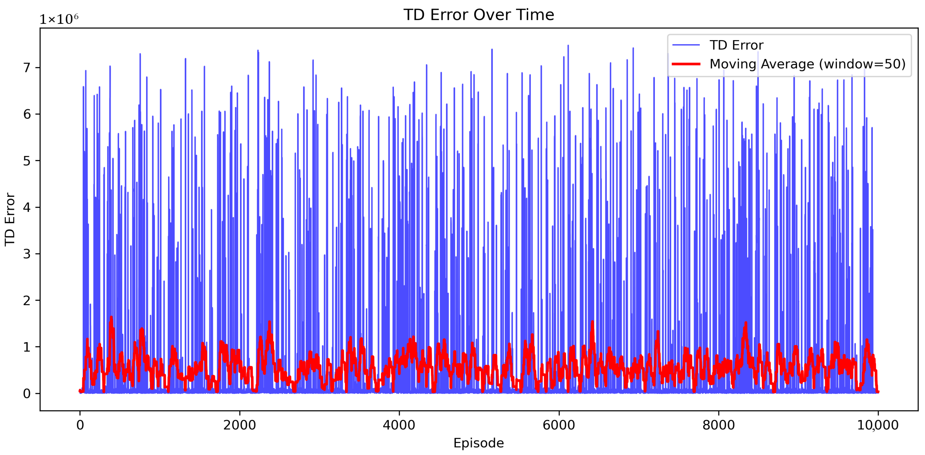
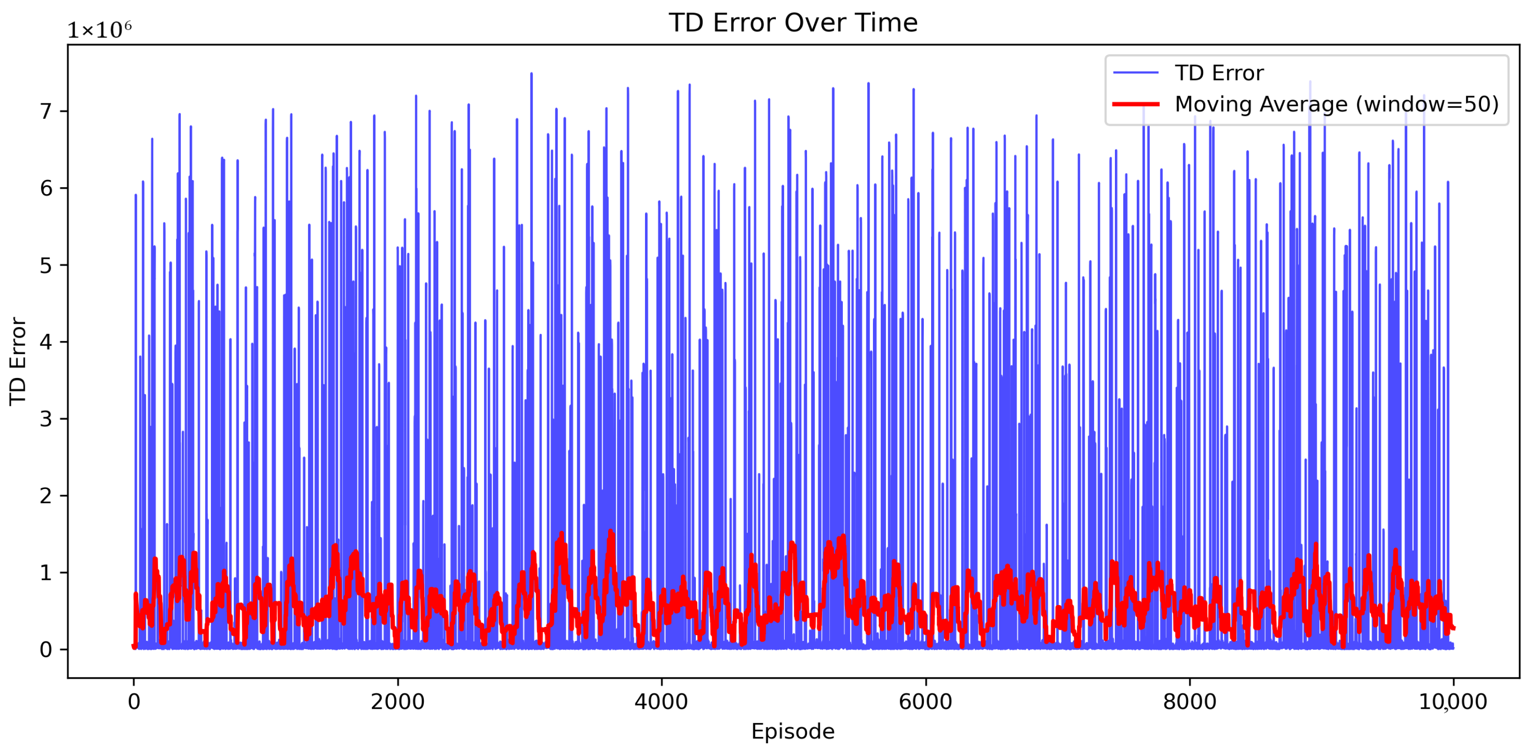
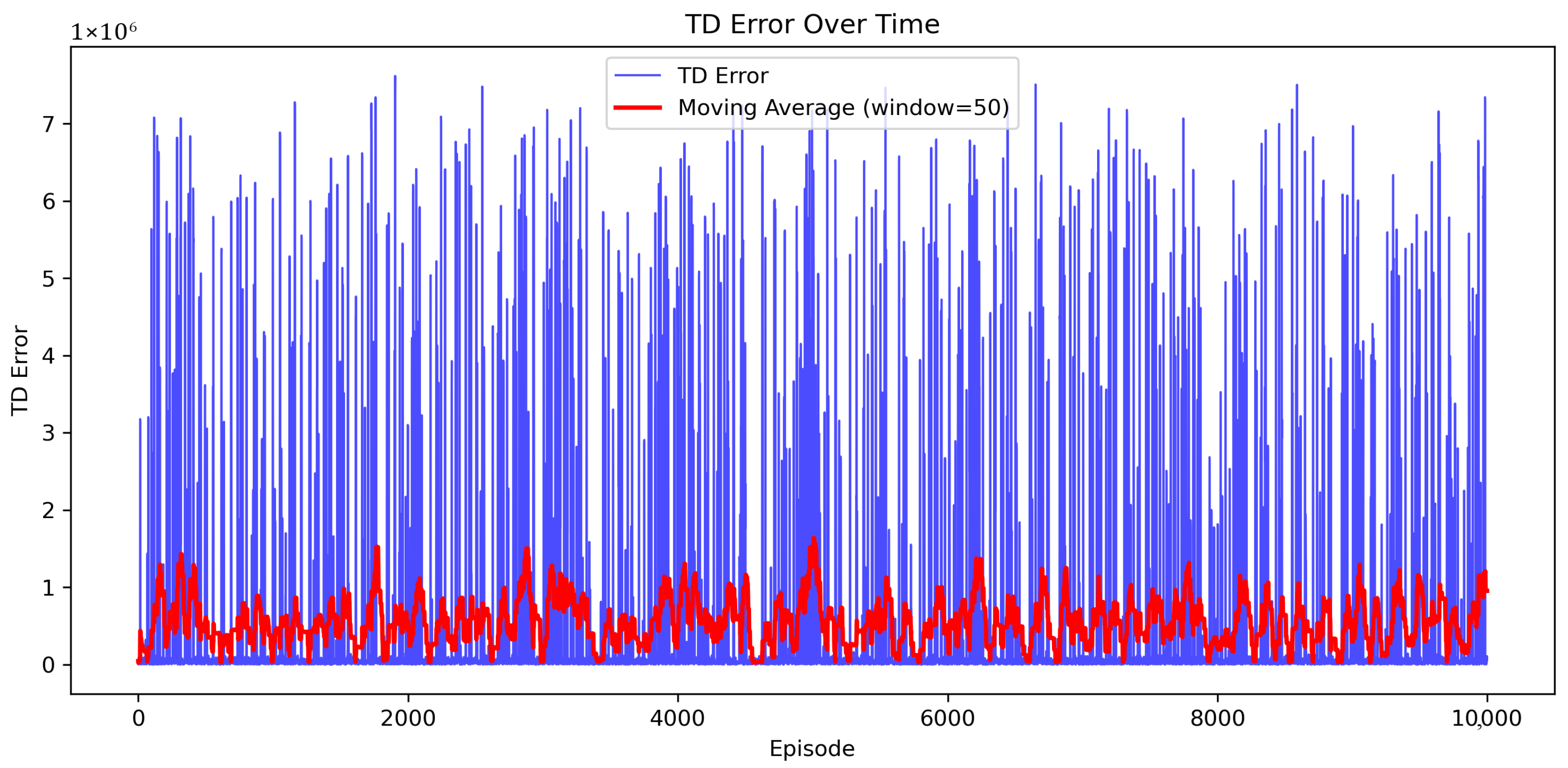
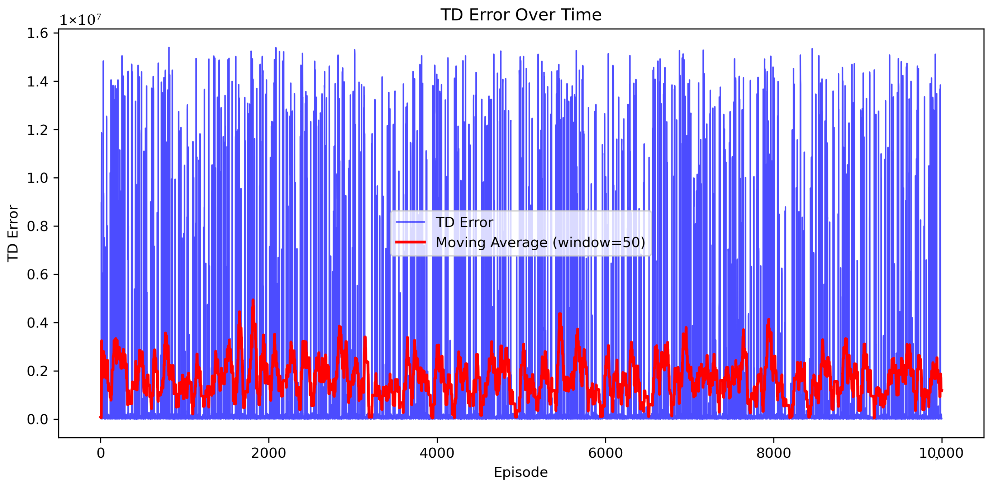
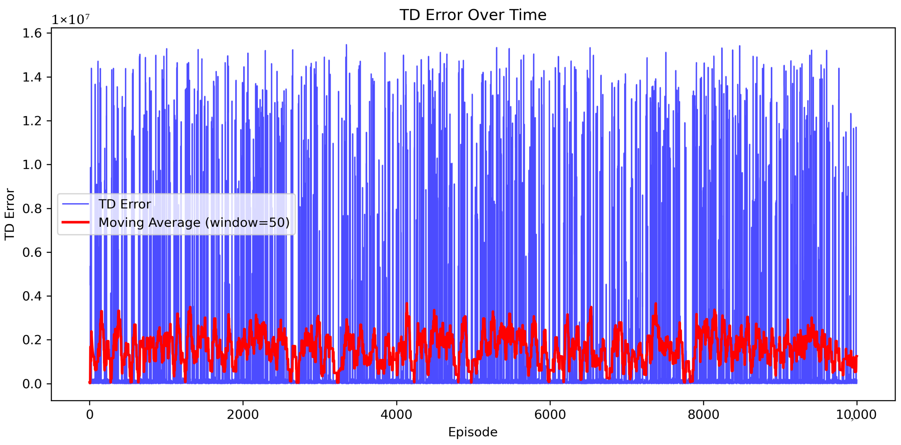
This research aimed to optimize navigation tasks in an urban environment to locate victims. To achieve the research goal, a simulation environment was created, and the UAV, its position, and the LiDAR and infrared camera were simulated. Deep Q-learning algorithms were implemented for the UAV agent, drawing on prior research on navigation tasks in fire environments. The urban environment and the UAV were created using Python’s Pygame library to implement these algorithms. The UAV’s position, LiDAR, and infrared camera were simulated to enable the UAV to collect environmental data. These data streams were fed to the Deep Q-Networks to generate Q-values. Using the Q-value, the TD error was calculated for the Deep Q-networks. Using this TD error, Prioritized Experience Replay (PER) selected the most informative experiences from the buffer for the UAV agent.

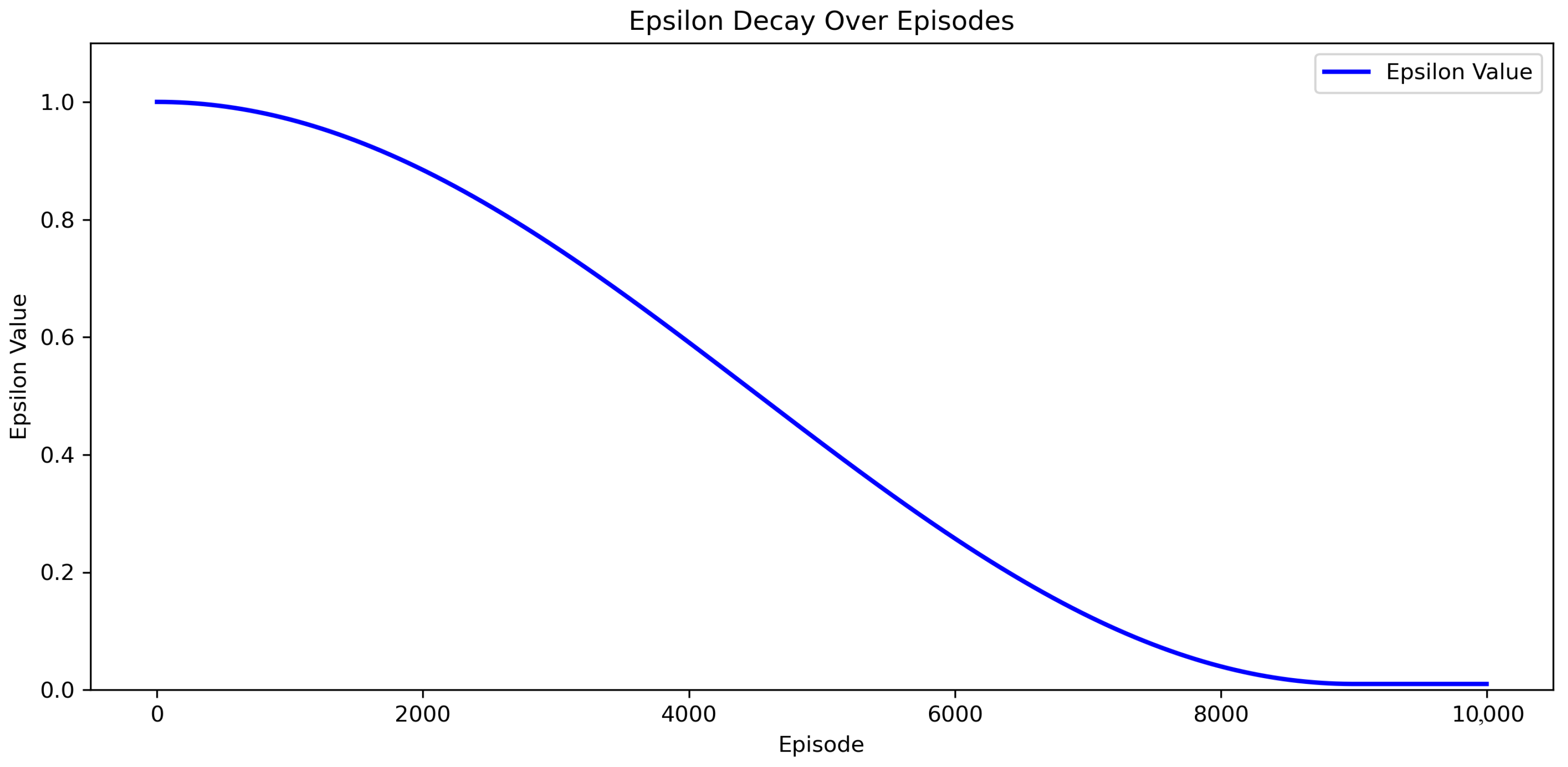
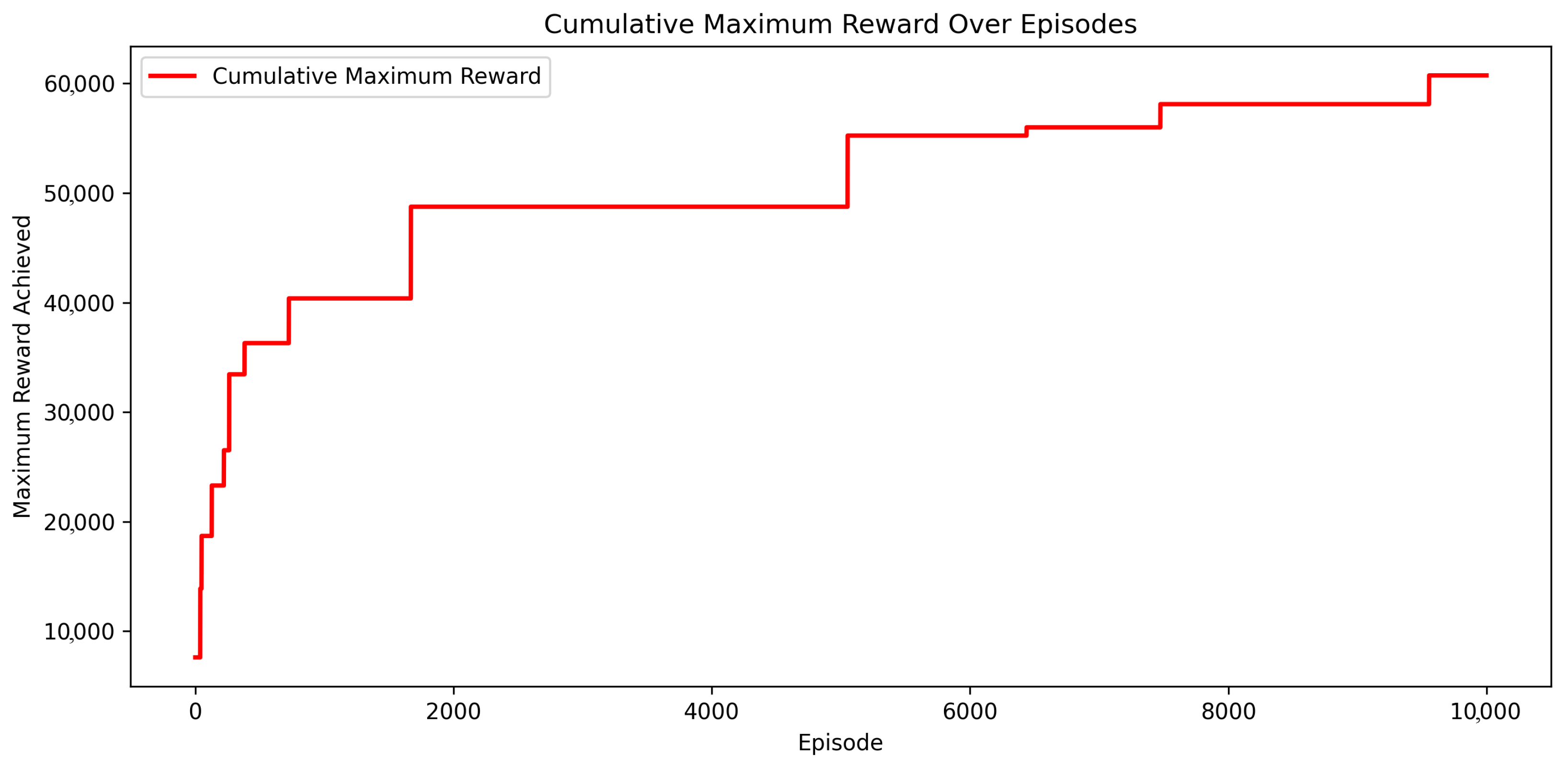
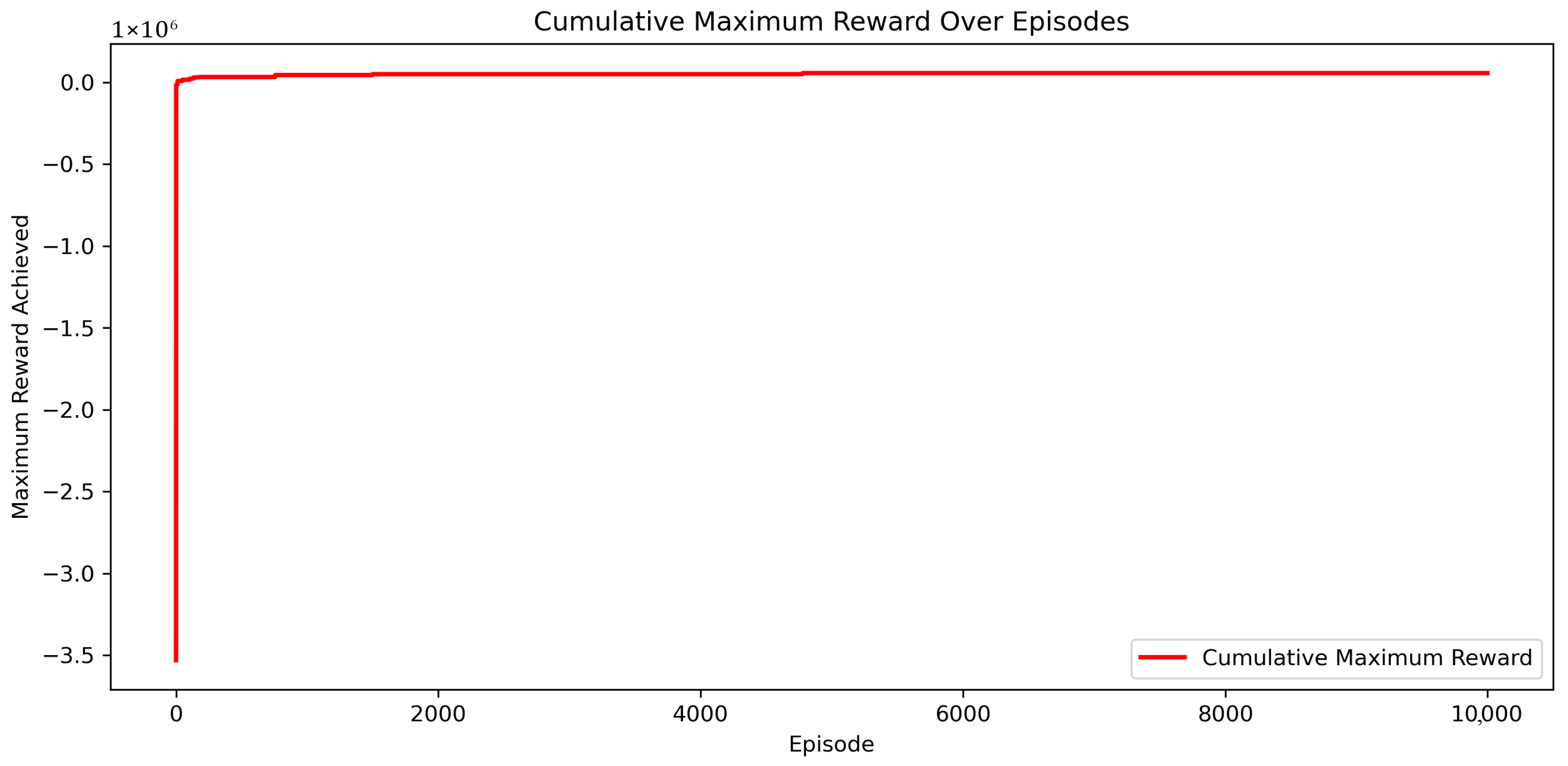
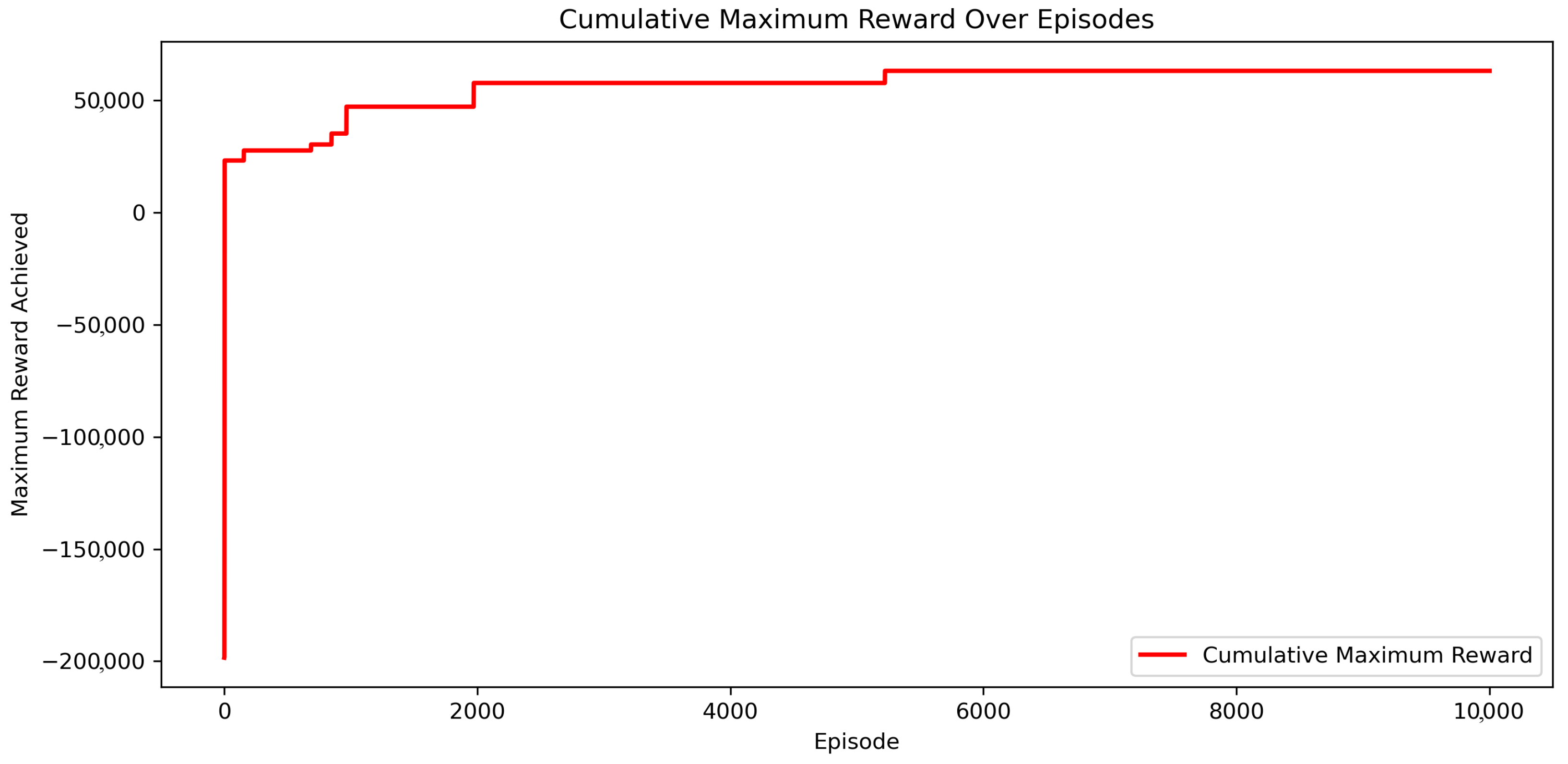
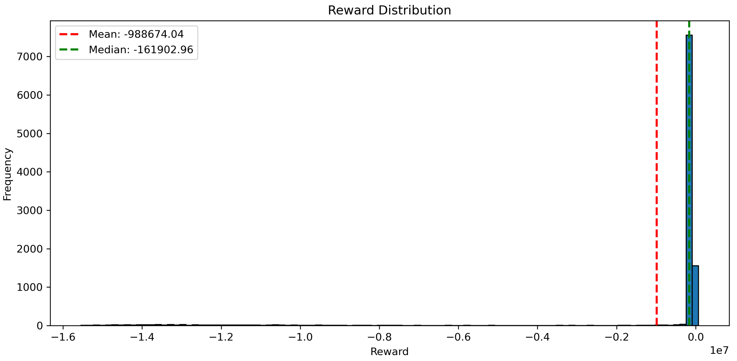
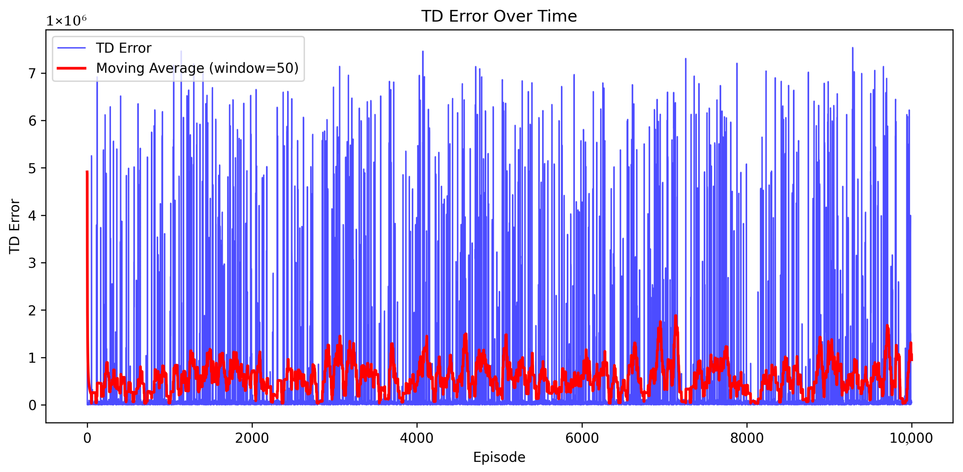
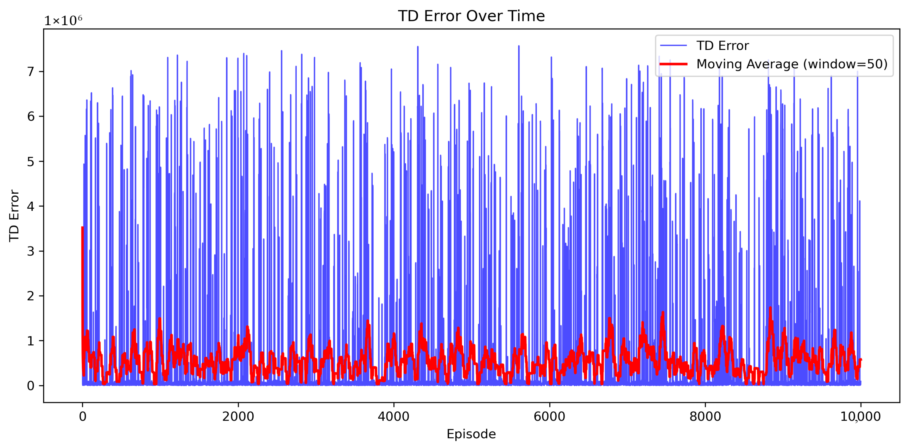
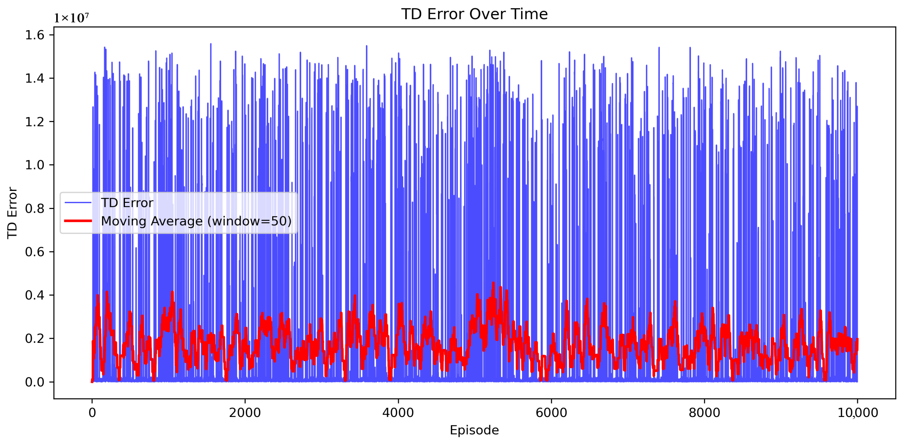
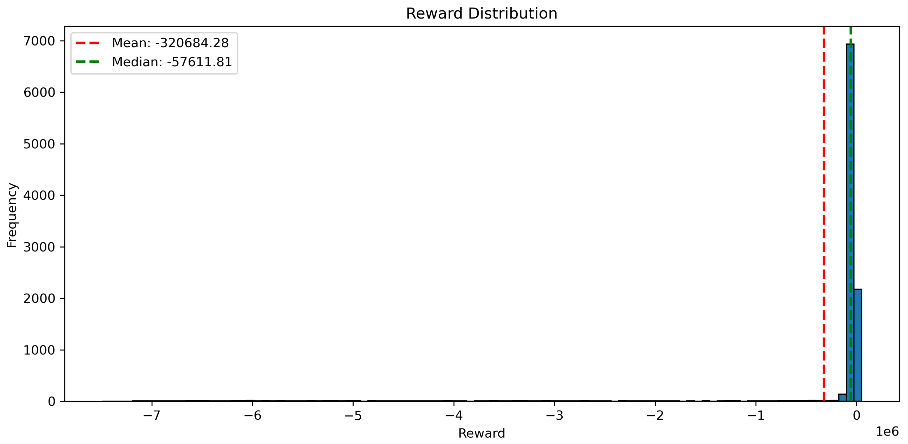
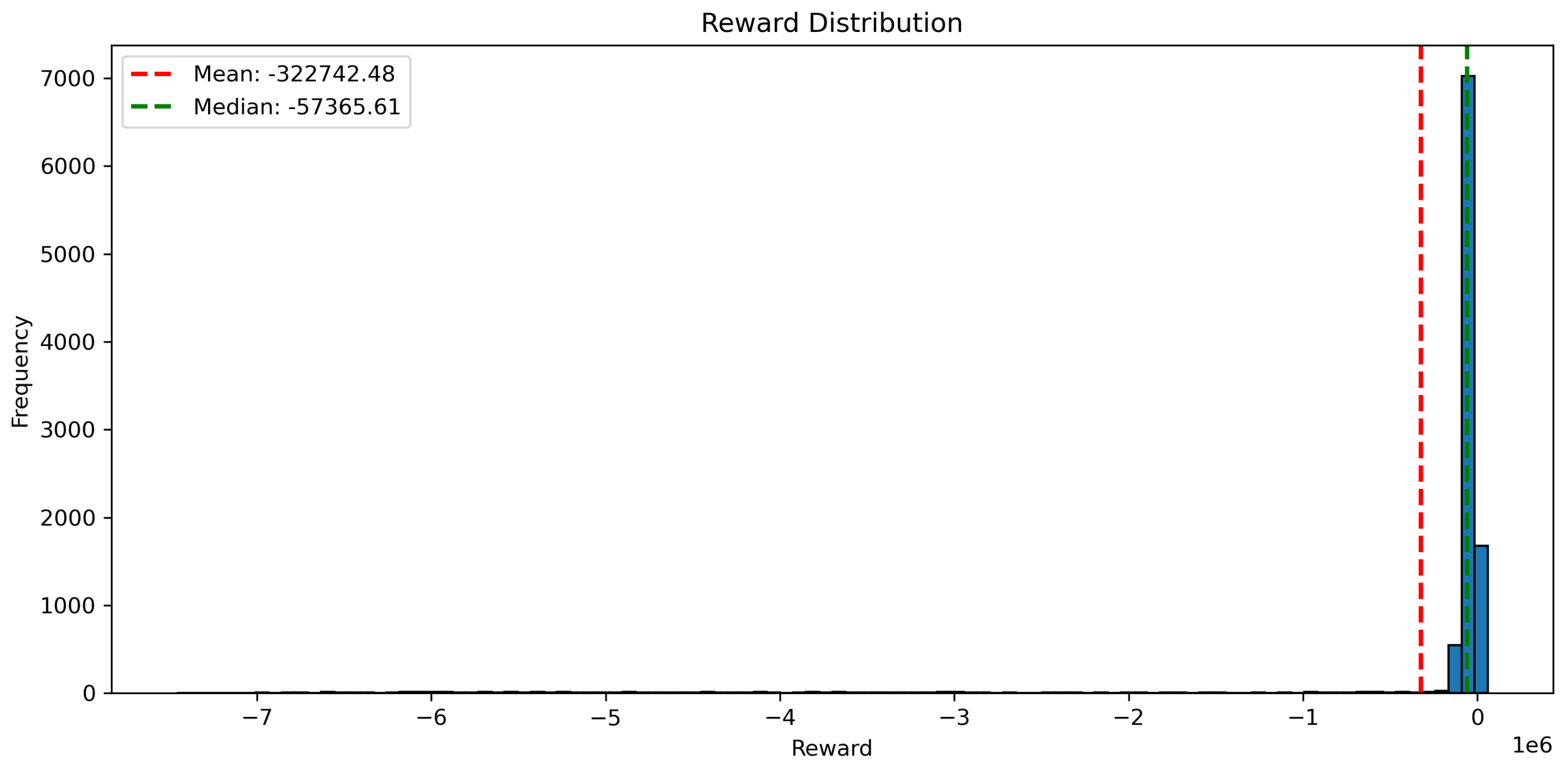
The DQN algorithms were tested over 10,000 episodes. During this training, the exploration rate was varied to maximize the UAV agent’s success. The exploration rate was set to 1.0 at the start of training, allowing the UAV agent to make random moves and learn a rewarding strategy. The exploration rate gradually decreased, allowing the UAV agent to apply the strategy it had learned at the beginning of training. This exploration-exploitation technique is essential for the UAV agent’s success. Parallel processing was employed to accelerate the training. The models were optimized to run on both CPU and GPU partitions of Texas State University’s LEAP2 supercomputer. Each model required 240 gigabytes of memory. The runtime for the models used in this research was typically one to three and a half days.

The reward function for the DQN agents in this research was carefully tuned and developed to account for all parameters of the simulated environment and the UAV agent. The reward function includes basic navigation rewards for completing checkpoints in the proper sequence, a progress bonus for the UAV agent, wall-following rewards, penalties for undesirable behaviors, and distance-based rewards for specific behaviors. The reward function is a crucial component of the simulation and must be sufficiently complex for the DQN agents to succeed.

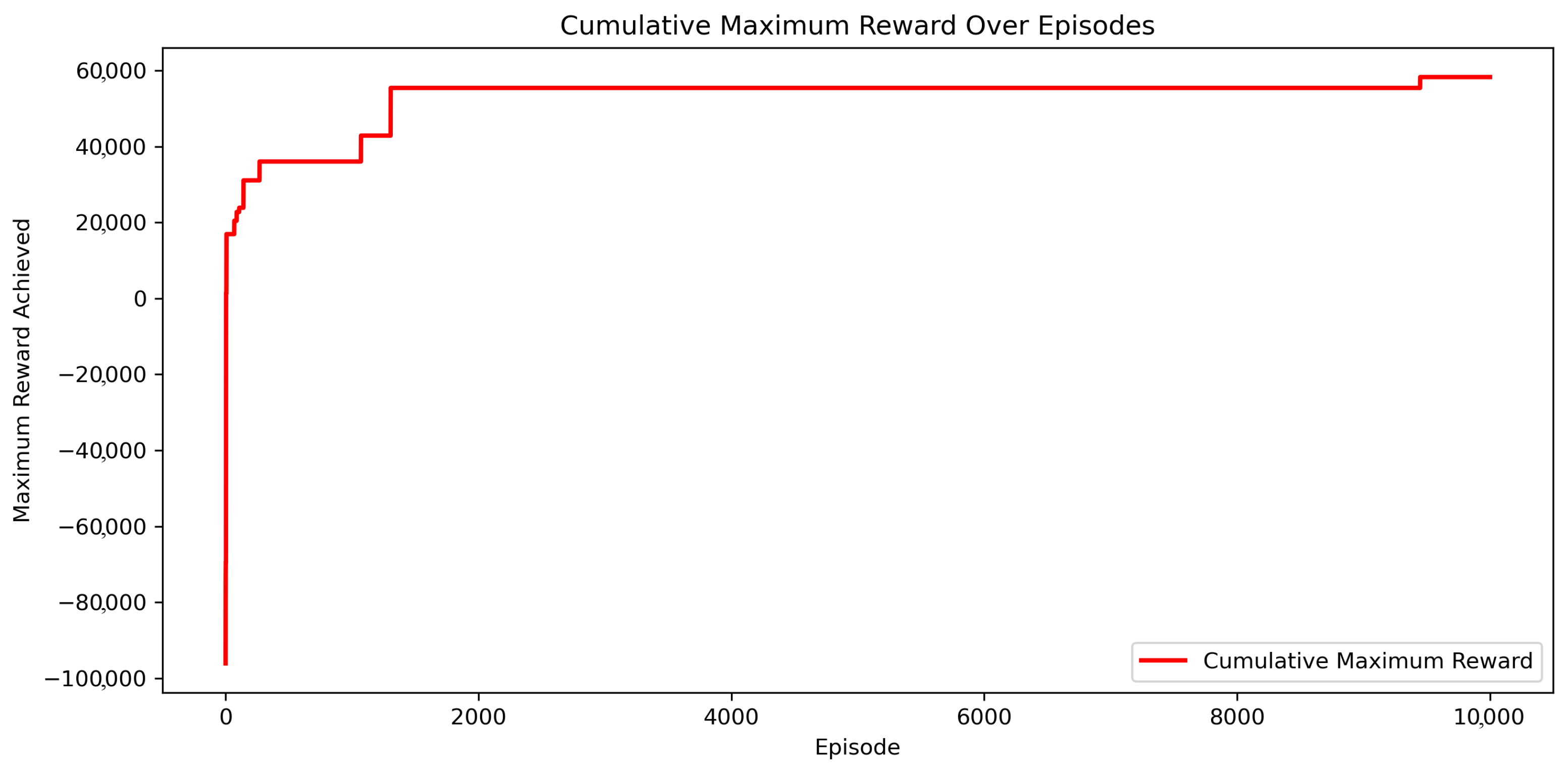
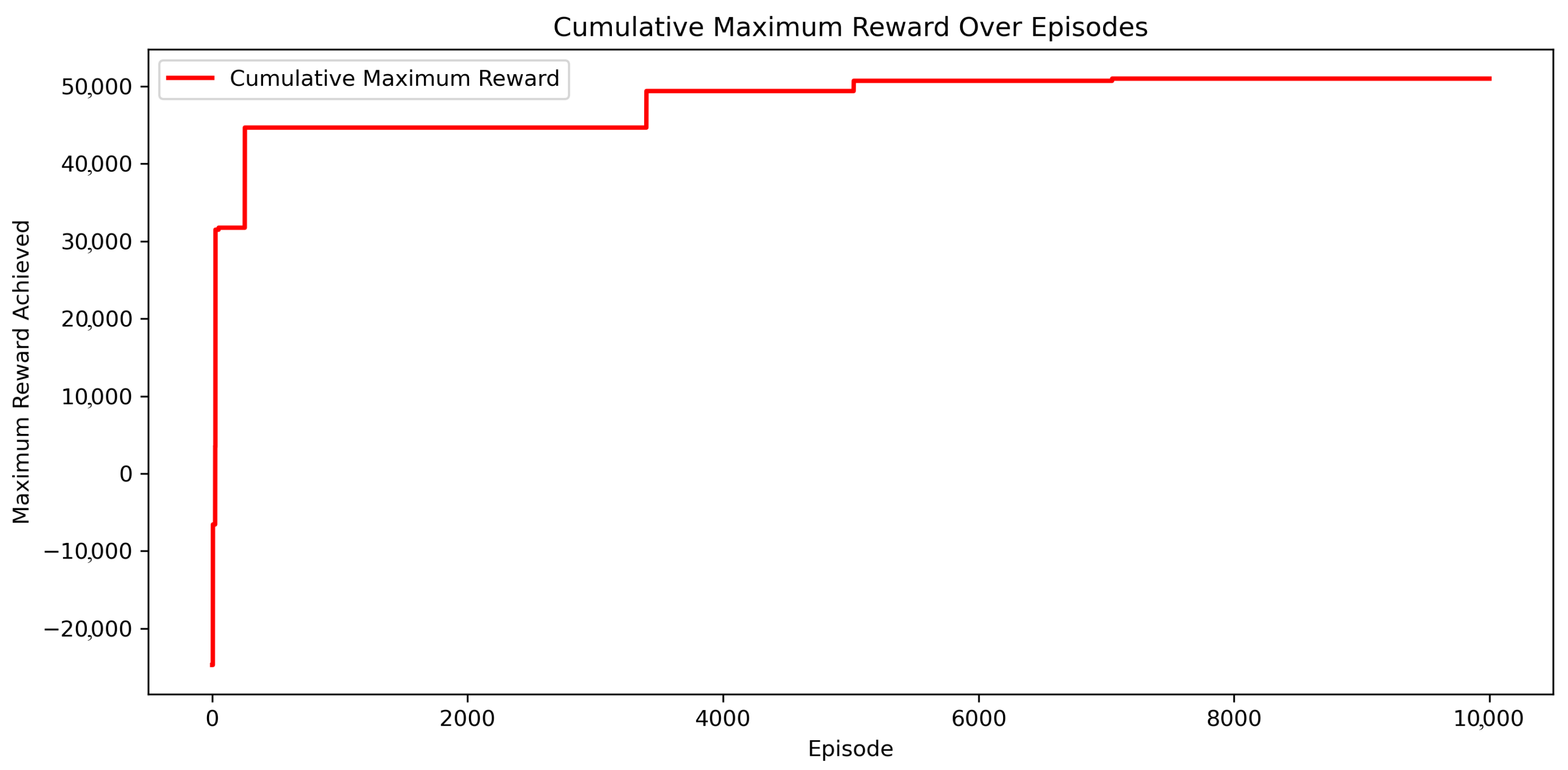
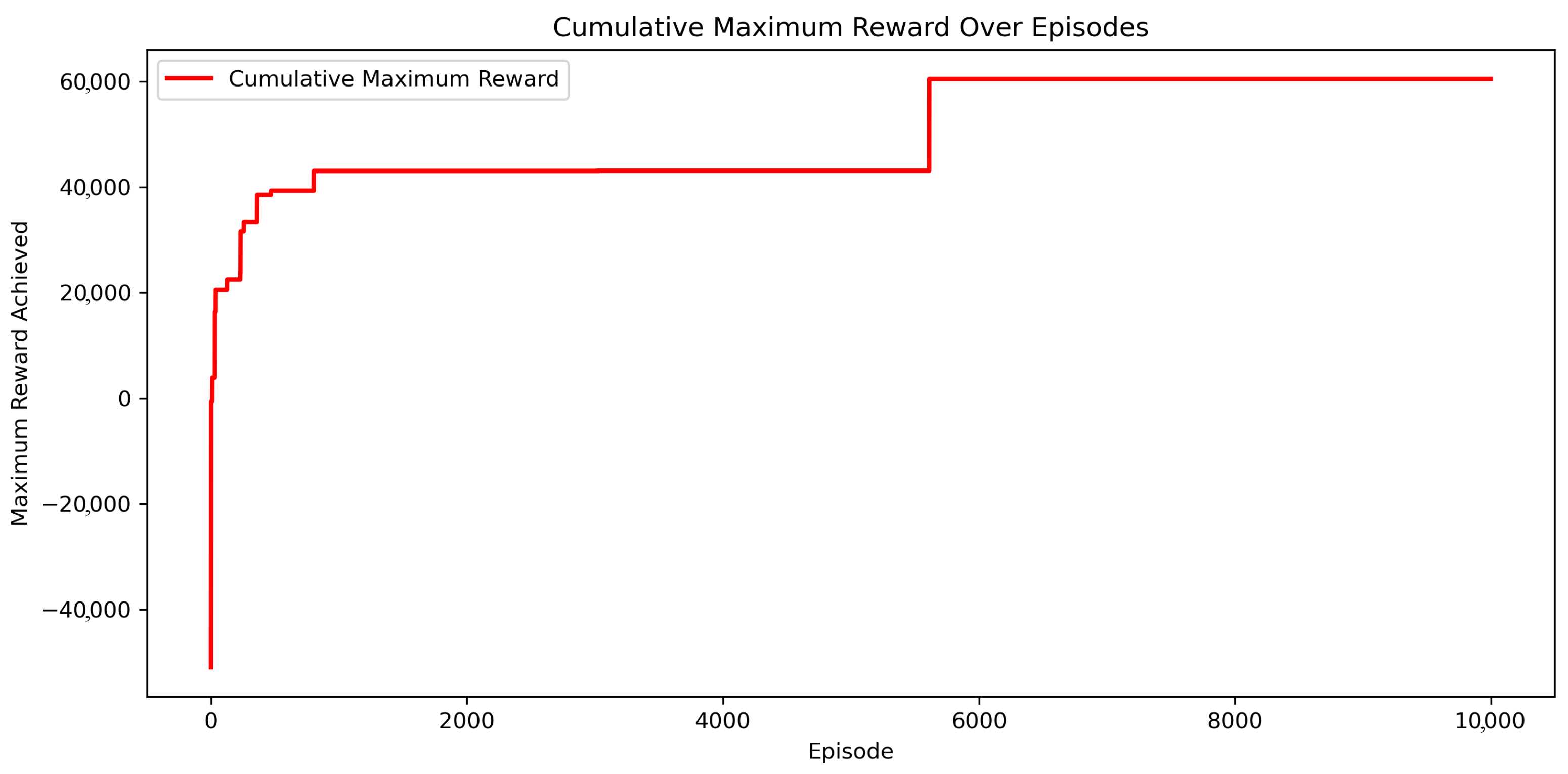
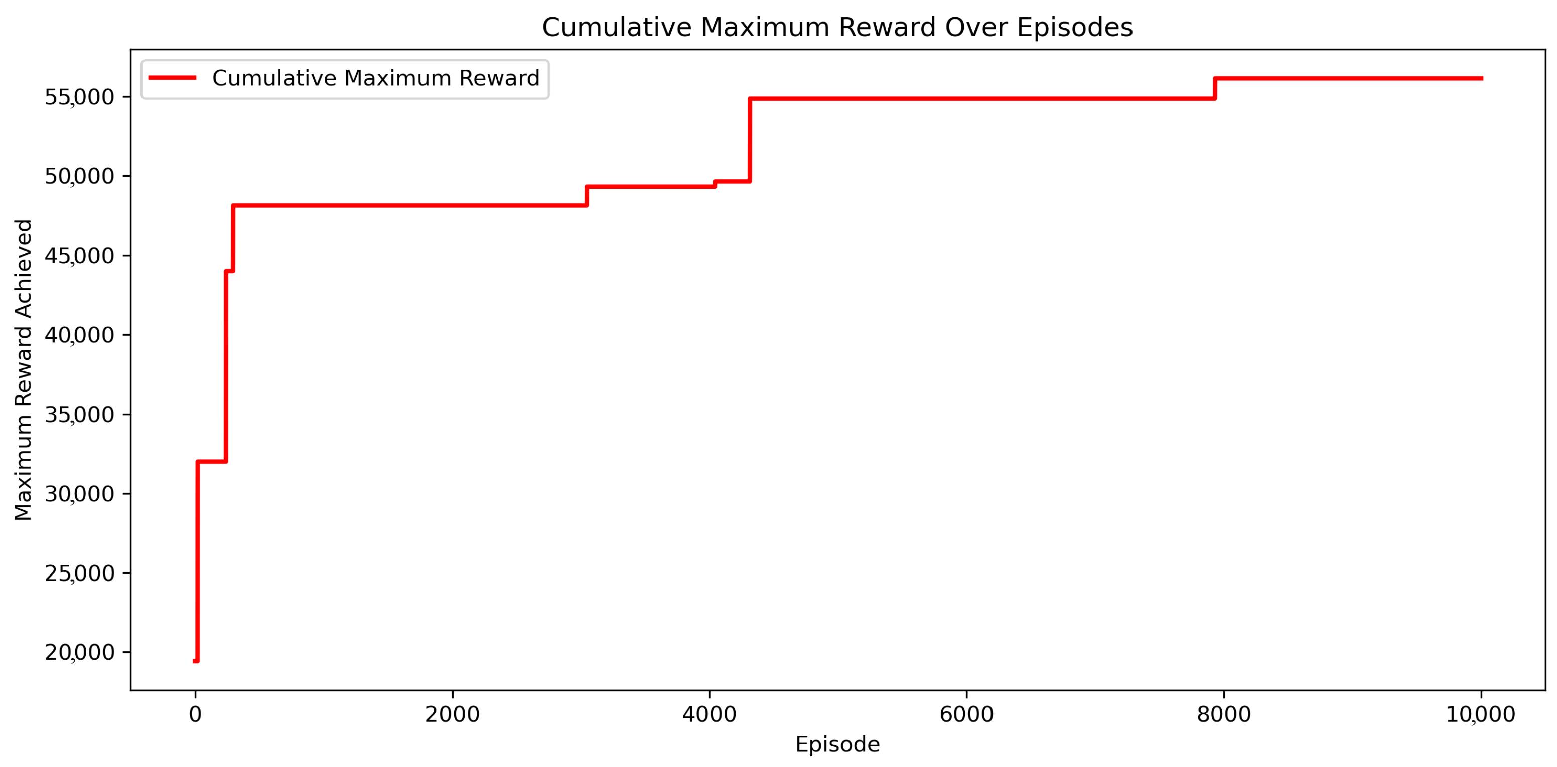
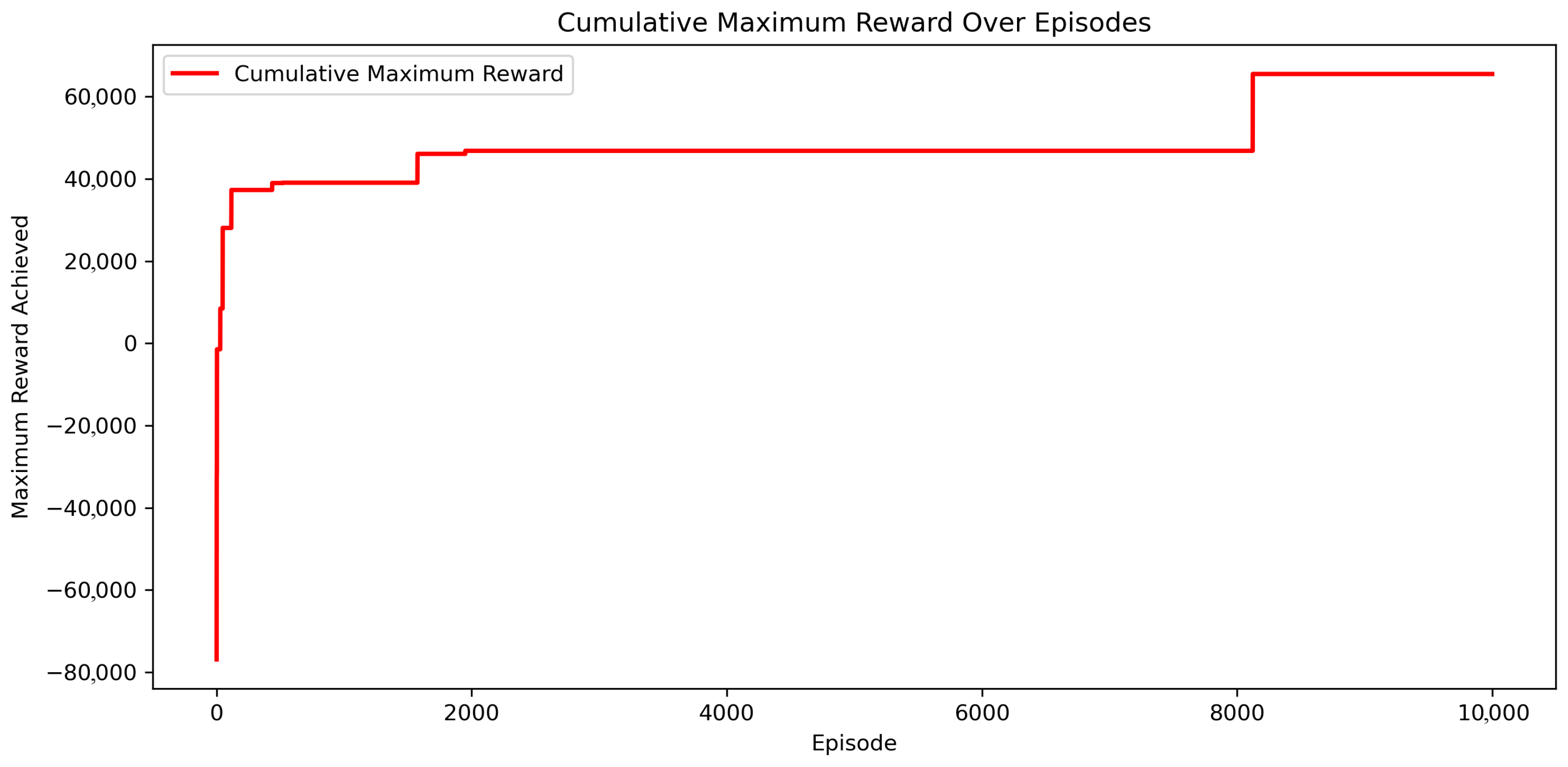
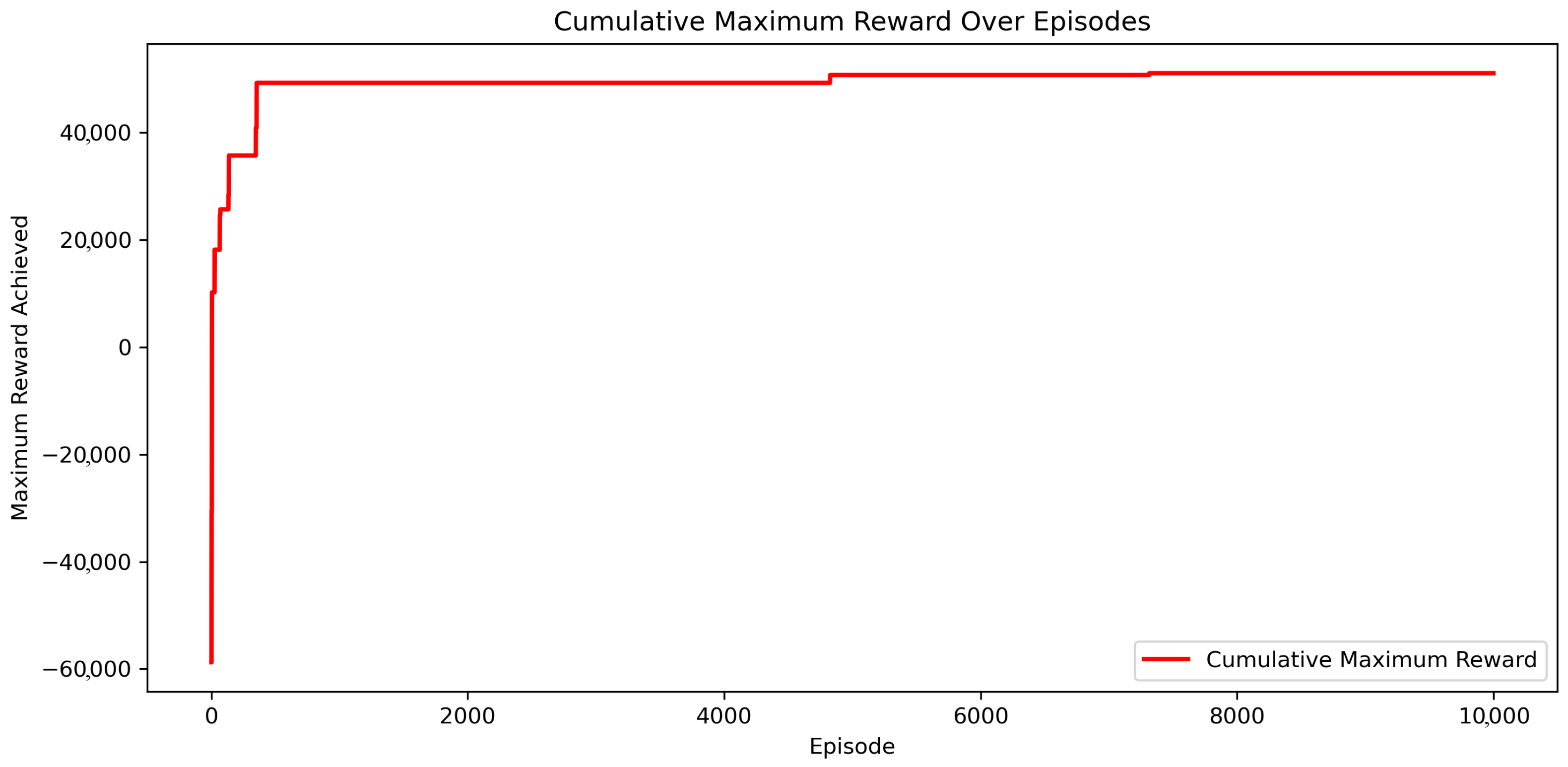
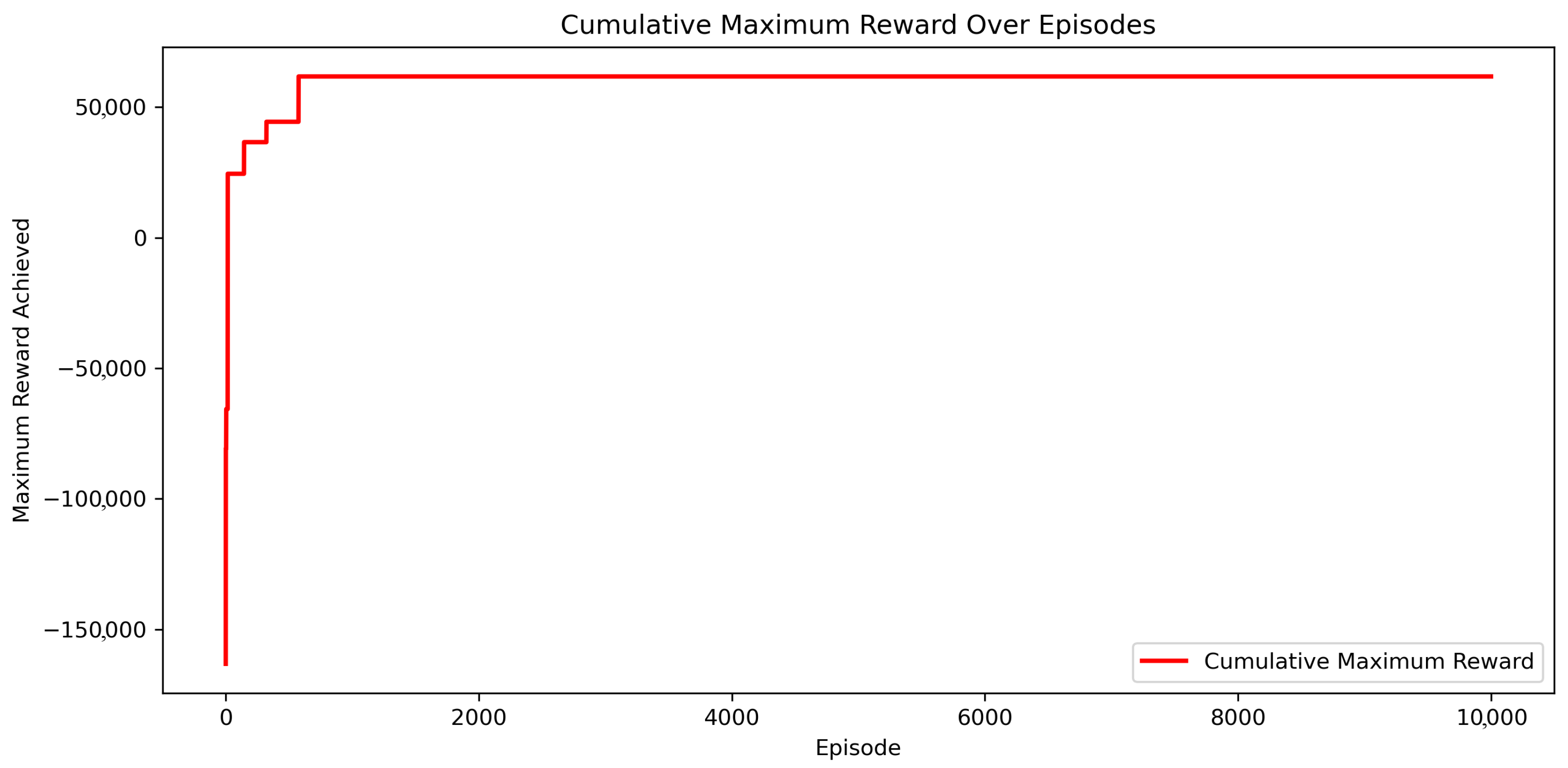
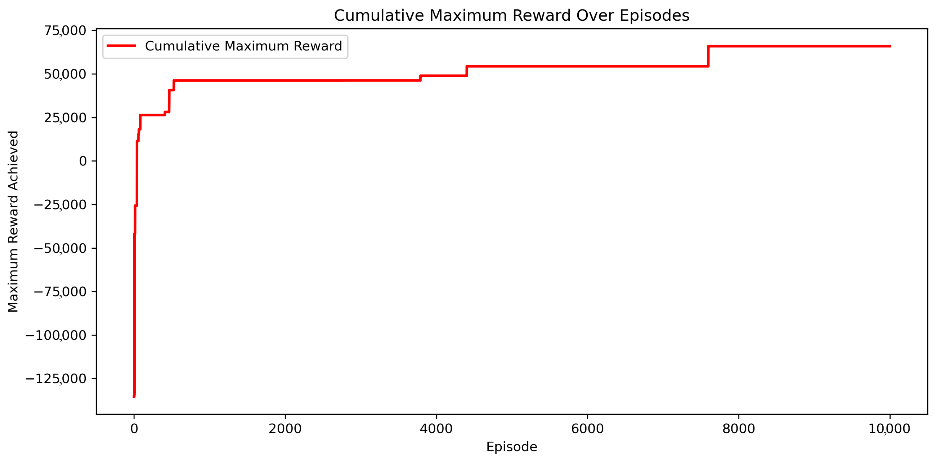
Among the three algorithms, the Double DQN and Dueling DQN performed best in this study. The Double DQN algorithm completed the highest number of episodes successfully in 4000-step limit conditions, and the Dueling DQN algorithm completed the highest number of episodes successfully in 8000-step limit conditions. The Double DQN achieved the highest number of successful episodes, at 128. The Double DQN performed well under 4000-step limits for both single-process and multi-process training. The Dueling DQN achieved 126 successful episodes within an 8000-step limit for the single-process model. For the remaining models, the Dueling DQN performed moderately. The D3QN model performed moderately under the 4000-step and 8000-step limit-condition models, using the single-process model. The D3QN performed worst for the 8000-step limit multi-process model. The D3QN algorithm was slow to learn effective policies and achieved the fewest successful episodes among the three DQN algorithms. In the 8000-step limit multi-process condition, the D3QN algorithm took too long to reach an effective policy for a successful episode.

This research laid the groundwork for navigation and victim detection in complex urban fire environments. The future of this research lies in simulating multiple rooms in a house within urban fire environments, incorporating both external and internal obstacles. When simulating more complex environments, computational resource requirements must be taken into account. The memory usage to run each model for this research was 240 gigabytes. For more complex environments, more than 240 gigabytes of memory may be required. These DQN algorithms can be applied to a physical drone to assist with urban fire rescue operations. Before implementing the DQN algorithms on the physical UAV, the UAV agents must be simulated in a realistic physics environment. Various popular physics simulators are available today, including Gazebo and Unity. These can be used to create multi-room complexes with multiple windows, as well as multi-elevation urban environments with multiple victims. In addition, these physics simulators can be used to model realistic environmental conditions, including fire, wind, and smoke. These physics simulators can also accurately simulate LiDAR and infrared cameras in 3D environments and integrate nicely with the Robot Operating System (ROS). With accurate simulation of the burning structure, multi-agent DQN algorithms can be used to navigate around it at different elevations to locate victims on different floors. This research is currently limited to the resources available at Texas State University’s High-Performance Engineering Laboratory. When more resources are available, the multi-agent, multi-room, realistic environments will be simulated using physics simulators.

6. Conclusions

This research investigates the potential of utilizing Double DQN, Dueling DQN, and D3QN to aid firefighters in locating victims in urban environments. To utilize DQNs in this work, a UAV equipped with position, LiDAR, and infrared camera data was simulated, and a complex environment was created using Python’s Pygame library. Data from the UAV’s sensors were fed to the DQNs, and UAV actions were selected based on the reward function.

The results of this research indicate that the UAV agents completed the goals set by the reward function. The Double DQN and Dueling DQN performed well compared to D3QN. This research presents a simulation-based proof-of-concept demonstrating that the Double DQN and Dueling DQN can be applied in real-world scenarios. These neural networks can be used for navigation around a burning structure at multiple elevations, employing multiple UAVs to search for victims. The use of multiple UAVs for navigation tasks in urban environments will significantly reduce the effort and time firefighters spend searching for victims.

Validating the results of this research by integrating DQNs into a UAV in real-world urban firefighting scenarios will significantly impact urban firefighting scenarios. Future work for this research involves integrating and testing the DQNs in real-world scenarios. To achieve this, physics and environmental factors will be considered. This work lays the groundwork for integrating DQNs into UAVs for navigation and victim detection in urban environments. Several physics simulators are available today and will be used in future work to simulate and validate the effectiveness of DQNs in the real world.

This research advances the emerging field of firefighting robotics by employing DQNs to enable autonomous navigation. It compares the effectiveness of navigation tasks in a fire environment across the Double DQN, Dueling DQN, and D3QN, paving the way for real-world UAV applications in firefighting. The results of this study provide insights into how DQNs can be used for navigation tasks in urban environments for firefighting, as well as their potential applications in various fields, including locating victims in disaster scenarios.