Determining Fault Locations on Overhead Power Lines Under Power Quality Deviation Conditions Based on the Least Squares Method

Abstract

Overhead power lines (OHPLs) are currently widely used to generate power from various types of traditional power plants and transmit power between electric power systems (EPSs). OHPLs are known to be susceptible to climatic, meteorological, man-made, and other factors, which leads to more frequent outages with damage of varying severity. Ensuring reliable operation of the EPS requires rapid and accurate fault location (FL) for emergency restoration operations and the subsequent restoration of the OHPL. This article presents the results of an analysis of various methods for FL of OHPLs under conditions of deviations in power quality indicators (PQI), which leads to additional FL errors in emergency mode parameters (EMP). The objective of the study is to develop a new method for FL on OHPLs with unsynchronized measurements from both ends under conditions of current and voltage deviations from a sinusoidal shape, based on the least-squares method. The developed method for FL on OHPLs is based on differential equations describing the currents and voltages in emergency conditions at both ends, taking into account distributed transverse (capacitive) conductivity. This significantly improves the accuracy of FL on OHPLs with unsynchronized measurements at both ends under conditions of fluctuating power quality parameters. The article presents calculation results for a specific OHPL, demonstrating the improved accuracy of FL based on the EMP. The developed method can be implemented in digital protection and automation devices for OHPLs, as well as in software for power system control centers.

1. Introduction

In modern electric power systems, overhead power lines (OHPLs) of various voltage classes remain the cheapest and most efficient means of transmitting electricity. In the EPS of most countries, there are many OHPLs; they have a greater total length compared to cable power lines [1,2].

The lower reliability of OHPLs is due to their exposure to various climatic, meteorological, man-made, and other factors [3,4,5]. According to statistics, the primary faults on OHPLs 110 kV and above are single-phase short circuits (SCs), accounting for up to 70% of all faults. Two-phase and three-phase SCs account for 20% and 10% of faults, respectively [6]. To improve the reliability of the EPS, some countries are implementing programs to convert OHPLs to cable-based systems. However, this solution is quite expensive and requires significant capital investment [7,8].

High-voltage, extra-high-voltage, and ultra-high-voltage OHPLs are widely used to generate power from various types of conventional power plants, as well as to transmit power between regional power systems [9,10]. In the last decade, DC power lines have become widely used alongside AC power lines. However, they are not considered in this study, as their FL methods are fundamentally different.

SCs on OHPLs cause voltage dips. The depth and duration of these dips depend on several factors: the type of SC, the contact resistance at the FL, the settings and operating logic of protection devices, and the tripping time of high-voltage circuit breakers [11]. Such voltage dips negatively affect electrical equipment, particularly electric motors [12,13]. This is because motors brake during the SC and then must self-start once it is cleared [14,15].

In some cases, OHPLs with voltages of 110 kV and higher pass through mountainous, forested, and marshy areas, crossing streams, rivers, lakes, and artificial reservoirs. The length of such OHPLs can be hundreds of kilometers, significantly complicating both FL and emergency recovery operations [16]. Rapid and accurate FL detection on OHPLs is a pressing issue, as it ensures the reliable operation of the EPS.

The widespread introduction of power electronics into EPS leads, under certain conditions, to deviations in power quality indicators (PQIs) from standard values [17,18]. Power electronics are widely used in renewable energy power plants, in various power system control devices, such as FACTS, and in industrial power supply systems, such as soft starters, variable frequency drives, and other devices [19]. When PQI deviates from standard values, installed FL devices can produce significant errors, leading to increased time spent locating and repairing the fault. As a result, the operational reliability of the power system will be reduced, which is highly undesirable [20,21,22].

Despite the extensive research on FL detection on OHPLs [23,24,25,26,27,28], the development of reliable and accurate algorithms for calculating the distance to the FL remains a complex task. Recent publications on the results of SC tests at main power grid facilities indicate low errors and the potential for using traveling wave FL detection on OHPLs [29,30,31,32], including those based on active probing methods for OHPLs [33,34]. However, the use of FL detection algorithms on OHPLs based on emergency mode parameters (EMP) remains relevant, given the availability of information on current and voltage parameters in digital protection and automation devices [35,36,37,38].

Errors in FL of OHPLs stem from several factors. These include the use of simplified power system models when developing FL algorithms, inaccuracies in specifying power system characteristics (such as complex EMF, source resistances, and longitudinal and transverse specific complex impedances of power lines), unknown SC resistance, the influence of load parameters, and mutual coupling with adjacent lines on shared corridors [39,40,41]. A random combination of these factors significantly affects the accuracy of FL analysis. Additional errors are introduced by deviations in electrical PQIs [42].

Errors in FL on OHPLs can be reduced in two main ways. One is by refining data on power system parameters. The other is by using special mathematical methods for information processing, such as artificial intelligence [43,44,45]. The use of new digital signal processing methods is especially valuable. This is particularly true when calculations rely on instantaneous current and voltage values from oscillograms recorded during emergency conditions on OHPLs [46,47].

The aim of this study is to develop a new method for FL on OHPLs using unsynchronized measurements from both ends under conditions where PQIs (currents and voltages from a sinusoidal shape) deviate from standard values, based on the least-squares method (LSM). The FL method is implemented using differential equations describing the fault currents and voltages recorded at the ends of the power line, taking into account distributed transverse (capacitive) conductivity.

The article is structured as follows. Section 2 examines methodological issues related to using different models for FL on OHPLs. It also explains why transverse (capacitive) conductivity should be taken into account when PQIs deviate from standard values. A calculation example shows that when PQIs such as flicker and interharmonics deviate, known FL methods based on EMPs produce significant errors in calculating the distance to the fault. Section 3 presents a newly developed FL method. This method accounts for distributed transverse (capacitive) conductivity and uses the LSM to calculate the FL when PQIs deviate. Section 4 demonstrates that the new method provides high accuracy in calculating the distance to the fault even when PQIs deviate. This accuracy meets operational requirements. The paper also explores the feasibility of implementing this new method using unsynchronized measurements of emergency currents and voltages from both ends. Section 5 presents the main conclusions of the article.

2. Materials and Methods

When locating faults on OHPLs, high accuracy is essential for rapid FL and emergency restoration operations [48]. To ensure high-precision FL on OHPLs, it is necessary to consider the need for transverse (capacitive) conductivity. In the present study, the data source consists of current signals corrupted by flicker, simulated in MathCad 15 (Mathsoft, Cambridge, MA, USA) with a sampling interval of t_d = 0.0025 s. It should be noted that the simulation was conducted under idealized current measurement conditions. When assessing the potential of the FL method, the error of current transformers (CTs) was not taken into account, as it could blur the accuracy characteristics of the method itself.

2.1. Analysis of the Influence of Capacitive Conductivity

In [49], it is noted that a preliminary assessment of the need to take into account transverse (capacitive) conductivity should be carried out. Neglecting transverse conductivity (especially when performing manual FL calculations) is permissible if the resulting error in calculating the distance to the fault does not exceed 2%. The error from neglecting transverse conductivity depends on the length of the OHPL and the resistance of the adjacent electrical network.

On this issue, the following recommendations are given in [49]. When using zero-sequence parameters to calculate the FL on OHPLs, it is permissible to neglect the transverse (capacitive) conductivity for OHPLs up to 100 km long, and when using negative-sequence parameters—up to 120–150 km. For OHPLs of greater length, for which the ratio of the resistances of the adjacent electrical network and the power line in question is of primary importance, it is permissible to ignore the transverse conductivity for OHPLs up to 200–250 km long if this ratio is in the range of 0.1–0.5.

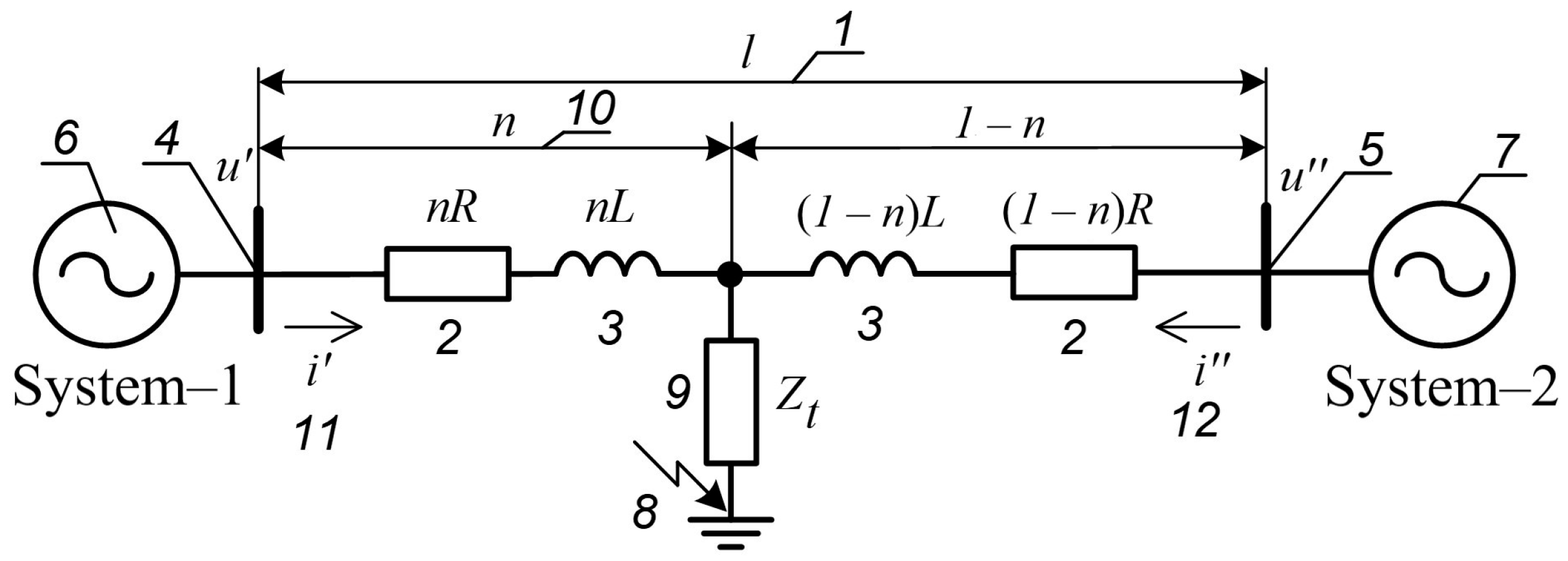
A single-line equivalent circuit diagram of an OHPL that does not take into account its transverse (capacitive) conductivity is shown in Figure 1. The following designations are introduced in Figure 1: 1—length of the OHPL (l); 2—phase active resistance (R); 3—phase inductance (L); 4 and 5—buses of two power systems; 6 and 7—power systems. On the OHPL, an SC—8 is shown behind the transition impedance (Z_t)—9 at a distance n—10 from one end of the OHPL. When a short circuit occurs on an OHPL, a current (i′) flows through it from bus 4 and a current (i″) from bus 5. In this case, the instantaneous values of phase currents (i′_A, i′_B, i′_C), (i″_A, i″_B, i″_C) and voltages (u′_A, u′_B, u′_C), (u″_A, u″_B, u″_C) at the moment of the SC are measured on buses 4 and 5 at both ends of the OHPL, not synchronized in time.

Using the differential equation for OHPLs [50,51] allows us to calculate the relative distance to the FL n in accordance with expression (1):

$$n ={\displaystyle \frac{\left(u^{\prime }\left(m\right) - u^{″}\left(m\right)\right)+ R·i^{″}\left(m\right) + L·\frac{i^{″}\left(m\right)}{{dt}_m}}{R·\left(i^{\prime }\left(m\right) + i^{″}\left(m\right)\right) + L·\left(\frac{i^{\prime }\left(m\right)}{{dt}_m} + \frac{i^{″}\left(m\right)}{{dt}_m}\right)}}.$$

(1)

This method for determining the FL on OHPL has small errors when calculating the distance to the FL during an SC with undistorted (sinusoidal) currents and voltages in the oscillograms of the emergency mode [50].

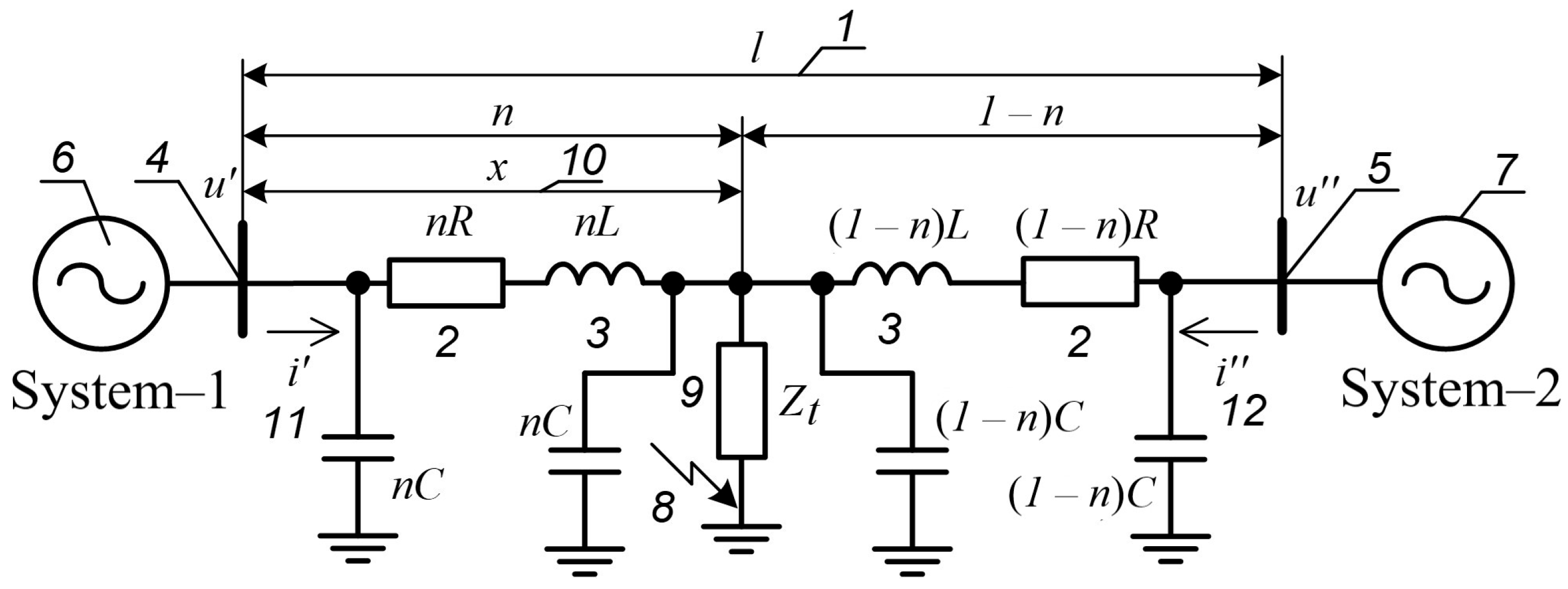
When taking into account transverse (capacitive) conductivity, the equivalent circuit for determining the FL on OHPL changes and takes the form shown in Figure 2. In the equivalent circuit (Figure 2), compared to Figure 1, the elements of distributed transverse (capacitive) conductivity are indicated—11 and 12.

The differential equations describing the relationship between currents and voltages on the faulted OHPL will change accordingly. In this case, the voltage drops to the SC point at both ends of the OHPL (Figure 2) can be determined using expression (2):

$$\begin{gathered} \hspace{1em}\hspace{1em}{u}^{\prime }-n·i^{\prime }·R-n·L·{\displaystyle \frac{d{i}^{\prime }}{dt}}+n·R·C·{\displaystyle \frac{d{u}^{\prime }}{dt}}+n·L·C·{\displaystyle \frac{d^2{u}^{\prime }}{{dt}^2}}=U= \\ =u^{″}-\left(1-n\right)·i^{″}·R-\left(1-n\right)·L·{\displaystyle \frac{d{i}^{″}}{dt}}-\left(1-n\right)·R·C·{\displaystyle \frac{d{u}^{″}}{dt}}+ \\ \hspace{1em}+\left(1-n\right)·L·C·{\displaystyle \frac{d^2{u}^{″}}{{dt}^2}} , \end{gathered}$$

(2)

where L and C are the longitudinal inductance and transverse capacitance of the OHPL, corresponding to the equivalent circuit in Figure 2.

After transforming expression (2), we obtain expression (3) for calculating the distance to the FL on OHPL in the diagram in Figure 2:

$$n = {\displaystyle \frac{\left(u^{\prime }- u^{″}\right) + i^{″}· R + L·\frac{d{i}^{″}}{dt} - R·C·\frac{d{u}^{″}}{dt} - L·C·\frac{d^2{u}^{″}}{{dt}^2}}{R·(i^{\prime } + i^{″}) + L·(\frac{d{i}^{\prime }}{dt} + \frac{d{i}^{″}}{dt}) - R·C·(\frac{d{u}^{\prime }}{dt} + \frac{d{u}^{″}}{dt}) - L·C·(\frac{d^2{u}^{\prime }}{{dt}^2} + \frac{d^2{u}^{″}}{{dt}^2}) }}.$$

(3)

It is important to note that in expression (3), unlike expression (1), along with the OHPL parameters, voltages u′ and u″, currents i′ and i″, and their derivatives di′/dt, di″/dt, the first du′/dt, du″/dt, as well as the second d²u′/dt², d²u″/dt² derivatives of voltages u′ and u″ are also used. The use of the first and second derivatives of voltage allows us to take into account the transverse (capacitive) conductivity in the equivalent circuit in Figure 2.

Reference [52] notes that using differential equations based on the OHPL model (Figure 2) offers a key advantage. It allows both the aperiodic component and the transient high-frequency components of current and voltage signals to be considered when processing emergency oscillograms. This is done without the need for additional filtering. Accordingly, the FL method using unsynchronized measurements from both ends and the same model (Figure 2) works as follows. It includes transient sources in the algorithm for calculating the distance to the fault (expression (3)). As a result, it does not require filtering transient components from the emergency oscillograms.

Additional causes of FL errors on OHPLs include:

• Deviations in the power system frequency from the nominal value, which cause errors associated with the mismatch of the sampling frequency of current and voltage signals during their digital processing in FL devices [53,54];
• Saturation of current transformers and the corresponding appearance of an aperiodic (constant) component in the sinusoidal oscillograms of emergency currents [55,56,57];
• The presence of multiple harmonics and interharmonics in emergency current and voltage oscillograms, caused, for example, by the influence of industrial electrical consumers [58,59];
• The distorting effect of various interference components in the form of flicker and high-frequency interference [60,61,62];
• Other causes, manifested in the heterogeneity of the OHPLs, the presence of parallel OHPLs and branches, which are not considered in this study.

Since the calculation relationships of the method described in [50] assume that fault voltages and currents are represented by ideal sinusoidal signals with a frequency of f = 50 Hz (without interference), and the calculations are performed using only individual instantaneous values, errors in FL may be significant due to individual deviations in PQIs (or their combined effect). Moreover, deviations in PQIs may be within acceptable limits, and their combined effect on the accuracy of the FL monitoring of an OHPL may be significant.

2.2. Ffirst Calculated Example

To estimate the errors in FL caused by deviations in PQIs, we will use the calculation example given in [50], as well as the calculation expression (1), which includes the instantaneous values of current and voltage at both ends of the OHPL. We assume that i′(m) and di′(m)/dt_m, as well as i″(m) and di″(m)/dt_m are quadrature (orthogonal) components obtained at a certain point in time (m). Then the current amplitudes at the ends of the OHPL can be determined using expressions (4):

$$I^{\prime }=\sqrt{{\left[i^{\prime }\right(m\left)\right]}^2+{\left[{\displaystyle \frac{{di}^{\prime }\left(m\right)}{{dt}_m}}\right]}^2};\hspace{1em}\hspace{1em}{I}^{″}=\sqrt{{\left[i^{″}\right(m\left)\right]}^2+{\left[{\displaystyle \frac{{di}^{″}\left(m\right)}{{dt}_m}}\right]}^2}.$$

(4)

The voltage drop to the SC point on both sides of the OHPL (Figure 1) can be determined using expression (5):

$$\begin{gathered} u^{\prime }\left(m\right)-n·i^{\prime }\left(m\right)·R-n·L·{\displaystyle \frac{d{i}^{\prime }\left(m\right)}{{dt}_m}}= U = \\ =u^{″}(m)-(1-n)·i^{″}(m)·R-n·L·{\displaystyle \frac{{di}^{″}\left(m\right)}{{dt}_m}}. \end{gathered}$$

(5)

Thus, the voltage at the ends of the OHPL can be determined using expressions (6) and (7):

$$u^{\prime }\left(m\right)=U+n·i^{\prime }(m)·R+n·L·{\displaystyle \frac{d{i}^{\prime }\left(m\right)}{{dt}_m}};$$

(6)

$$u^{″}\left(m\right)=U+\left(1-n\right)·i^{″}\left(m\right)·R+\left(1-n\right)·L·{\displaystyle \frac{{di}^{″}\left(m\right)}{{dt}_m}},$$

(7)

as well as expressions (8) and (9) for the quadrature components of currents at the ends of the OHPL:

$$i^{\prime }\left(m\right) = I^{\prime }·sin(2\pi ·f·m·t_d); {\displaystyle \frac{d{i}^{\prime }\left(m\right)}{{dt}_m}}=I^{\prime }·cos(2\pi ·f·m·t_d);$$

(8)

$$i^{″}\left(m\right)=I^{″}·sin(2\pi ·f·m·t_d); {\displaystyle \frac{{di}^{″}\left(m\right)}{{dt}_m}}=I^{″}·cos(2\pi ·f·m·t_d).$$

(9)

Then the instantaneous values of voltage can be determined using expressions (10) and (11):

$$u^{\prime }\left(m\right)=U+n·R·I^{\prime }·sin(2\pi ·f·m·t_d)+n·L·I^{\prime }·cos(2\pi ·f·m·t_d);$$

(10)

$$u^{″}\left(m\right)=U+\left(1-n\right)·R·I^{″}·sin\left(2\pi ·f·m·t_d\right)+\left(1-n\right)·L·I^{″}·cos\left(2\pi ·f·m·t_d\right).$$

(11)

Let us calculate the value of U by substituting the data from the example: u′ = 100,051.9 V; u″ = 79,091 V; i′ = 11,274.6 A; di′/dt = 8143.71 A/s; i″ = 7336.6 A; di″/dt = 5264.74 A/s; n = 0.5 [50]. We use the following linear parameters of the OHPL with a voltage of 110 kV and a wire cross-section of 120 mm² in the calculation: R_linear = 0.25 (Ohm/km); X_{L linear} = 0.404 (Ohm/km). Taking into account the length of the OHPL l = 50 km, we obtain:

$$R=R_{linear}· l=0.25·50=12.5 \mathrm{O}\mathrm{h}\mathrm{m}; X_L=X_{L linear}·l=0.404·50=20.2 \mathrm{O}\mathrm{h}\mathrm{m}.$$

(12)

$$L={\displaystyle \frac{X_L}{2·\pi ·f}}={\displaystyle \frac{X_L}{2·\pi ·50}}={\displaystyle \frac{20.2}{314.15926}}=0.0643 H.$$

(13)

Let us calculate the amplitudes of currents I′ and I″ using expression (4):

$$I^{\prime }=\sqrt{{\left[i^{\prime }\right(m\left)\right]}^2+{\left[{\displaystyle \frac{{di}^{\prime }\left(m\right)}{{dt}_m}}\right]}^2}= \sqrt{{(11274.6}^2+{8143.71}^2)} = 13908.15 A;$$

(14)

$$I^{″}=\sqrt{{\left[i^{″}\right(m\left)\right]}^2+{\left[{\displaystyle \frac{{di}^{″}\left(m\right)}{{dt}_m}}\right]}^2}=\sqrt{{(7336.6 }^2+{5264.74}^2)}=9030.13 A.$$

(15)

Based on the values of the variables at one end of the OHPL and the rounding error, we obtain:

$$U=u^{\prime }(m)-n·i^{\prime }(m)·R-n·L·{\displaystyle \frac{{di}^{\prime }\left(m\right)}{{dt}_m}} = 1100051.9-0.5·(11274.6·12.5+0.0643·8143.71)=29323.83 V.$$

(16)

Taking into account expressions (10) and (11), the voltage at the ends of the OHPL can be calculated using expressions (17) and (18):

$$\begin{gathered} u^{\prime }\left(m\right)=29323.83+0.5·(12.5·13908.15·sin(2\pi ·f·m·t_d) + \\ +0.0643·13908.15·cos(2\pi ·f·m·t_d)= \\ \hspace{1em}\hspace{1em}\hspace{1em}= 29323.83+86925.94·sin(2\pi ·f·m·t_d)+447.15·cos\left(2\pi ·f·m·t_d\right); \end{gathered}$$

(17)

$$\begin{gathered} u^{″}\left(m\right)=29323.83+0.5·(12.5·9030.13·sin(2\pi ·f·m·t_d)+ \\ +0.0643·9030.13·cos(2\pi ·f·m·t_d)= \\ \hspace{1em}=29323.83+56438.31·sin\left(2\pi ·f·m·t_d\right)+290.32·cos\left(2\pi ·f·m·t_d\right). \end{gathered}$$

(18)

We introduce a sampling frequency corresponding to the variable (m) and comprising N = 8 samples per industrial frequency period (sampling interval t_d = 0.0025 s). We select the start time of the oscillogram analysis with a delay, for example, nine signal samples (current, voltage) t_delay = 9 ∙ t_d = 0.0225 s. It should be noted that the numerical choice of the value (m) does not affect the amplitude-phase relationships of the currents and voltages or the accuracy of calculations using expression (1), since the validity of expression (1) must be observed for each discrete moment in time (m).

To verify and determine the accuracy of setting analytical expressions (4)–(16), we implement the procedure for determining the FL on OHPL, provided that the industrial frequency f = 50 Hz, and the value of the discrete variable m = 1. In this case, the total discrete time will be t = t_delay + t_d = 10 t_d, and the voltages at the ends of the OHPL will be as follows:

$$\begin{gathered} \hspace{1em}\hspace{1em}\hspace{1em} u^{\prime }\left(m=1\right)= 29323.83+86925.94·\sin \left(2\pi ·50·10·0.0025\right)+ \\ + 447.15·cos\left(2\pi ·50·10·0.0025\right)=29323.83+86925.94+0=116249.77 V; \end{gathered}$$

(19)

$$\begin{gathered} u^{″}\left(m=1\right)=29323.83+56438.31·\sin \left(2\pi ·50·10·0.0025\right)+ \\ +290.32·cos(2\pi ·50·10·0.0025)=29323.83+56438.31+0=85762.14 V; \end{gathered}$$

(20)

$$\begin{gathered} \hspace{1em}\hspace{1em}n={\displaystyle \frac{\left(u^{\prime }{u}^{″}\right)+I^{″}·[R·sin(2\pi ·f·t)+L·cos(2\pi ·f·t\left)\right]}{(I^{\prime }+I^{″})·[R·sin(2\pi ·f·t)+L·cos(2\pi ·f·t\left)\right]}}= \\ ={\displaystyle \frac{(116249.77-85762.14)+9030.13·[12.5·sin\left(2\pi ·50·10·0.0025\right)+0.0643·\mathrm{c}\mathrm{o}\mathrm{s}(2\pi ·50·10·0.0025\left)\right]}{\left(13908.15+9030.13\right)·\left[12.5·\sin \left(2\pi ·50·10·0.0025\right)+0.0643·\cos \left(2\pi ·50·10·0.0025\right)\right]}}= \\ \hspace{1em}\hspace{1em} =0.5000099. \end{gathered}$$

(21)

Thus, the distance to the FL on OHPL is x′ = n · l = 0.5000099 · 50 = 25.000495 km and corresponds to the calculation example presented in [50].

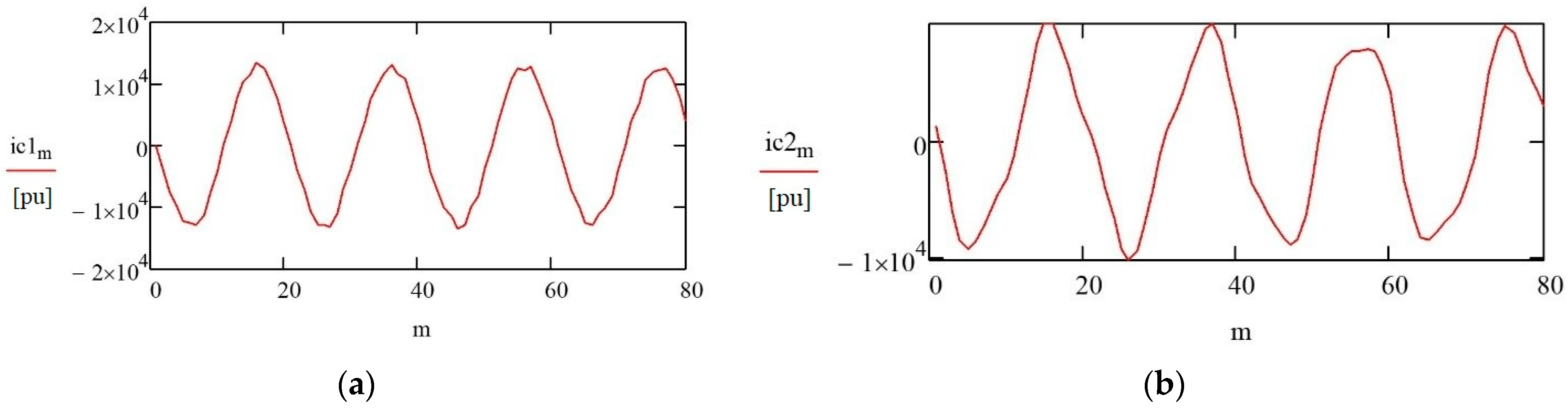
Let us assume that on the side of EPS1 (System-1) (Figure 1) the discrete instantaneous values of current i′(m) are distorted by flicker [63]. The distorted current signal i′(m) is illustrated in Figure 3a, and the mathematical expression for the instantaneous values of current taking into account the delay t_d corresponds to expression (22):

$$i^{\prime }\left(m\right)=I^{\prime }·(1-k·rnd(m\left)\right)·sin\left(2\pi ·f·\left(t_{delay}+m·t_d\right)\right),$$

(22)

where k—number (a constant coefficient) characterizing the “depth of distortion” of the flicker; rnd(m)—random number (for example, uniformly distributed in the interval [0; 1]), generated at each value of discrete time m.

Substituting numerical values into the example of the OHPL under consideration allows us to obtain expression (23):

$$i^{\prime }\left(m\right)=13908.15·(1-k·rnd(m\left)\right)·sin(2\pi ·50·(t_{delay}+m·t_d\left)\right),$$

(23)

and the realization of the current oscillogram at N = 20 (t_d = 10⁻³ s), k = 0.15 (15% of the amplitude I′), t_delay = 9 ∙ t_d = 9 ∙ 10⁻³ s is shown in Figure 3a.

The expression for instantaneous values of voltage u′(m) takes the form:

$$u^{\prime }\left(m\right)=U+I^{\prime }·(1-k·rnd(m\left)\right)·[n·R·sin(2\pi ·f·(t_{delay}+m·t_d))+n·L·cos(2\pi ·f·(t_{delay}+m·t_d)\left)\right] ,$$

(24)

Let us assume that there is a nonlinear load on the EPS2 (System-2) side (Figure 1) that emits, for example, an interharmonic into the electrical grid. To simplify the calculation, we assume that the instantaneous current values i″(m) are distorted by an interharmonic with a frequency of f_int = 135 Hz and an amplitude of I_int = 0.15 I″ at zero initial phase:

$$i^{″}\left(m\right)=I^{″}·sin(2\pi ·f·(t_{delay}+m·t_d\left)\right)+0.15·I^{″}·sin(2\pi ·f_{int}·(t_{delay}+m·t_d\left)\right),$$

(25)

The oscillogram of the current i″(m) for a given interharmonic distortion is shown in Figure 3b. The expression for calculating the instantaneous voltage values from the EPS2 side takes the following form:

$$\begin{gathered} u_{int}^{″}\left(m\right)=U+\left(1-n\right)·R·\left[I^{″}·\sin \left(2\pi ·f·\left(t_{delay}+m·t_d\right)\right)+0.15·I^{″}·\sin \left(2\pi ·f_{int}·\left(t_{delay}+m·t_d\right)\right)\right]+ \\ \hspace{1em}\hspace{1em}\hspace{1em}\hspace{1em}+ \left(1-n\right)·L·\left[I^{″}·\sin \left(2\pi ·f·\left(t_{delay}+m·t_d\right)\right)+0.15·I^{″}·\sin \left(2\pi ·f_{int}·\left(t_{delay}+m·t_d\right)\right)\right]. \end{gathered}$$

(26)

Thus, the calculation expression for determining the FL on OHPL in the presence of a flicker and interharmonic with a frequency of f_int = 135 Hz will correspond to expression (27):

$$\begin{gathered} n_{int}\left(m\right)=\left(u^{\prime }\left(m\right)-u_{int}^{″}\left(m\right)\right)+I^{″}·\left[R·\sin \left(2\pi ·f·\left(t_{delay}+m·t_d\right)\right)+L·\cos \left(2\pi ·f·\left(t_{delay}+m·t_d\right)\right)\right]+ \\ \hspace{1em}\hspace{1em}\hspace{1em}+ 0.15·I^{″}·[R·sin(2\pi ·f_{int}·(t_{delay}+m·t_d))+L·cos(2\pi ·f_{int}·(t_{delay}+m·t_d)\left)\right]/ \\ \left(I^{\prime }·\left(1-k·rnd\left(m\right)\right)+ I^{″}\right)·\left[R·\sin \left(2\pi ·f·\left(t_{delay}+m·t_d\right)\right)+L·\cos \left(2\pi ·f·\left(t_{delay}+m·t_d\right)\right)\right]+ \\ + 0.15·I^{″}·\left[R·\sin \left(2\pi ·f_{int}·\left(t_{delay}+m·t_d\right)\right)+L·\cos \left(2\pi ·f_{int}·\left(t_{delay}+m·t_d\right)\right)\right]. \end{gathered}$$

(27)

Substituting the numerical values in accordance with

Table 1. Values of calculated parameters.

Parameter	I′, A	I″, A	f, Hz	td, s	L, H	R, Ohm	fint, Hz	U, V	n
Value	13,908.15	9030.13	50	0.0025	0.0643	12.5	135	29,323.83	0.5

into expression (27) for k = 0.15 gives the following results:

• At m = 20; n_int(20) = 0.486; Δx = l ∙ (n − n_int) = 50 ∙ (0.5 − 0.486) = 0.7 km;
• At m = 60; n_int (60) = 0.526; Δx = l ∙ (n − n_int) = 50 ∙ (0.5 − 0.526) = −1.30 km.

Analysis of calculation results shows that errors in FL on OHPLs can have both positive and negative signs and be unevenly distributed across different points in time.

The accuracy of FL calculations on OHPLs, based on operating experience, is considered high if the error does not exceed the length of one span of the OHPL [64]. The span of a 110 kV OHPL is 0.15–0.2 km, so the required FL distance calculation accuracy is Δx = 0.2 km.

Consequently, in most calculation cases, given deviations in PQIs (flicker; interharmonics), most known methods for FL on OHPLs based on EMP, including those presented in [50], do not allow for the distance to the fault to be calculated with the required accuracy.

Therefore, it is necessary to develop a new method for detecting the FL on OHPLs using unsynchronized measurements from both ends of the line under conditions where the PQIs (currents and voltages) deviate from standard values.

3. Results

Let us consider the feasibility and effectiveness of applying the least-squares method (LSM) to the problem of FL on OHPLs under conditions where PQIs deviate from standard values.

3.1. Algorithm of Actions

To implement the method for FL on OHPLs, applicable both to currents and voltages that deviate from a sinusoidal shape and to those that do not, we propose performing the following set of steps:

• Take measurements from both ends of the OHPL of the instantaneous values of phase currents (i′_A, i′_B, i′_C), (i″_A, i″_B, i″_C) and voltages (u′_A, u′_B, u′_C), (u″_A, u″_B, u″_C) at the moment of a SC, not synchronized in time;
• Determine the faulted phase(s) and obtain oscillograms of currents and voltages;
• Ensure synchronization of instantaneous values of currents and voltages by combining oscillograms of the emergency mode from both ends of the OHPL at the onset of the SC;
• Select, over an interval of two to ten periods from the onset of the SC, and form arrays of M (m = 1, …, M) consecutive instantaneous values for each of the oscillograms of the current and voltage of the faulted phase i′(m), i″(m), u′(m), u″(m);
• Determine the first derivatives of currents with respect to time for the selected arrays of instantaneous values di′(m)/dt_m, di″(m)/dt_m, as well as the first and second derivatives of voltages du′(m)/dt_m, du″(m)/dt_m, d²u′(m)/dt²_m, d²u″(m)/dt²_m;
• Form the voltage matrices U1 and U2 using the active resistance R, inductance L and transverse capacitance C of the OHPL, instantaneous values of the current and voltage arrays i′(m), i″(m), u′(m), u″(m), as well as the calculated instantaneous values of the derivatives of the currents and voltages di′(m)/dt_m, di″(m)/dt_m, du′(m)/dt_m, du″(m)/dt_m, d²u′(m)/dt²_m, d²u″(m)/dt²_m according to the expressions:

$$\mathbf{U}\mathsf{1}=‖\begin{array}{c}\mathrm{U}1\left(1\right)\\ \mathrm{U}1\left(2\right)\\ ··· \\ \mathrm{U}1\left(M\right)\end{array}‖,$$

$$\mathbf{U}\mathsf{2}=‖\begin{array}{c}\mathrm{U}2\left(1\right)\\ \mathrm{U}2\left(2\right)\\ ··· \\ \mathrm{U}2\left(M\right)\end{array}‖,$$

where:

$$\mathrm{U}1\left(m\right)=R·\left(i^{\prime }\left(m\right)+i^{″}\left(m\right)\right)+L·\left({\displaystyle \frac{{di}^{\prime }\left(m\right)}{{dt}_m}}+{\displaystyle \frac{{di}^{″}\left(m\right)}{{dt}_m}}\right)-R·C·\left({\displaystyle \frac{d{u}^{\prime }\left(m\right)}{{dt}_m}}+{\displaystyle \frac{d{u}^{″}\left(m\right)}{{dt}_m}}\right)-L·C·({\displaystyle \frac{d^2{u}^{\prime }\left(m\right)}{{dt}_m^2}} + {\displaystyle \frac{d^2{u}^{″}\left(m\right)}{{dt}_m^2}});$$

$$\mathrm{U}2\left(m\right)=\left[u^{\prime }\left(m\right)-u^{″}\left(m\right)\right]+i^{″}\left(m\right)·R+L·{\displaystyle \frac{{di}^{″}\left(m\right)}{{dt}_m}}-R·C·{\displaystyle \frac{d{u}^{″}\left(m\right)}{{dt}_m}}-L·C·{\displaystyle \frac{d^2{u}^{″}\left(m\right)}{{dt}_m^2}}.$$

• Determine the relative value of the distance to the SC location n using the voltage matrices U1 and U2 and the least-squares method according to the expression:

$$n={\left({\mathbf{U}\mathsf{1}}^{\mathrm{T}}\mathbf{U}\mathsf{1}\right)}^{-1}·{\mathbf{U}\mathsf{1}}^{\mathrm{T}}·\mathbf{U}\mathsf{2};$$

• Based on the obtained relative value of the distance to the SC location n, determine the distance to the FL from the end of the OHPL with index “ ′ ”.

Let us explain the above steps for processing current and voltage signals, which are necessary for the implementation of the developed new method for determining the FL on OHPLs using unsynchronized measurements from both ends.

Let us introduce a discrete time variable and group the components of the expression, writing it as follows:

$$\begin{gathered} \left[u^{\prime }\left(m\right)-u^{″}\left(m\right)\right]+i^{″}\left(m\right)·R+L·{\displaystyle \frac{{di}^{″}\left(m\right)}{{dt}_m}}-R·C·{\displaystyle \frac{d{u}^{″}\left(m\right)}{{dt}_m}}-L·C·{\displaystyle \frac{d^2{u}^{″}\left(m\right)}{{dt}_m^2}}= \\ \hspace{1em}\hspace{1em}\hspace{1em}= n·[R·(i^{\prime }\left(m\right)+i^{″}\left(m\right))+L·({\displaystyle \frac{{di}^{\prime }\left(m\right)}{{dt}_m}}+{\displaystyle \frac{{di}^{″}\left(m\right)}{{dt}_m}})-R·C ·({\displaystyle \frac{d{u}^{\prime }\left(m\right)}{{dt}_m}} + {\displaystyle \frac{d{u}^{″}\left(m\right)}{{dt}_m}})- \\ - L·C·({\displaystyle \frac{d^2{u}^{\prime }\left(m\right)}{{dt}_m^2}} + {\displaystyle \frac{d^2{u}^{″}\left(m\right)}{{dt}_m^2}})]. \end{gathered}$$

(28)

where m—discrete variable corresponding to the moments of time of the current and voltage oscillogram readings; m = 1, 2, …, M, where M—number of readings that make up the current (voltage) selected for the implementation of digital signal processing operations of the method for determining the FL on OHPL.

Let us denote by column matrices U1 and U2 the expressions for different moments of discrete time m, included in expression (28):

$$\mathbf{U}\mathsf{1}=‖\begin{array}{c}\mathrm{U}1\left(1\right)\\ \mathrm{U}1\left(2\right)\\ ··· \\ \mathrm{U}1\left(M\right)\end{array}‖,$$

(29)

$$\mathbf{U}\mathsf{2}=‖\begin{array}{c}\mathrm{U}2\left(1\right)\\ \mathrm{U}2\left(2\right)\\ ··· \\ \mathrm{U}2\left(M\right)\end{array}‖.$$

(30)

Thus, for the realizations of expression (28) at different moments of time m, the following matrix expression (31) is valid:

$$\mathbf{U}\mathsf{1}·n=\mathbf{U}\mathsf{2}.$$

(31)

To find a more accurate value of n that represents the SC location on an OHPL under conditions where currents and voltages deviate from a sinusoidal shape, we use the LSM. This method uses a full set of M discrete realizations of currents and voltages (expression (31)). It minimizes the error in FL determination caused by random factors. This differs from the method in [50], which only uses individual “time slices” of oscillograms.

Let us write expression (31) as:

$$\mathbf{U}\mathsf{1}·n=\mathbf{U}\mathsf{2}+\mathbf{e},$$

(32)

where e—column vector of measurement errors associated with distorted instantaneous values of the current and voltage waveforms.

The problem of minimizing errors when calculating n is reduced to minimizing the squared norm of the error vector e, that is:

$${\sum }_{m=1}^M{e}_m·e_m={\parallel e\parallel }^2={\mathbf{e}}^{\mathrm{T}}·\mathbf{e}.$$

(33)

Let us transform expression (33) using substitution (32):

$$\mathbf{U}\mathsf{1}·n -\mathbf{U}\mathsf{2}=\mathbf{e},$$

(34)

then:

$${\mathbf{e}}^T·\mathbf{e}={(\mathbf{U}\mathsf{1}·n-\mathbf{U}\mathsf{2})}^{\mathrm{T}}·(\mathbf{U}\mathsf{1}·n-\mathbf{U}\mathsf{2})={\mathbf{U}\mathsf{1}}^{\mathrm{T}}·n·\mathbf{U}\mathsf{1}·n-2{\mathbf{U}\mathsf{1}}^{\mathrm{T}}·n·\mathbf{U}\mathsf{2}+{\mathbf{U}\mathsf{2}}^{\mathrm{T}}·\mathbf{U}\mathsf{2}.$$

(35)

To find the minimum, it is necessary to calculate the partial derivative with respect to n of Equation (35) and equate it to zero:

$$\partial {\mathbf{e}}^T·\mathbf{e}/\partial n=2·{\mathbf{U}\mathsf{1}}^{\mathrm{T}}·\mathbf{U}\mathsf{1}·n-2 {\mathbf{U}\mathsf{1}}^{\mathrm{T}}·\mathbf{U}\mathsf{2} = 0.$$

(36)

From the last relation we find the desired value of n in accordance with expression (37):

$$n={({\mathbf{U}\mathsf{1}}^{\mathrm{T}}·\mathbf{U}\mathsf{1})}^{-1}·{\mathbf{U}\mathsf{1}}^{\mathrm{T}}·\mathbf{U}\mathsf{2}.$$

(37)

Thus, estimating the relative distance to a SC on an OHPL under conditions of current and voltage deviations from a sinusoidal shape using the LSM is reduced to finding the results of the matrix product using expression (37).

3.2. Second Calculated Example

Let us illustrate with an example the calculation of the distance to the SC under the above-discussed conditions of current distortion i′(m) by a flicker (Figure 3a), as well as i″(m) by an interharmonic with a frequency of f_int = 135 Hz and an amplitude of I_int = 0.15 I″ (Figure 3b). According to previously obtained expressions (22)–(27), for the introduced delay t_delay, matrices U1 and U2 take the form:

$$\mathbf{U}\mathsf{1}=‖\begin{array}{c}\mathrm{U}1\left(1\right)\\ \mathrm{U}1\left(2\right)\\ ··· \\ \mathrm{U}1\left(M\right)\end{array}‖,$$

(38)

$$\mathbf{U}\mathsf{2}=‖\begin{array}{c}\mathrm{U}2\left(1\right)\\ \mathrm{U}2\left(2\right)\\ ··· \\ \mathrm{U}2\left(M\right)\end{array}‖,$$

(39)

where:

$$\begin{gathered} \mathrm{U}1\left(m\right)=\left(I^{\prime }·\left(1-k·rnd\left(m\right)\right)+ I^{″}\right)·\left[R·sin\left(2\pi ·f·\left(t_{delay}+m·t_d\right)\right)+L·cos\left(2\pi ·f·\left(t_{delay}+m·t_d\right)\right)\right]+ \\ \hspace{1em}\hspace{1em}\hspace{1em} + 0.15·I^{″}·\left[R·sin\left(2\pi ·f_{int}·\left(t_{delay}+m·t_d\right)\right)+L·cos\left(2\pi ·f_{int}·\left(t_{delay}+m·t_d\right)\right)\right]- \\ \hspace{1em}\hspace{1em}\hspace{1em}\hspace{1em}\hspace{1em}\hspace{1em}\hspace{1em}\hspace{1em}\hspace{1em}\hspace{1em}- R·C ·\left({\displaystyle \frac{d{u}^{\prime }\left(m\right)}{{dt}_m}} + {\displaystyle \frac{{du}_{int}^{″}\left(m\right)}{{dt}_m}}\right)-L·C·({\displaystyle \frac{d^2{u}^{\prime }\left(m\right)}{{dt}_m^2}} + {\displaystyle \frac{d^2{u}_{int}^{″}\left(m\right)}{{dt}_m^2}}); \end{gathered}$$

$$\begin{gathered} \mathrm{U}2\left(m\right)=\left[\right(u^{\prime }\left(m\right)-u_{int}^{″}\left(m\right))+I^{″}·[R·sin(2\pi ·f·(t_{delay}+m·t_d\left)\right)+L·cos(2\pi ·f·(t_{delay}+m·t_d\left)\right)]+ \\ +0.15·I^{″}·[R·\mathrm{s}\mathrm{i}\mathrm{n}(2\pi ·f_{int}·(t_{delay}+m·t_d))+L·\mathrm{c}\mathrm{o}\mathrm{s}(2\pi ·f_{int}·(t_{delay}+m·t_d)\left)\right]]- \\ \hspace{1em}\hspace{1em}-R·C· {\displaystyle \frac{{du}_{int}^{″}\left(m\right)}{{dt}_m}}-L·C·{\displaystyle \frac{d^2{u}_{int}^{″}\left(m\right)}{{dt}_m^2}}; \end{gathered}$$

$$u^{\prime }\left(m\right)=U+I^{\prime }·(1-k·rnd(m\left)\right)·[n·R·sin(2\pi ·f·(t_{delay}+m·t_d))+n·L·cos(2\pi ·f·(t_{delay}+m·t_d)\left)\right];$$

$$\begin{gathered} u_{int}^{″}\left(m\right)=U+(1-n)·R·[I^{″}·sin(2\pi ·f·(t_{delay}+m·t_d))+0.15·I^{″}·sin(2\pi ·f_{int}·(t_{delay}+m·t_d)\left)\right]+ \\ +(1-n)·L·[I^{″}·sin(2\pi ·f·(t_{delay}+m·t_d))+0.15·I^{″}·sin(2\pi ·f_{int}·(t_{delay}+m·t_d)\left)\right]; \end{gathered}$$

$${\displaystyle \frac{d{u}^{\prime }\left(m\right)}{{dt}_m}}={\displaystyle \frac{(u^{\prime }\left(m+1\right)-u^{\prime }(m-1\left)\right)}{2·t_d}};\hspace{1em}{\displaystyle \frac{{du}_{int}^{″}\left(m\right)}{{dt}_m}}={\displaystyle \frac{(u_{int}^{″}\left(m+1\right)-{ u}_{int}^{″}(m-1\left)\right)}{2·t_d}};$$

$${\displaystyle \frac{d^2{u}^{\prime }\left(m\right)}{{dt}_m^2}}={\displaystyle \frac{\left(u^{\prime }\right(m+1)-2·u^{\prime }\left(m\right)+u^{\prime }(m-1\left)\right)}{t_d^2}};$$

$${\displaystyle \frac{d^2{u}_{int}^{″}\left(m\right)}{{dt}_m^2}}={\displaystyle \frac{(u_{int}^{″}\left(m+1\right)-2·u_{int}^{″}\left(m\right)+u_{int}^{″}(m-1\left)\right)}{t_d^2}}.$$

The numerical values of the parameters for the calculations are presented in Table 1. The specific transverse (capacitive) conductivity C_linear of the 110 kV OHPL (Figure 2) was selected according to [65]. The capacitance of the OHPL C for the calculations was:

$$b=2\pi ·f·C_{linear}=1.25·{10}^{-6} \mathrm{cm}/\mathrm{km}; C=C_{linear}·l={\displaystyle \frac{b·l}{2\pi ·f}}=198.9·{10}^{-9} \mathrm{F}.$$

(40)

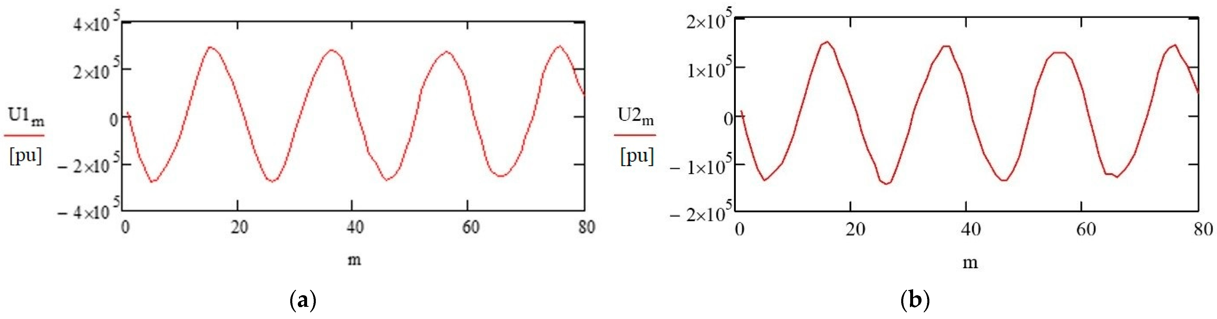
Discrete values of matrices U1 and U2 (expressions (38) and (39)) correspond to instantaneous values of voltage oscillograms shown in Figure 4. To implement FL on OHPLs, it is necessary to set the value of variable M, which determines the number of discrete current and voltage samples used in least-squares calculations. It is advisable to select the value of M as a multiple of N, the number of samples per industrial frequency period (e.g., N = 20), and the total sample size of successive instantaneous current and voltage values, as in [50], is within the interval of two to ten periods from the onset of the SC for the current and voltage oscillograms of the faulted phase. We select the value of M = 80, and the delay relative to the onset of the SC is taken to be t_delay = 9 ∙ t_d = 0.0225 s, k = 0.15.

Calculations of the distance to the SC location on OHPL under conditions of current and voltage deviations from a sinusoidal shape with the substitution of the values of M, t_delay, as well as the parameter values into expressions (38) and (39) in the MATCAD software package (version 15). The final calculation results, corresponding to the oscillograms in Figure 3 and Figure 4 and expression (37), made it possible to obtain a more accurate relative distance to the SC location on OHPL:

$${ n}_{int}={\left({\mathbf{U}\mathsf{1}}^{\mathrm{T}}\mathbf{U}\mathsf{1}\right)}^{-1}·{\mathbf{U}\mathsf{1}}^{\mathrm{T}}·\mathbf{U}\mathsf{2}=0.499.$$

Taking into account previously performed calculations, the error in determining the FL on OHPL was:

$$\Delta x=l·(n-{ n}_{int})=50·(0.5-0.499)=-0.05 \mathrm{km},$$

or (for a transmission line length of l = 50 km) the value −0.05/50 = −0.1% of the length of the OHPL, which indicates the high accuracy of the newly developed method for determining the FL on OHPLs.

4. Discussion

In modern power systems, deviations in PQIs from standard values are possible due to the widespread adoption of various types of power electronics. When PQI deviations occur, FL devices on OHPLs can produce significant measurement errors, leading to increased time spent locating and repairing the fault [66,67,68]. Extended outages of OHPLs lead to a decrease in the reliability of the overall power system [69,70,71].

A new method for FL on OHPLs has been developed. It uses unsynchronized measurements from both ends and accounts for deviations in current and voltage from a sinusoidal shape. The method is based on the LSM and provides highly accurate distance calculations to the fault. Comparative calculation results presented in the article confirm that even when PQIs deviate from standard values, the accuracy of the distance calculation meets operational requirements. For 110 kV OHPLs, the error must not exceed the length of one span, which is 0.15–0.2 km. In the example considered, the error does not exceed 0.05 km. This new FL method can be implemented in practice. It works with most modern digital protection and automation terminals produced by various manufacturers. These terminals are interconnected by a communication channel for exchanging current and voltage oscillograms [72,73]. Requirements for such terminals are provided in [74], which mandate the implementation of an FL function for OHPLs. No hardware modifications to the terminals are required. Only software modifications are needed.

It is possible to implement the developed new method for FL on OHPLs in the software of power system control centers. This is due to the fact that the calculation of the distance to the FL is entrusted to the control personnel who are in charge of the OHPLs. At the same time, remote collection of fault tracings (currents and voltages) is carried out from emergency event recorders (digital protection and automation terminals) on both sides of the OHPL to calculate the distance to the FL [75,76,77,78].

5. Conclusions

Given the deviations of PQIs (currents and voltages from sinusoidal waveforms) from standard values in modern power systems, the development of new fault location methods for OHPLs that ensure high-accuracy distance calculations is a pressing issue.

A new fault location method for OHPLs has been developed using unsynchronized measurements from both ends. This method allows for the accuracy of distance calculations to OHPLs FL of 0.1% (0.05 km) of the line’s length, which meets operational requirements. Using existing fault location methods for OHPLs, which do not take into account deviations of PQIs from standard values, the accuracy of distance calculations to the FL, using the same initial data, is 1.4–2.6% (0.7–1.3 km, respectively), which is 3.5–8.7 times greater than the span length of an OHPL (0.15–0.2 km).

FL errors for OHPLs can be significantly reduced—by a factor of 14 to 26—when PQIs deviate from standard values. This reduction is achieved in two ways. First, additional OHPL parameters are used. Second, the LSM is applied to calculations based on instantaneous current and voltage values from emergency oscillograms. Transverse (capacitive) admittance is used as an additional parameter. It ensures high accuracy in FL detection for OHPLs. In addition, the new FL method uses differential equations. These equations describe fault currents and voltages recorded at both ends of the OHPL.

The new fault location method for OHPLs can be implemented in existing digital protection and automation terminals from various manufacturers, as well as in the software of power system control centers.

References

1. Voropai, N. Electric Power System Transformations: A Review of Main Prospects and Challenges. Energies 2020, 13, 5639. [Google Scholar] [CrossRef]
2. Suliman, A.S.; Ahmed, B.M.; Elareefi, M.B.; Elrahman, E.A.E.A.; Arbab, E.A.; Abdulwahab, M.M. Monitoring System for Overhead Power Transmission Lines in Smart Grid System Using Internet of Things. Univ. Khartoum Eng. J. 2022, 12, 1. [Google Scholar] [CrossRef]
3. Farkhadzeh, E.M.; Muradaliev, A.Z.; Abdullaeva, S.A.; Nazarov, A.A. Quantitative Assessment of the Operational Reliability of Overhead Power Transmission Lines. Power Technol. Eng. 2022, 55, 790–796. [Google Scholar] [CrossRef]
4. Nazemi, M.; Dehghanian, P.; Darestani, Y.; Su, J. Parameterized Wildfire Fragility Functions for Overhead Power Line Conductors. Power Syst. IEEE Trans. Power Syst. 2023, 99, 2517–2527. [Google Scholar] [CrossRef]
5. Gonçalves, A.C.R.; Marques, M.C.; Loureiro, S.; Nieto, R.; Liberato, M.L.R. Disruption risk analysis of the overhead power lines in Portugal. Energy 2022, 263, 125583. [Google Scholar] [CrossRef]
6. Listyukhin, V.; Pecherskaya, E.; Gurin, S.; Anisimova, A.; Shepeleva, A. Analysis and classification of cause and effect factors affecting the operating modes of overhead power lines. AIP Conf. Proc. 2022, 2767, 020019. [Google Scholar] [CrossRef]
7. Savina, N.V.; Varygina, A.O. Selection of an optimal cable brand for high-voltage overhead power lines based on criterion analysis. Ipolytech J. 2023, 27, 339–353. [Google Scholar] [CrossRef]
8. Korotkevich, M.A.; Podgaisky, S.I. On the Expediency of Laying Cable Power Lines with a Voltage of 6–35 kV Outside Settlements Instead of Overhead Power Lines. Energetika 2022, 65, 463–476. [Google Scholar] [CrossRef]
9. Listyukhin, V.A.; Pecherskaya, E.A.; Artamonov, D.; Zinchenko, T.O.; Anisimova, A.A. Improving the reliability of overhead power transmission lines through the introduction of information and measurement systems for monitoring their parameters. Meas. Monit. Manag. Control 2022, 3, 62–68. (In Russian) [Google Scholar] [CrossRef]
10. Li, P.; Qiu, R.; Wang, M.; Wang, X.; Jaffry, S.; Xu, M.; Huang, K.; Huang, Y. Online Monitoring of Overhead Power Lines Against Tree Intrusion via a Low-cost Camera and Mobile Edge Computing Approach. J. Phys. Conf. Ser. 2023, 2422, 012018. [Google Scholar] [CrossRef]
11. Ilyushin, P.; Volnyi, V.; Suslov, K.; Filippov, S. Review of Methods for Addressing Challenging Issues in the Operation of Protection Devices in Microgrids with Voltages of up to 1 kV that Integrates Distributed Energy Resources. Energies 2022, 15, 9186. [Google Scholar] [CrossRef]
12. Powanga, L.; Kwakwa, P.A. Determinants of Electricity Transmission and Distribution Losses in South Africa. J. Renew. Energy 2023, 2023, 2376449. [Google Scholar] [CrossRef]
13. Thomas, D.; Fung, J. Measuring downstream supply chain losses due to power disturbances. Energy Econ. 2022, 114, 106314. [Google Scholar] [CrossRef]
14. Gurevich, Y.E.; Kabikov, K.V. Peculiarities of Power Supply, Aimed at Failure-Free Operation of Industrial Consumers; ELEKS-KM: Moscow, Russia, 2005. (In Russian) [Google Scholar]
15. Bollen, M.H.J.; Dirix, P.M.E. Simple model for post-fault motor behaviours for reliability/power quality assessment of industrial power systems. IEE Proc.–Gener. Transm. Distrib. 1996, 143, 56–60. [Google Scholar] [CrossRef]
16. Eroshenko, S.A.; Ilyushin, P.V. Features of implementing multi-parameter islanding protection in power districts with distributed generation units. In Proceedings of the 2018 IEEE 59th International Scientific Conference on Power and Electrical Engineering of Riga Technical University (RTUCON), Riga, Latvia, 12–14 November 2018. [Google Scholar] [CrossRef]
17. Won, D.J.; Chung, I.Y.; Kim, J.M.; Moon, S.I.; Seo, J.C.; Choe, J.W. A new algorithm to locate power-quality event source with improved realization of distributed monitoring scheme. IEEE Trans. Power Deliv. 2006, 21, 1641–1647. [Google Scholar] [CrossRef]
18. Kulikov, A.L.; Shepovalova, O.V.; Ilyushin, P.V.; Filippov, S.P.; Chirkov, S.V. Control of Electric Power Quality Indicators in Distribution Networks Comprising a High Share of Solar Photovoltaic and Wind Power Stations. Energy Rep. 2022, 8, 1501–1514. [Google Scholar] [CrossRef]
19. Kulikov, A.L.; Ilyushin, P.V.; Suslov, K.V.; Karamov, D.N. Coherence of Digital Processing of Current and Voltage Signals at Decimation for Power Systems with a Large Share of Renewable Power Stations. Energy Rep. 2022, 8, 1464–1478. [Google Scholar] [CrossRef]
20. Koks, E.E.; Pant, R.; Thacker, S.; Hall, J. Understanding Business Disruption and Economic Losses Due to Electricity Failures and Flooding. Int. J. Disaster Risk Sci. 2019, 10, 421–438. [Google Scholar] [CrossRef]
21. Lacommare, K.; Eto, J. Cost of power interruptions to electricity consumers in the United States (US). Energy 2006, 31, 1845–1855. [Google Scholar] [CrossRef]
22. Edomah, N. Effects of voltage sags, swell and other disturbances on electrical equipment and their economic implications. In Proceedings of the 20th International Conference and Exhibition on Electricity Distribution, Prague, Czech Republic, 8–11 June 2009; pp. 1–4. [Google Scholar]
23. Saha, M.M.; Izykowski, J.; Rosolowski, E. Fault Location on Power Networks; Springer: London, UK, 2010; 437p. [Google Scholar]
24. Kezunovic, M.; Knezev, M. Selection of optimal fault location algorithm. In 2008 IEEE Power and Energy Society General Meeting—Conversion and Delivery of Electrical Energy in the 21st Century; IEEE: New York, NY, USA, 2008. [Google Scholar] [CrossRef]
25. Maly, A.S.; Shalyt, G.M.; Eisenfeld, A.I. Determination of the Places of Damage to Power Transmission Lines According to the Parameters of the Emergency Mode; Energiya: Moscow, Russia, 1972; 215p. (In Russian) [Google Scholar]
26. Panahi, H.; Zamani, R.; Sanaye-Pasand, M.; Mehrjerdi, H. Advances in Transmission Network Fault Location in Modern Power Systems: Review, Outlook and Future Works. IEEE Access 2021, 9, 158599–158615. [Google Scholar] [CrossRef]
27. Arbuzov, R.S.; Ovsyannikov, A.G. Modern Diagnostic Methods of Overhead Power Transmission Lines; Nauka Publ.: Novosibirsk, Russia, 2009; 136p. (In Russian) [Google Scholar]
28. Shalyt, G.M. Determination of the Place of Damage in Electrical Networks; Energoatomizdat: Moscow, Russia, 1982; 312p. (In Russian) [Google Scholar]
29. Krzysztof, G.; Kowalik, R.; Rasolomampionona, D.D.; Anwar, S. Traveling wave fault location in power transmission systems: An overview. J. Electr. Syst. 2011, 7, 287–296. [Google Scholar]
30. Lachugin, V.F. Wave methods for determining the location of damage on overhead power lines. Relay Prot. Autom. 2023, 1, 58–61. (In Russian) [Google Scholar]
31. Lachugin, V.F.; Platonov, P.S.; Alekseev, V.G.; Vazyulin, M.V.; Mitrofanov, N.N.; Popov, S.G.; Izmukov, G.N.; Podshivalin, A.N.; Artyunov, S.A.; Klyushkin, N.G.; et al. Field Tests of a Traveling Wave Fault Location Service for Overhead Transmission Lines. Power Technol. Eng. 2022, 55, 783–789. [Google Scholar] [CrossRef]
32. Hsu, W.T.; Huang, Q.; Huang, C.W.; Yang, C.C. Fault Location Detection Using CEEMD and Two-Terminal Traveling Wave Ranging. Fluct. Noise Lett. 2026. [Google Scholar] [CrossRef]
33. Minullin, R.G. Detecting the faults of overhead electric-power lines by the location-probing method. Russ. Electr. Eng. 2017, 88, 61–70. [Google Scholar] [CrossRef]
34. Arzhannikov, E.A.; Lukoyanov, V.Y.; Misrikhanov, M.S. Determining the Location of a Short Circuit on High−Voltage Power Transmission Lines; Shuin, V.A., Ed.; Energoatomizdat: Moscow, Russia, 2003; 272p. (In Russian) [Google Scholar]
35. Kulikov, A.; Ilyushin, P.; Loskutov, A.; Filippov, S. Application of Search Algorithms in Determining Fault Location on Overhead Power Lines According to the Emergency Mode Parameters. Algorithms 2023, 16, 189. [Google Scholar] [CrossRef]
36. Visyashchev, A.N. Devices and Methods for Determining the Location of Damage on Power Transmission Lines: A Textbook; At 2 h. h. 1; Publishing House of IrSTU: Irkutsk, Russia, 2001; 188p. (In Russian) [Google Scholar]
37. Lebedev, V.; Filatova, G.; Timofeev, A. Increase of accuracy of the fault location methods for overhead electrical power lines. Adv. Mater. Sci. Eng. 2018, 2018, 3098107. [Google Scholar] [CrossRef]
38. Kulikov, A.; Ilyushin, P.; Loskutov, A.; Filippov, S. Fault Location Method for Overhead Power Line Based on a Multi-Hypothetical Sequential Analysis Using the Armitage Algorithm. Inventions 2023, 8, 123. [Google Scholar] [CrossRef]
39. Kosyakov, A.A.; Kuleshov, P.V.; Pogudin, A.L. The influence of the grounding device structure of a substation on the voltage of conducted interference of lightning currents. Russ. Electr. Eng. 2019, 90, 752–755. [Google Scholar] [CrossRef]
40. Sharipov, U.B.; Égamnazarov, G.A. Calculating currents in lightning protection cables and in optical cables built into them during asymmetric short circuits in overhead transmission lines. Power Technol. Eng. 2017, 50, 673–678. [Google Scholar] [CrossRef]
41. Shevchenko, N.Y.; Ugarov, G.G.; Kirillova, S.N.; Lebedeva, Y.V. Review and analysis of the design features of overhead power line wires with increased resistance to icy-wind loads. Quest. Electr. Technol. 2018, 4, 53–63. (In Russian) [Google Scholar]
42. Ahmedova, O.; Soshinov, A.; Shevchenko, N. Analysis of influence of external atmospheric factors on the accuracy of fault location on overhead power lines. E3S Web Conf. 2020, 178, 01057. [Google Scholar] [CrossRef]
43. Wang, D.; Yu, D.; Gao, H.; Peng, F.; Lin, J.; Wang, J.; Hou, M. Frequency Modification Algorithm-Based Traveling Wave Fault Location Approach for Overhead Transmission Lines with Structural Changes. Prot. Control Mod. Power Syst. 2025, 10, 1–12. [Google Scholar] [CrossRef]
44. Ustinov, A.A.; Visyashchev, A.N. Iterative methods for determining the location of damage by emergency mode parameters during one-way measurements on overhead power transmission lines. Bull. IrSTU 2010, 5, 260–266. (In Russian) [Google Scholar]
45. Minullin, R.G.; Granskaya, A.A.; Abdullazyanov, E.Y.; Akhmetova, I.G.; Mustafin, R.G.; Kasimov, V.A. Connecting methods of location monitoring equipment to overhead power lines. Power Eng. Res. Equip. Technol. 2024, 26, 16–32. (In Russian) [Google Scholar] [CrossRef]
46. Xu, P.; Zhou, R. Research on Fault Location Methods for Multi-Terminal Multi-Section Overhead Line–Cable Hybrid Transmission Lines. Processes 2026, 14, 438. [Google Scholar] [CrossRef]
47. Zhang, X.; Xu, B.; Han, Z.; Shi, F. Improvement of Traveling Wave-Based Fault Location Method for Overhead Distribution Lines. Prot. Control Mod. Power Syst. 2026, 11, 157–172. [Google Scholar] [CrossRef]
48. Ilyushin, P.V.; Sukhanov, O.A. The structure of emergency-management systems of distribution networks in large cities. Russ. Electr. Eng. 2014, 85, 133–137. [Google Scholar] [CrossRef]
49. STO 56947007-29.240.55.224-2016; Guidelines for Determining Damage to Overhead Lines with a Voltage of 110 kV and Above. PJSC FGC UES: Moscow, Russia, 2016. (In Russian)
50. Visyashchev, A.N.; Plenkov, E.R.; Tiguntsev, S.G. Method for Determining the Location of a Short Circuit on an Overhead Power Transmission Line with Unsynchronized Measurements from Two of Its Ends. RU 2508556, 27 February 2014. [Google Scholar]
51. Mokeev, A.V.; Piskunov, S.A. Application of synchronized vector measurement technology to improve remote protection. Relay Prot. Autom. 2022, 3, 12–17. (In Russian) [Google Scholar]
52. Ayambire, P.N. Magnetic Sensor-Based Approach for Overhead Transmission Lines Fault Detection and Location Using Line Fault Current. Turk. J. Electr. Power Energy Syst. 2025, 5, 132–141. [Google Scholar] [CrossRef]
53. Ilyushin, P.V.; Pazderin, A.V. Approaches to Organization of Emergency Control at Isolated Operation of Energy Areas with Distributed Generation. In Proceedings of the 2018 International Ural Conference on Green Energy (UralCon), Chelyabinsk, Russia, 4–6 October 2018; pp. 149–155. [Google Scholar] [CrossRef]
54. Bahmanyar, A.; Jamali, S.; Estebsari, A.; Bompard, E. A comparison framework for distribution system outage and fault location methods. Electr. Power Syst. Res. 2017, 145, 19–34. [Google Scholar] [CrossRef]
55. Schweitzer, E.O. A review of impedance-based fault locating experience. In Proceedings of the 14th Annual Iowa–Nebraska System Protection Seminar; Iowa–Nebraska System Protection Seminar: Omaha, NE, USA, 1990; pp. 1–31. [Google Scholar]
56. Stringfield, T.W.; Marihart, D.J.; Stevens, R.F. Fault location methods for overhead lines. IEEE Trans. Power Appar. Syst. 1957, 76, 518–530. [Google Scholar] [CrossRef]
57. Senderovich, G.A.; Gryb, O.G.; Karpaliuk, I.T.; Shvets, S.V.; Zaporozhets, A.O.; Samoilenko, I.A. Experimental studies of the method for determining location of damage of overhead power lines in the operation mode. Stud. Syst. Decis. Control 2021, 359, 55–77. [Google Scholar]
58. Gurevich, Y.E.; Libova, L.E. Application of Mathematical Models of Electrical Load in Calculation of the Power Systems Stability and Reliability of Power Supply to Industrial Enterprises; ELEKS-KM: Moscow, Russia, 2008. (In Russian) [Google Scholar]
59. Ilyushin, P.; Filippov, S.; Kulikov, A.; Suslov, K.; Karamov, D. Intelligent Control of the Energy Storage System for Reliable Operation of Gas-Fired Reciprocating Engine Plants in Systems of Power Supply to Industrial Facilities. Energies 2022, 15, 6333. [Google Scholar] [CrossRef]
60. Yu, C.S.; Liu, C.W.; Jiang, J.A. A new fault location algorithm for series compensated lines using synchronized phasor measurements. In Proceedings of the 2000 Power Engineering Society Summer Meeting, Washington, DC, USA, 16–20 July 2000. [Google Scholar] [CrossRef]
61. Kezunovic, M.; Meliopoulos, S.; Venkatasubramanian, V.; Vittal, V. Application of Time-Synchronized Measurements in Power System Transmission Networks; Springer: New York, NY, USA, 2014. [Google Scholar]
62. Aboshady, F.M.; Thomas, D.W.P. A Wideband Single End Fault Location Scheme for Active Untransposed Distribution Systems. IEEE Trans. Smart Grid 2020, 11, 2115–2124. [Google Scholar] [CrossRef]
63. GOST 32144-2013; Electrical Energy. Electromagnetic Compatibility of Technical Means. Electrical Energy Quality Standards in General–Purpose Power Supply Systems. Standartinform: Moscow, Russia, 2013. (In Russian)
64. STO 56947007-29.240.55.159-2013; Standard Instructions for the Organization of Work to Identify Damage to Overhead Power Lines with a Voltage of 110 kV and Above. PJSC FGC UES: Moscow, Russia, 2013. (In Russian)
65. Panova, E.A.; Albrecht, A.Y. Refined specific electrical parameters of double-circuit 110 kV power lines for remote damage location detection. Electr. Eng. Syst. Complexes 2016, 4, 35–40. (In Russian) [Google Scholar]
66. Takagi, T.; Yamakoshi, Y.; Yamaura, Y.; Kondow, R.; Matsushima, T. Development of a new type fault locator using the one-terminal voltage and current data. IEEE Trans. Power Appar. Syst. 1982, PAS-101, 2892–2898. [Google Scholar] [CrossRef]
67. Simeon, O.; Faithpraise, F.O.; Ibanga, J. Iterative Newton-Raphson-Based Impedance Method for Fault Distance Detection on Transmission Line. Int. Multiling. J. Sci. Technol. 2020, 5, 2805–2810. [Google Scholar] [CrossRef]
68. Nagendra Reddy, P.L.V.; Mukunda, V.K.S.; Sushyanth, C.; Vanitha, V. Implementation of Novosel Simple Impedance Algorithm for fault location. IJCTA 2016, 9, 7589–7596. [Google Scholar]
69. Liao, Y. Transmission Line Fault Location Algorithms Without Requiring Line Parameters. Electr. Power Compon. Syst. 2008, 36, 1218–1225. [Google Scholar] [CrossRef]
70. Born, E.; Jaeger, J. Device locates point of fault on transmission lines. Electr. World 1967, 168, 133–134. [Google Scholar]
71. Senderovich, G.A.; Gryb, O.G.; Karpaliuk, I.T.; Shvets, S.V.; Zaporozhets, A.O.; Samoilenko, I.A. Automation of determining the location of damage of overhead power lines. Stud. Syst. Decis. Control 2021, 359, 35–53. [Google Scholar]
72. Ilyushin, P.V.; Pazderin, A.V. Requirements for Power Stations Islanding Automation. In Proceedings of the 2018 International Conference on Industrial Engineering, Applications and Manufacturing (ICIEAM), Moscow, Russia, 15–18 May 2018. [Google Scholar] [CrossRef]
73. Ilyushin, P.V.; Pazderin, A.V.; Seit, R.I. Photovoltaic power plants participation in frequency and voltage regulation. In Proceedings of the 17th International Ural Conf. on AC Electric Drives (ACED), Ekaterinburg, Russia, 26–30 March 2018. [Google Scholar] [CrossRef]
74. STO 56947007-29.120.70.241-2017; Technical Requirements for Microprocessor Devices of the RPA. PJSC FGC UES: Moscow, Russia, 2017. (In Russian)
75. Kulikov, A.; Loskutov, A.; Ilyushin, P.; Kurkin, A.; Sluzova, A. High-Voltage Overhead Power Line Fault Location Through Sequential Determination of Faulted Section. Technologies 2025, 13, 533. [Google Scholar] [CrossRef]
76. Izykowski, J. Location of complex faults on overhead power line. Prz. Elektrotechniczny 2016, 1, 81–84. [Google Scholar] [CrossRef]
77. Suslov, K.; Solonina, N.; Solonina, Z.; Akhmetshin, A. Development of the method of determining the location of a short circuit in transmission lines. J. Phys. Conf. Ser. 2021, 012033. [Google Scholar] [CrossRef]
78. Dong, A.H.; Geng, X.L.; Yang, Y.; Su, Y.; Li, M.Y. Overhead Power Line Fault Positioning System. Appl. Mech. Mater. 2013, 329, 299–303. [Google Scholar] [CrossRef]
Figure 1. Single-line equivalent circuit diagram of the OHPL, not taking into account its transverse (capacitive) conductivity.
Inventions 11 00034 g001
Figure 2. Equivalent circuit of the OHPL taking into account transverse (capacitive) conductivity.
Inventions 11 00034 g002
Figure 3. Distorted sinusoidal current signals: (a) flicker; (b) interharmonic.
Inventions 11 00034 g003
Figure 4. Voltage oscillograms, the instantaneous values of which correspond to the components of the matrices U1 and U2: (a) U1; (b) U2.
Inventions 11 00034 g004