1. Introduction
Path-finding has been widely studied in the literature, and due to the increasing popularity of autonomous systems in recent years, significant ongoing research continues in this area. It involves finding a collision-free trajectory for the robot to move from its initial position to the goal location as efficiently as possible within the robot’s operating environment [
1].
Path planning approaches can be classified into different categories based on the way information about the robot’s environment is obtained. In a general sense, model-free and model-based approaches comprise the two main categories [
2]. Model-free approaches rely on sensor data to make decisions about where to move. In contrast, model-based approaches employ a model of the environment to plan a path for the robot. It is based on the assumption that the environment is known [
2].
Each category has its own set of pros and cons depending on the specific application. For instance, model-based approaches are computationally efficient but may struggle in dynamic environments, whereas model-free approaches offer greater flexibility but might demand more computational resources. Consequently, the current trend is towards hybrid path planning, where paths are dynamically updated in response to changes in the known environment [
3].
Recent studies have categorized path planning algorithms into classical, heuristic, meta-heuristic, and machine learning-based approaches, which are further grouped based on how they utilize environment models [
4].
Deep learning-based methods such as deep reinforcement learning, imitation learning, and neural motion policies have emerged to enable autonomous agents to learn navigation strategies directly from data or simulated experience [
5,
6,
7]. These approaches have shown great potential in complex or dynamic environments. However, they typically require extensive training, large-scale datasets, and high computational resources [
8], and often struggle with generalization to unseen conditions [
9]. Additionally, the lack of interpretability in their decision-making processes presents a major challenge for their adoption in safety-critical applications [
10].
In contrast, classical path-finding approaches are grounded in mathematical models and rely on well-established structures such as graphs or sampling-based searches. Dijkstra [
11], A*, Voronoi diagrams [
12], and jump point search [
13] algorithms are among the widely used shortest path algorithms addressing the path planning problem on grid-based maps, which require a graph structure. The primary advantage of these methods lies in their computational efficiency, but they are limited to handling static environments [
14].
In complex, high-dimensional path planning problems, sampling-based/randomized search planning methods such as the Probabilistic Road Map (PRM) [
15], and Rapidly Exploring Random Trees (RRT) [
16] and its extensions like RRT* [
17], have demonstrated greater applicability, computational efficiency, and effectiveness [
18]. They aim to solve these challenges within reasonable time limits. However, limited attention has been devoted to analyzing the final orientation of the robot or vehicle in the default variants of such methods.
In addition to classical approaches, meta-heuristic methods offer alternative strategies for path planning that employ optimization stages to tackle complex path-finding problems. In other words, the search space is iteratively explored in these algorithms to find global/local or near-optimal solutions. Examples of meta-heuristic methods commonly used in path-finding include genetic algorithm, ant colony algorithm [
19], bee colony technique [
20], and particle swarm optimization [
12]. Meta-heuristic approaches for path-finding may present challenges in implementation due to their parameter sensitivity, demanding careful tuning, and may exhibit slow convergence speeds, particularly in complex search spaces, potentially hindering their practical applicability [
21,
22].
Reactive methods, on the other hand, rely on environmental structure or geometric properties to guide the robot’s motion, such as the artificial potential field method [
23] and visibility graphs [
14]. Although these methods involve environment modeling, they are also employed in online path generation. These approaches differ from heuristic methods, which typically use rule-based guidance or strategies.
A commonly observed limitation in several path planning methods is the insufficient consideration of the robot’s final orientation during trajectory generation. In many cases, the planned path is represented as a sequence of positional waypoints, with orientation either simplified or omitted to reduce computational complexity and narrow the search space. This design choice is often based on the assumption that the robot can perform local reorientation at the goal, such as by executing an in-place rotation. While this assumption is acceptable for certain robotic platforms, it can lead to additional motion overhead or sub-optimal trajectories in systems with non-holonomic constraints or limited maneuverability, where precise alignment with the target pose is essential.
Although existing orientation-aware planners, such as Hybrid A* [
24] and its extension for real UGVs on terrain [
25,
26], as well as other orientation-aware planners [
27,
28], offer feasible solutions to the problem of target orientation for grid-based environments, they often suffer from high computation time, poor path smoothness, and limited adaptability in dynamic environments. Similarly, artificial potential field approaches may simplify computation but are prone to local minima and cannot guarantee convergence to the desired final orientation. Despite various contributions in this field, there remains a gap for continuous space planning algorithms that simultaneously address non-holonomic constraints, obstacle avoidance, and target orientation alignment with computational efficiency.
In light of these limitations and considerations, in this study, we introduce an orientation-aware online path-finding algorithm that uses the concept of phase portraits. The novelty of this study lies in applying phase portrait dynamics to robot path planning by modeling both the target pose and surrounding obstacles as structured equilibrium points within a dynamic system framework. This formulation allows for online planning that inherently satisfies final orientation constraints while generating feasible trajectories.
One of the key strengths of this approach is its inherent flexibility and adaptability, which enables real-time path adjustments in dynamically changing environments. In addition, it provides a nuanced approach to obstacle avoidance and target orientation compared to the artificial potential field approach. This enables the avoidance of frequent issues with local minima and oscillations near obstacles, resulting in smoother and more predictable trajectories. Based on this novel approach, the main contributions of this study are as follows:
A novel, orientation-aware path planning algorithm based on phase portrait modeling is proposed.
Obstacle avoidance and final pose alignment are both incorporated within a continuous dynamical system.
An adaptive eigenvalue strategy is introduced to balance maneuverability and path length during execution.
The proposed method achieves comparable or superior performance in terms of orientation accuracy, path length, and computation time through extensive simulations comparisons.
The rest of the paper is organized as follows: the entire path-finding procedure using the phase portrait phenomenon and visual explanation of the concept is covered in
Section 2. The experimental results that show the path-finding performance of our method and comparisons with state-of-the-art algorithms are given in the penultimate
Section 3. The concluding remarks and suggestions for future directions of study are described in the
Section 4.
2. Path-Finding Using Phase Portrait Phenomenon
In this section, a brief introduction to phase portraits is given, and how to utilize this tool in path-finding is explained by showing the correspondences of target pose and obstacles in the phase portrait phenomenon. Then, the mathematical description of the overall path-finding process is given both in detail and in a compact form over pseudo-code. Finally, some visual explanations are made to increase the comprehensibility of the method.
2.1. Overview of Phase Portraits
The phase portrait of Equation (
1) is all curves or trajectories in the solution family of these differential equations.
By considering a sufficiently large number of initial states
, the approximate behavior of the differential equation set within the specified boundaries of the
plane can be drawn. This picture is significant for complicated equation sets, for example, nonlinear differential equations with multiple equilibrium points, as their behavior may not be easily imagined through mathematical manipulations. If this equation set belongs to a physical system and is considered to be utilized to determine the operating conditions of this system to work in a stable region, drawing a phase portrait becomes even more important.
An equilibrium point of a dynamical system may be stable, unstable or neutral (marginally stable) [
29], which is determined based on the real parts of eigenvalues (
). This classification of equilibrium points describes the behavior of the trajectories in the vicinity of the corresponding equilibrium point. Additionally, the eigenvectors of the equilibrium point specify the convergence rate, slope, shape, breakaway, and break-in angles of the phase portrait around the equilibrium point.
A path planner algorithm generates a path from the initial point to the target point, considering the obstacles on the map. If the phase portrait phenomenon is utilized for this purpose, it should be decided how to define the type of initial pose, target pose, and free and occupied regions. It is easy to make an inference on the starting point of the route, which can be thought of as an initial state that can be selected anywhere on the plane. However, the obstacles on the map and the target point should be defined as equilibrium points. Since reaching the target pose is desired, the type of equilibrium point at the target pose is assigned as a stable node having nonzero repeated eigenvalues (). Furthermore, it is expected to keep a safe distance from obstacles in order not to crash into them. Thus, it would be appropriate to assign obstacles as unstable or at least marginally stable equilibrium points. Choosing the obstacles as unstable equilibrium points can cause unnecessary changes to the route. The important thing is not to move away from the obstacle, but to pass through obstacles safely. Therefore, obstacles are considered as marginally stable equilibrium points (: pure imaginary and complex conjugate pair) in this study. Similarly, the initial pose of the path-finding process can also be defined as an equilibrium point to be represented in the phase portrait. Since the path is expected to originate from the initial pose and move away from it, this point could be modeled as an unstable node, where both eigenvalues are positive, real, and equal ().
2.2. Target Pose as a Stable Node Equilibrium Point
Path-finding algorithms can be divided into two parts in terms of whether the target (final) orientation () is taken into account or not. For a vehicle/robot that can rotate around itself or a holonomic-drive robot, target orientation may not be very important, but approaching the target position at a certain angle is crucial for many applications, such as docking, parking, etc. Therefore, the path planner developed in this study aims to produce a feasible path which contains the manoeuvres required to reach the target orientation.
Considering possible stable node-type equilibrium points in a phase portrait drawing, the more appropriate option is to select the eigenvalues equal to each other with negative real values (: pure real and repeated). On the other hand, the eigenvectors should be chosen to adjust the angle of entry to the equilibrium point in the phase portrait to the target orientation value. Thanks to this eigenvalue–eigenvector combination, the route will head towards the target pose and reach the target with the desired orientation, no matter what the initial condition is.
2.3. Initial Pose as an Unstable Node Equilibrium Point
To define a complete initial-to-target transition in the phase portrait framework, the initial pose could also be embedded into the vector field structure. To do this, the initial pose is modeled as an unstable node equilibrium point, which has real and repeated eigenvalues with positive signs (). This ensures that all trajectories in the vicinity of the initial pose diverge outward, representing the departure from the starting point. Similar to target pose, its eigenvectors should be determined according to the angle of removal from the equilibrium point in the phase portrait. This will lead to considering the initial pose of the robot/vehicle while planning the path.
2.4. Path-Finding Procedure for Obstacle-Free Regions
If the path is calculated in an obstacle-free environment without considering the initial orientation of the vehicle/robot, then the problem turns into a linear autonomous system (
) and it has a single stable node equilibrium point at the target pose. This is because the system dynamics are defined by a constant matrix
A and no external input, which characterizes a linear autonomous system. Here,
p is a vector including
x and
y position terms and
A is a two-dimensional square matrix constructed using the relation in
where
D and
V are eigenvalue and eigenvector matrices, respectively. Matrix
D is formed as
, since the equilibrium point assigned to the target position has a pure real and repeated eigenvalue pair. Matrix
V is constructed to reflect the desired final orientation
at the target pose. Specifically, the first column of
V, corresponding to the eigenvector of
A, is chosen as the unit vector
which aligns the system dynamics toward the target direction. The second column, the generalized eigenvector
, is selected to be linearly independent from
. A convenient choice is
which is orthogonal to
and ensures a valid basis for the Jordan decomposition. The path from the initial to the target pose can be generated iteratively using the idea of
where
is the target position,
is the
kth waypoint on the path,
is the movement direction from the
kth waypoint, and
represents the step size; in other words, the distance between consecutive waypoints. The next waypoint
is computed as in Equation (4) and the iterations continue until the last waypoint calculated is closer to the target than the step size
. The selection of step size is very important, and if it is chosen as too large, the path will be computed faster, but the smoothness of the path will be compromised.
When the problem is considered as path planning in an obstacle-free environment, and the initial orientation is also to be modeled explicitly, a similar procedure can be applied. In this case, the initial pose is treated as an unstable node by assigning repeated positive real eigenvalues to it and constructing the corresponding matrix A using eigenvectors aligned with the desired initial orientation. The rest of the system remains the same, but with the direction of flow defined to diverge from the initial pose rather than converge toward the target. This formulation enables the generation of trajectories that originate from a defined heading.
2.5. Defining Obstacles as Center-Type Equilibria
The routes in the vicinity of a center-type equilibrium point draw a circular shape like an ellipse, and the shape of the ellipse is directly related to the eigenvectors of the equilibrium. This choice would not go beyond finding a circular route around the obstacle, like a satellite orbiting a planet, if there were only an obstacle in the working environment. However, since there is a target position in the environment in addition to the obstacles and the route is computed considering the effects of both, the center-type equilibrium selection allows us to plan the route in a way to passes through an obstacle safely.
At this point, there are two issues that need to be addressed; in other words, to be decided on. The first one is which side of the obstacle the route will pass. It is clear that the eigenvector pair of the center-type equilibrium point assigned at the obstacle position must decide whether to cross the obstacle clockwise (CW) or counterclockwise (CCW). The other issue is what to do if there is more than one obstacle in the environment. Since obstacles are usually detected by laser scans in a robotic system, each object detected by a laser beam is considered a separate obstacle. Thus, a decision-making mechanism should be developed according to the relative importance and positions of the obstacles.
2.5.1. Direction of Center for Determining the Most Convenient Way
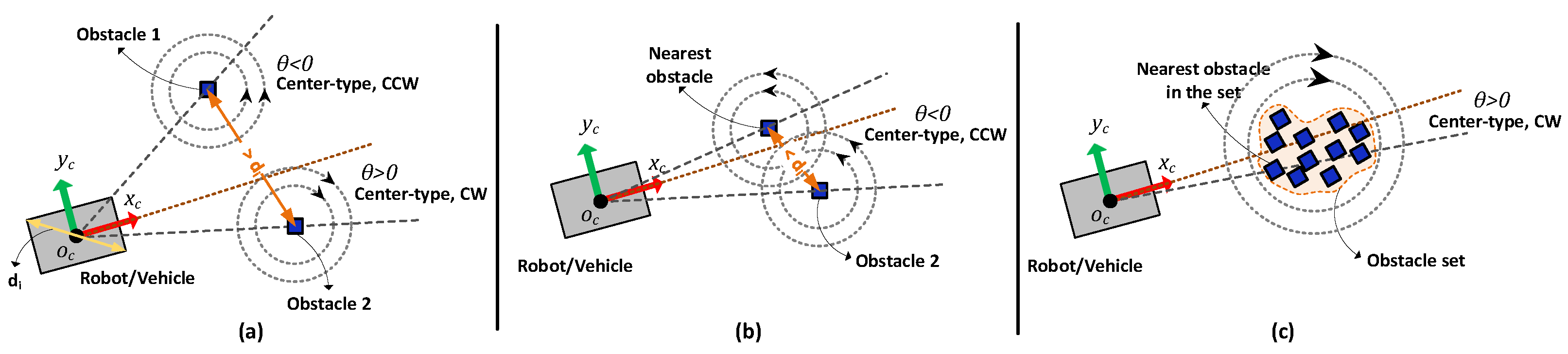
In
Figure 1, the procedure for determining the direction of center-type equilibrium defined at the obstacle position is given. The direction of the equilibrium point is determined depending on the angle
between the instantaneous orientation of the robot/vehicle and the vector drawn from the center of the robot/vehicle to the center of the obstacle. The aim here is to pass the obstacle from the side where the vehicle is headed.
This procedure can only be applied to a single obstacle case. However, in a real-world case, there will be many obstacles in the environment. For this reason, evaluating each obstacle individually may cause confusion. In order to achieve better results, the relative positions of the obstacles should also be noted.
2.5.2. Impact of Multiple Obstacles on the Route Planning
The next waypoint computation uses the expression given in Equation (4) for obstacle-free regions. However, this equation must be modified to include the impact of obstacles on finding the future waypoints. There are two determining factors here: which side the obstacles will direct the path, and the other is the magnitude of this impact.
Here in
Figure 2, the direction determination approach for center-type equilibrium points around obstacles is explained over possible obstacle configurations in an environment. If two separate obstacles are detected in the environment, it is checked whether the distance between the obstacles is wide enough for the robot/vehicle to pass. If there is enough distance between the obstacles (see
Figure 2a), these obstacles are evaluated independently, and direction assignment is made as in the single obstacle case. On the other hand, if they are too close to each other (see
Figure 2b), then the direction is assigned according to the nearest obstacle to the robot/vehicle, and this direction applies to both obstacles. A similar idea can be extended for the multi-obstacle case, where the obstacles are close to each other (see
Figure 2c).
2.6. Overall Path-Finding Process
The instantaneous direction of the path can be achieved using not only the effects of the target but also the impacts of the obstacles and initial pose. In the obstacle-free region case, the effect of the target pose has been examined; here, we have added a ‘
t’ subscript to indicate the target-related effects on the path.
The movement direction from the
kth waypoint (
) is normalized to obtain unit vector
. Similarly, the ‘
i’ subscript is introduced to represent the influence of the initial pose.
Similar to target and initial poses, the impact of a single obstacle (
ith obstacle),
, is computed with Equation (
7)
where
represents the current position of the obstacle and
is unit vector correspondence of
.
,
, and
are two-dimensional square matrices constructed for the stable node equilibrium point at the target pose, unstable node equilibrium point at the initial pose, and center-type equilibrium point at
ith obstacle, respectively. To compute
and
, the definition in Equation (
2) is utilized. On the other hand
relation is used to determine the impact of an obstacle on the path. The total impact of the obstacles is executed with
expression where
represents the number of obstacles detected by the vehicle/robot in step
. Another important point here is that the robot/vehicle may not have prior map knowledge; hence, obstacle detection may rely solely on onboard sensing. To reflect this, only the obstacles located within a predefined sensing radius can be considered in the path calculation. We denote this sensing radius by
R, which determines the maximum distance at which an obstacle can affect the path. In practice,
R corresponds to the effective range of the robot’s obstacle detection sensors.
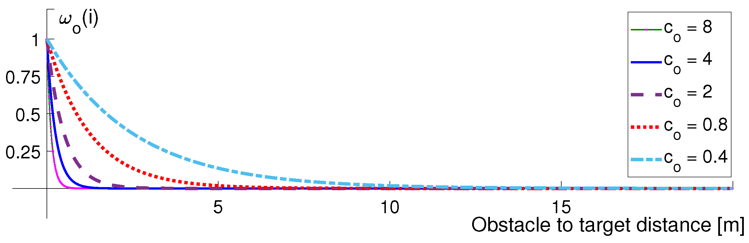
The effect of an obstacle on the path should vary inversely proportional to the distance between the obstacle and the current pose of the robot/vehicle. In order to include this rate, a weight coefficient
is injected to the expression in Equation (
9). Here,
is computed with an exponential expression of Equation (
10).
where
and
describe the decay rate coefficient of an obstacle weight and the inflation radius term, respectively. For the given vehicle/robot in
Figure 2, the inflation radius is
. On the other hand, the
weight profile according to the
constant selection is shown in
Figure 3. When
is selected to be lower, obstacles in remote regions will also affect the direction of the path. However, higher
selection may lead to regulating the robot/vehicle path later, which may cause longer paths. The choice of the coefficient
is important, as it directly influences how strongly obstacles affect the direction of the path based on their distance. A practical selection strategy is to set
relative to the robot’s typical obstacle avoidance range. Specifically, we define
where
is a user-defined sensing or safety radius, and
is a tuning factor (typically between 3 and 6) that controls how sharply the weight decays with distance. This ensures that obstacles beyond the radius
have negligible effect, while those closer influence the path direction significantly. The value of
can be selected based on empirical trials or system responsiveness requirements. In practice, this approach allows
to adapt proportionally to the robot’s sensing capabilities or mission-specific safety margins.
After defining the change in the direction of movement concerning the target pose, initial pose, and surrounding obstacles, the overall movement direction of the path can be computed as in Equation (
11).
where
,
, and
represent the adaptive weights associated with the target pose, initial pose, and obstacles, respectively. These weights satisfy the condition
at each iteration
k. The obstacle weight
is computed as the average influence of the obstacles within sensing range, given by Equation (
12).
Let
be the normalized progress ratio from the initial pose
to the target pose
. Then, the individual weights are defined as follows:
This strategy ensures that the initial orientation initially influences the path, gradually shifts focus to the target pose, and continuously adapts to nearby obstacles throughout the trajectory. Now, the next waypoint of the path can be achieved via the
relation. It is important to note here that in dense environments with multiple nearby obstacles (i.e., obstacle clusters), the interaction of several center-type fields can potentially cause oscillatory or ambiguous path behavior. This occurs when the robot is influenced by several obstacles with similar strengths and directions. Our method mitigates this risk through the use of the weighted vector summation in Equation (
9), where the contribution of each obstacle is modulated by an exponential decay function of distance in Equation (
10). This prioritizes closer or more immediate obstacles and suppresses distant influences, enhancing directional decisiveness. Furthermore, the attractive stable-node field centered at the target ensures global convergence, counteracting local rotational ambiguities. Future versions may incorporate adaptive weights or field saturation models to improve stability in highly cluttered scenes.
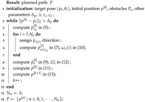
Until now, the mathematical description of the path-finding process is given. In order to see the entire steps of the path-finding process in a compact form, these steps are gathered in Algorithm 1. The algorithm takes the target pose and initial pose information in addition to obstacles detected, and finds the path depending on some parameters such as step size
, target equilibrium eigenvalues
, inflation radius
, and obstacle weight decay rate coefficient
.
| Algorithm 1: Pseudo-code of path-finding approach developed based on phase portrait phenomenon |
![Inventions 10 00065 i001]() |
Here, the generated path P includes the elements for where stands for the number of waypoints on the path. Similarly, the obstacle set includes all the obstacles detected by the vehicle/robot. The working principle of the path-finding algorithm will be illustrated through some basic cases.
2.7. Visual Proof and Explanation of the Concept
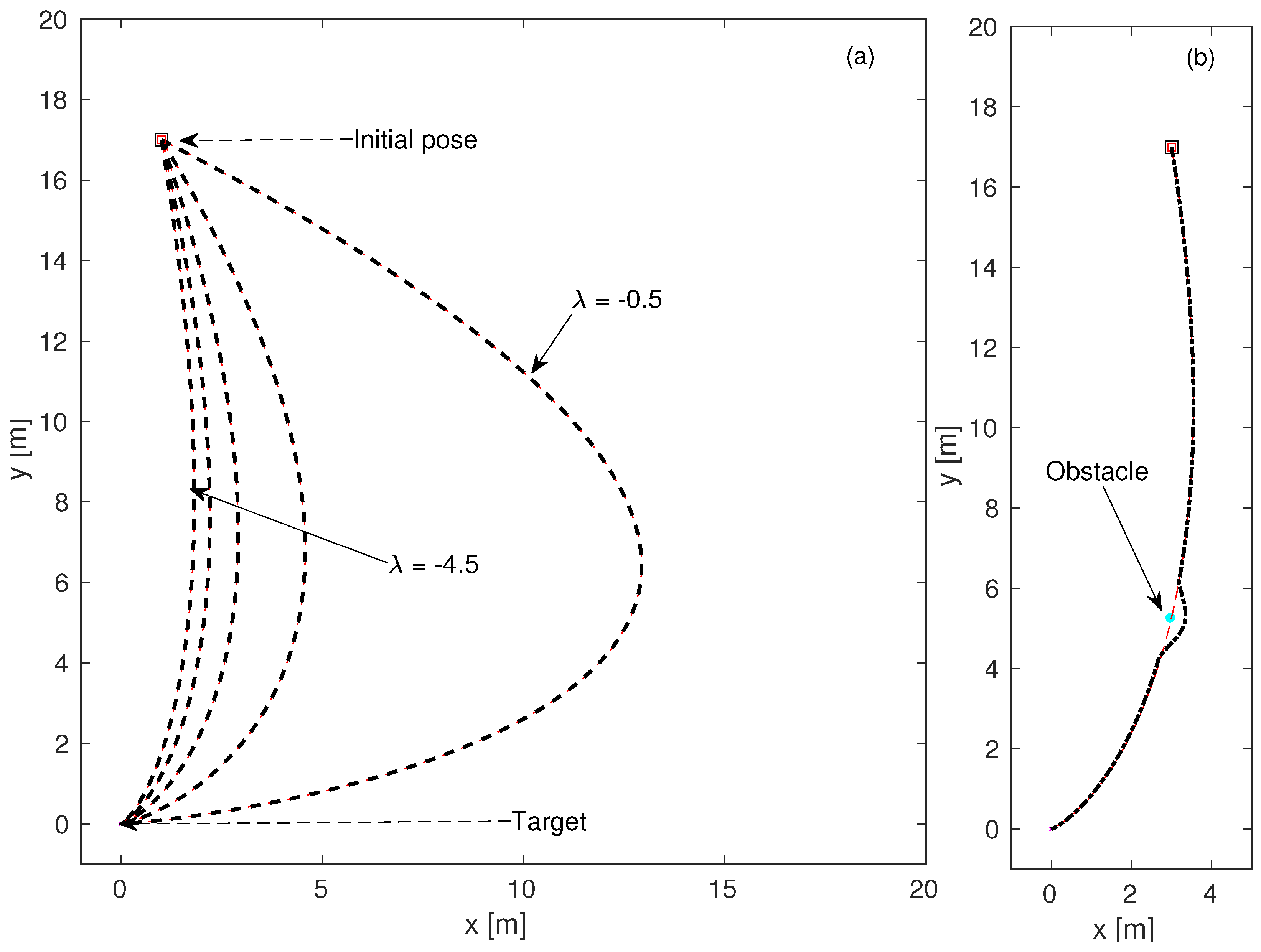
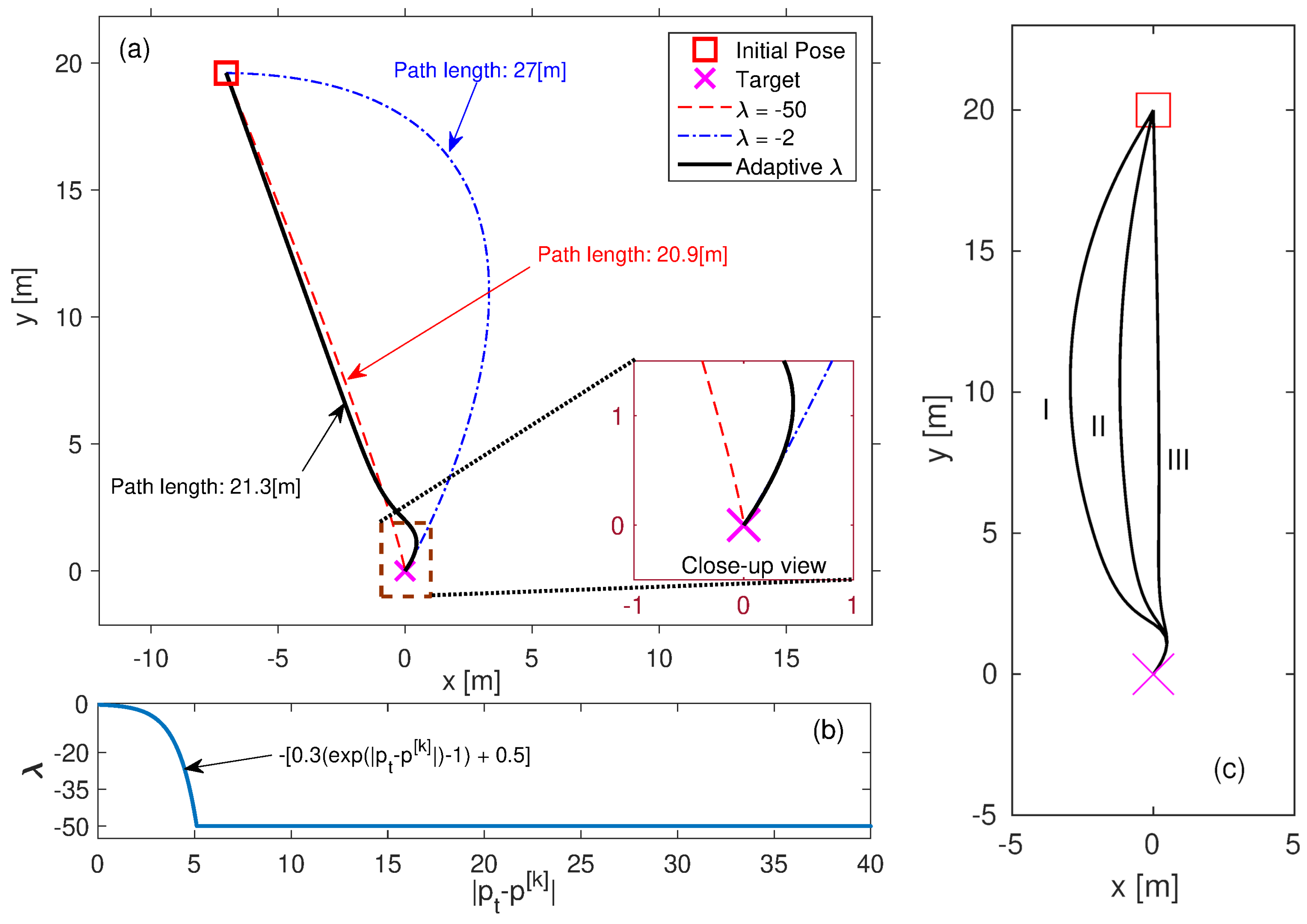
As shown in
Figure 4a, the amplitude of the eigenvalue assigned to the target pose determines the maneuvring radius of the planned path, and a smaller eigenvalue amplitude results in a larger maneuvring radius. Increasing the maneuvre radius eases the approach to the target at the desired orientation, but keeping the maneuvre radius large along the entire route may result in unnecessarily longer routes.
When an obstacle blocks the path, the algorithm proposed in this study updates the path accordingly, considering the effects of equilibrium points defined at both the obstacle position and the target position (see
Figure 4b).
The problem shown in
Figure 4a can be overcome by selecting the amplitude of the assigned eigenvalue high initially and decreasing it adaptively as the vehicle/robot approaches the target over time, since the aim is to both reach the target with desired orientation and make the route as short as possible (see in
Figure 5a). In the adaptive case, the
is tuned between −50 and −0.5 with respect to the current distance to the target pose as shown in
Figure 5b. The initial orientation of the robot/vehicle can also be considered while generating the path as demonstrated in
Figure 5c. Similar to the target, the eigenvalues are adaptively assigned for the initial pose, such that
and there is a span between 0.5 and 50 as the vehicle/robot moves away from the initial pose.
In
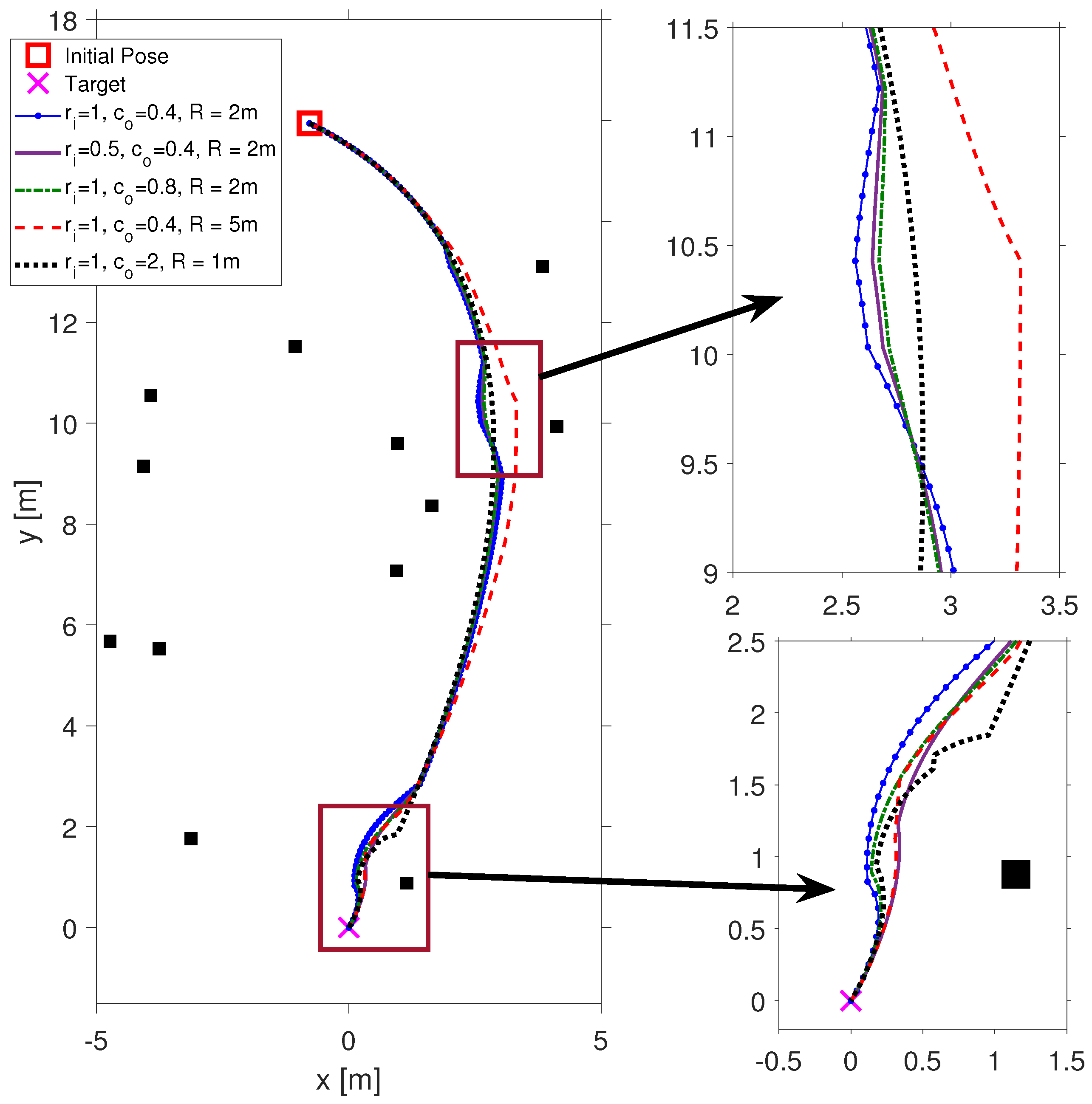
Figure 4b, the single obstacle case for path-finding is investigated. However, in a real-world scenario, it is likely to have many more obstacles around it. The path-finding result of our algorithm for the multi-obstacle case is demonstrated in
Figure 6. The parameters
, the eigenvalue pair of the stable node equilibrium point defined at the target pose, and
, the distance between consecutive waypoints, are kept constant. On the other hand, the deviation on the path is examined in five separate trials with respect to inflation radius
, obstacle weight decay rate coefficient
, and the range at which the algorithm begins to consider obstacles
R parameters. As shown in
Figure 6, increasing the inflation radius
or the obstacle weight decay coefficient
leads to earlier and stronger reactions to nearby obstacles, resulting in more pronounced path deviations around them. On the other hand, reducing the sensor range
R limits obstacle awareness, causing the vehicle to respond later to potential collisions, which may increase the risk of close encounters or inefficient detours. These experiments demonstrate the trade-off between safety margin, reactivity, and path efficiency. The selection of these parameters should therefore consider the robot’s sensing capabilities and operating environment.
2.8. Conceptual Comparison with Existing Path-Finding Algorithms
While the quantitative comparisons will be demonstrated in the next section, it is also important to discuss the methodological distinctions between our approach and other widely used planning algorithms in autonomous robots/vehicles.
A* and Hybrid A*: A* is a grid-based graph search algorithm that computes the shortest path using a heuristic cost function but does not account for vehicle orientation. Hybrid A*, on the other hand, incorporates orientation and motion constraints by allowing non-holonomic transitions between states. However, it tends to be computationally expensive; in contrast, our planner continuously integrates both positional and orientation objectives through phase portrait dynamics, offering orientation-aware paths with lower computational requirements.
RRT and RRT* These are sampling-based planners that generate random trees to explore the configuration space. While they are effective in complex environments, they often produce jerky, sub-optimal paths that require post-processing. They also do not inherently consider final orientation or system dynamics unless extended variants are used. The proposed method inherently produces smooth and dynamically feasible paths due to the continuous nature of the differential equations used.
Costmap Requirement: A* and RRT-based methods require an inflated map (costmap) to account for the robot’s physical dimensions. The proposed method, however, incorporates an inflation radius parameter directly into the path computation, eliminating the need for external preprocessing and reducing memory requirements.
Planning Model: Unlike discrete planners, our algorithm exploits continuous vector field integration, allowing both global and local planning without reinitialization or heavy sampling.
In summary, our planner combines the benefits of orientation-aware planning (like Hybrid A*) with continuous dynamics and low memory overhead and offers a favorable trade-off between efficiency, feasibility, and implementation simplicity.
3. Results
The simulation experiments are conducted using the MATLAB software (release 2020b). In the path-finding process, only obstacles within the forward field of view are considered, since obstacles located behind the robot do not influence forward motion planning. To reflect this, a field of view of ±60° is applied relative to the robot’s local coordinate frame and any obstacles outside this angular range are disregarded.
To evaluate the performance of the proposed planner under different conditions, 28 separate path-finding simulations are performed to follow the practice in motion planning benchmarking [
30], each corresponding to a unique navigation scenario defined by different combinations of initial and target positions and orientations. These simulations cover nine representative test cases with repeated runs to ensure statistical validity across two different map environments: an indoor map, designed to simulate narrow and constrained pathways, and the playpen map, which contains open areas with clustered obstacles. This setup allows for a comprehensive and fair comparison across planning algorithms in terms of path length, smoothness, orientation accuracy, and computational efficiency.
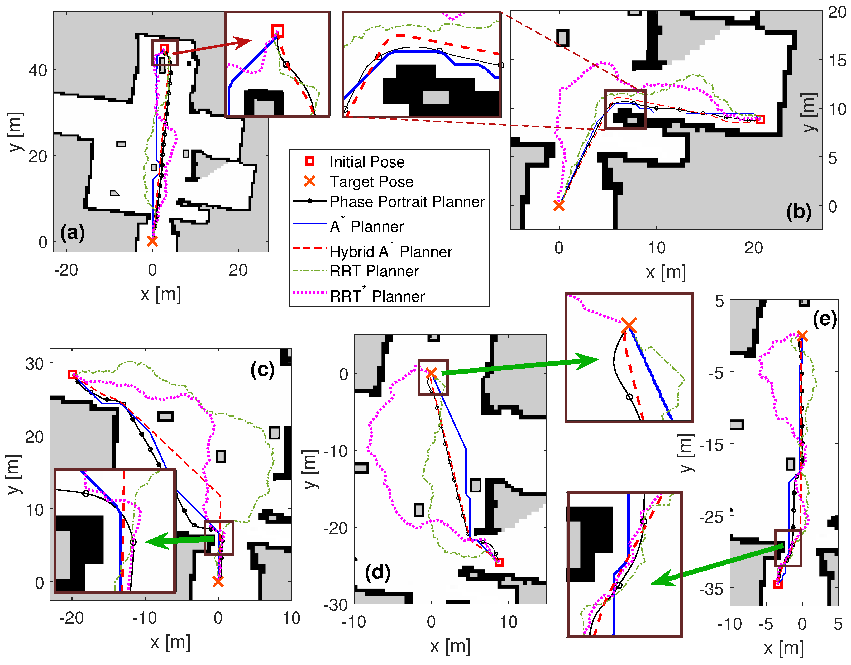
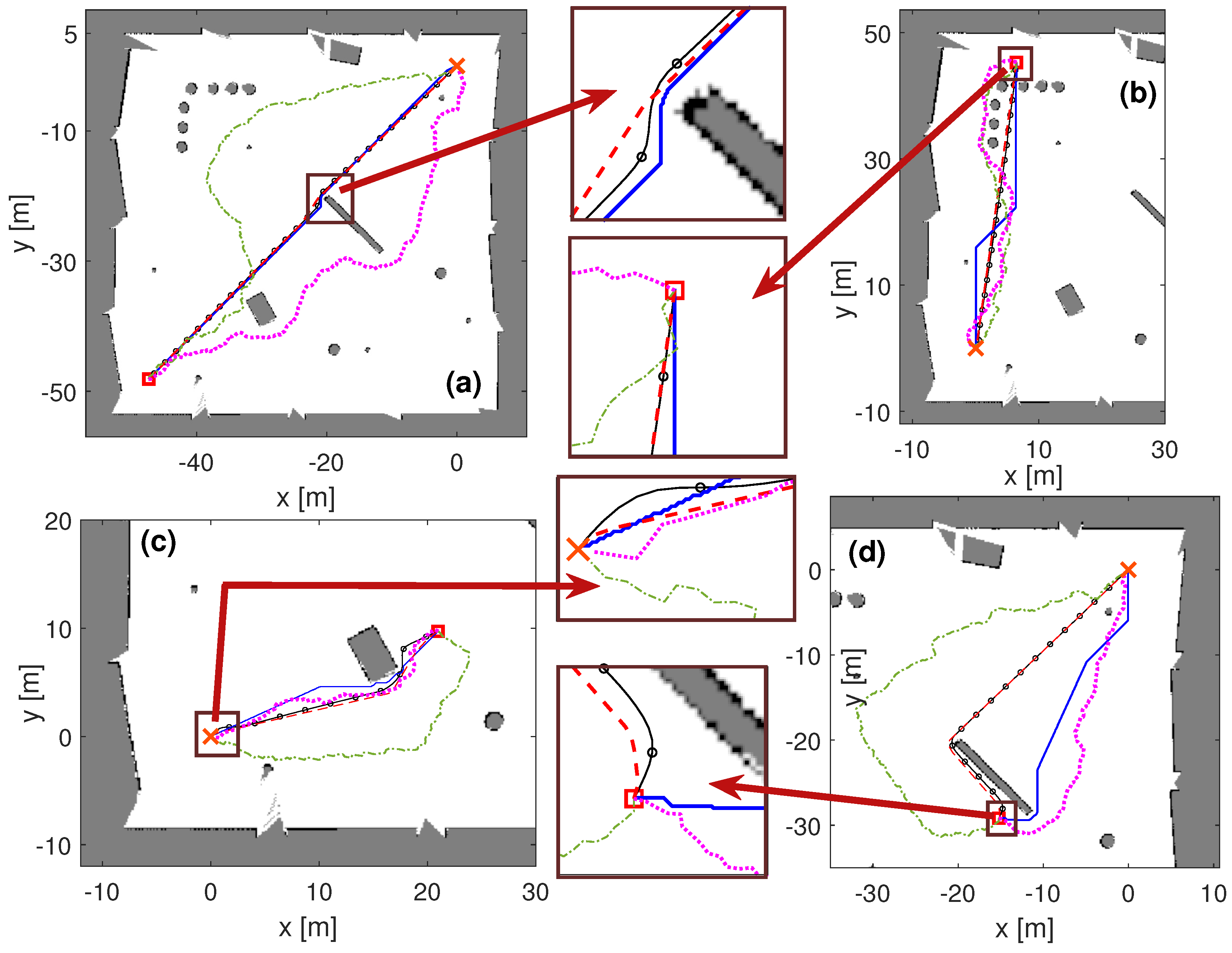
The results of these simulations are illustrated in
Figure 7 and
Figure 8, which show the path-finding results of the proposed algorithm alongside several state-of-the-art planners across the nine test cases. The path slices around obstacles and/or target poses have been highlighted with the close-up views to indicate that our algorithm passes through obstacles by planning a smooth path and guarantees docking to the target with the desired orientation.
According to the quantitative results in
Table 1, the proposed phase portrait planner and Hybrid A* methods are orientation-aware planners, their orientation errors are zero, and they have found the shortest paths. However, Hybrid A* has the longest planning times in both scenarios. The phase portrait planner method is close to Hybrid A* in path length; however, it has a shorter planning time. It presents an improvement of 58.32s and 71.67s (84% (indoor map) and 52% (playpen map)) in planning time compared to the Hybrid A* algorithms, respectively.
To evaluate the robustness and scalability of the proposed planner, a systematic comparison was conducted across different obstacle densities (0%—obstacle free, 5%, 10%, and 20%).
Table 2 summarizes the path length and computation time for five common planning algorithms. The results demonstrate that our method maintains a smooth and consistent increase in path length as obstacle density rises, with a growth of approximately 82% from 35.9 m to 65.4 m. In terms of computation time, our method scales predictably from 0.087 s to 4.12 s—remaining within the bounds of real-time feasibility. In contrast, Hybrid A* shows severe scalability issues, increasing from 0.206 s to 86.1 s as density increases. Although A* remains fast, it requires a separate inflation phase and does not consider the final orientation of the vehicle/robot. Sampling-based methods (RRT and RRT*) exhibit variable performance due to their sampling-based probabilistic nature. These findings underscore the robustness and efficiency of our method in cluttered maps without relying on map inflation and support its applicability in complex scenarios.
Other approaches simulated in this study do not avoid or find a collision-free path by considering vehicle dimensions. To achieve this tolerance, the inflated version of the map (costmap) must be supplied. However, the advantage of the proposed algorithm is that it does not require an inflated map, as the inflation radius parameter is already evaluated in the path-finding procedure. This also makes the proposed algorithm a cost-effective solution in terms of memory requirements. As a result, these simulation experiments validated the merits of the proposed system.
4. Conclusions
Orientation-aware path planning algorithms search for not only the shorter path from the initial to the target position but also take into account the orientation of the target location, initial orientation, and the obstacles in the environment to build a smooth and collision-free path for robots with non-holonomic constraints. In this study, we adopt a widely used behavioral analysis technique of nonlinear systems, known as the phase portrait phenomenon, as an orientation-aware path-finding algorithm that can be used both as a global and online planner in continuous search space.
The effectiveness of the proposed method has been demonstrated through various simulation scenarios and against state-of-the-art approaches such as A*, Hybrid A*, RRT, and RRT*. The results show that our method achieves zero orientation error, competitive or shorter path lengths, and significantly faster planning times with up to 84% reduction in computation time compared to Hybrid A*. The significance of this study can be well recognized in mission-critical applications involving non-holonomic mobile robots operating in continuous space, where trajectory length, path feasibility, and precise final orientation, such as for docking, are essential.
In future studies, the proposed method will be tested on real robotic platforms to further validate the method’s applicability and robustness level against sensor noise, actuation inaccuracies, localization errors, and dynamic obstacles. Although our approach is formulated to support online planning based on local perception, the current evaluation is limited to static environments to provide fair and comparable results with existing algorithms. Future work will extend the method to address moving obstacles explicitly. We also aim to extend the approach to three-dimensional (3D) environments. As discussed in the ’Qualitative Features’ chapter of the ‘
Nonlinear Dynamics’ book [
31], an n-dimensional phase space can be constructed using coordinates
. To extend the proposed 2D method to 3D path planning, the same phase portrait-based framework can be adapted by generalizing the state vector and system dynamics. In 3D space, the position vector becomes
, and the corresponding system dynamics can be modeled using a 3 × 3 matrix
A such that
, where
is the target position. The eigenstructure of matrix
A can be designed to ensure a stable node equilibrium at the target pose with user-defined final orientation, similar to the 2D case but now represented by a 3D unit vector or quaternion. Obstacles can also be represented as center-type equilibrium points using skew-symmetric matrices that define rotational fields around each obstacle. This extension enables the planner to account for motion constraints in 3D environments, effectively update paths in response to newly detected obstacles, and supports applications in aerial robotics or underwater navigation, such as drones, aircraft, and submarines.


