
Optimization of Passenger Train Line Planning Adjustments Based on Minimizing Systematic Costs


Abstract
1. Introduction
- A systematic cost metric is proposed for train line planning optimization, enabling a comprehensive assessment of optimization performance. In addition, optimization trigger mechanisms are designed to determine when updates to the line plan are necessary, thereby supporting smoother and more adaptive transportation operations.
- Line planning is optimized based on train routing, ensuring both the feasibility of train deployment and the operational stability of the resulting plan.
- A neighborhood search strategy is developed to jointly optimize individual train routes and the overall line plan, achieving coordination between localized routing decisions and system-level operational efficiency.
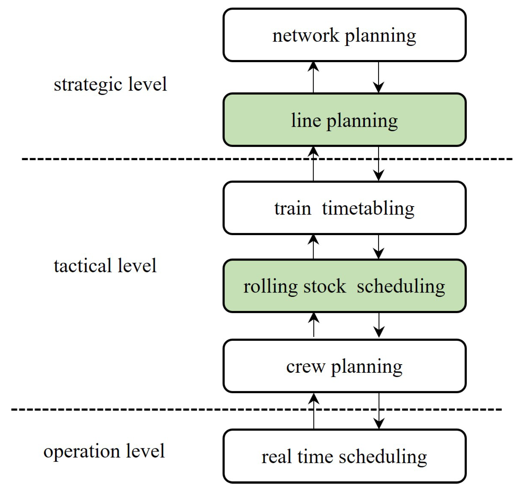
2. Methods
2.1. Problem Description
- Each train has an optimized routing path, stop pattern, formation type, and departure/arrival times;
- The passenger flow is reasonably assigned to the available travel plans;
- The resource constraints, such as track capacity and time windows, are satisfied.
2.2. Notations
2.3. Systematic Costs
2.3.1. Components of Train Operations
- Train Operation
- Energy Consumption
- Passenger Services
2.3.2. Cost Components of Passenger Travel
- Travel Adjustment Costs
- Travel Plan Costs
- Balanced Stop Costs
- Systematic Costs
2.4. Passenger Train Line Planning Optimization Model
2.4.1. Trigger Criteria Design for Passenger Train Line Planning Optimization
- Passenger Flow Demand Fluctuation
- Change in Load Factor
2.4.2. Constraints
- Transportation Resource Constraints
- Transportation Organization Constraints
- Service Level Constraints
- Train Capacity Constraints
2.4.3. Objective Function
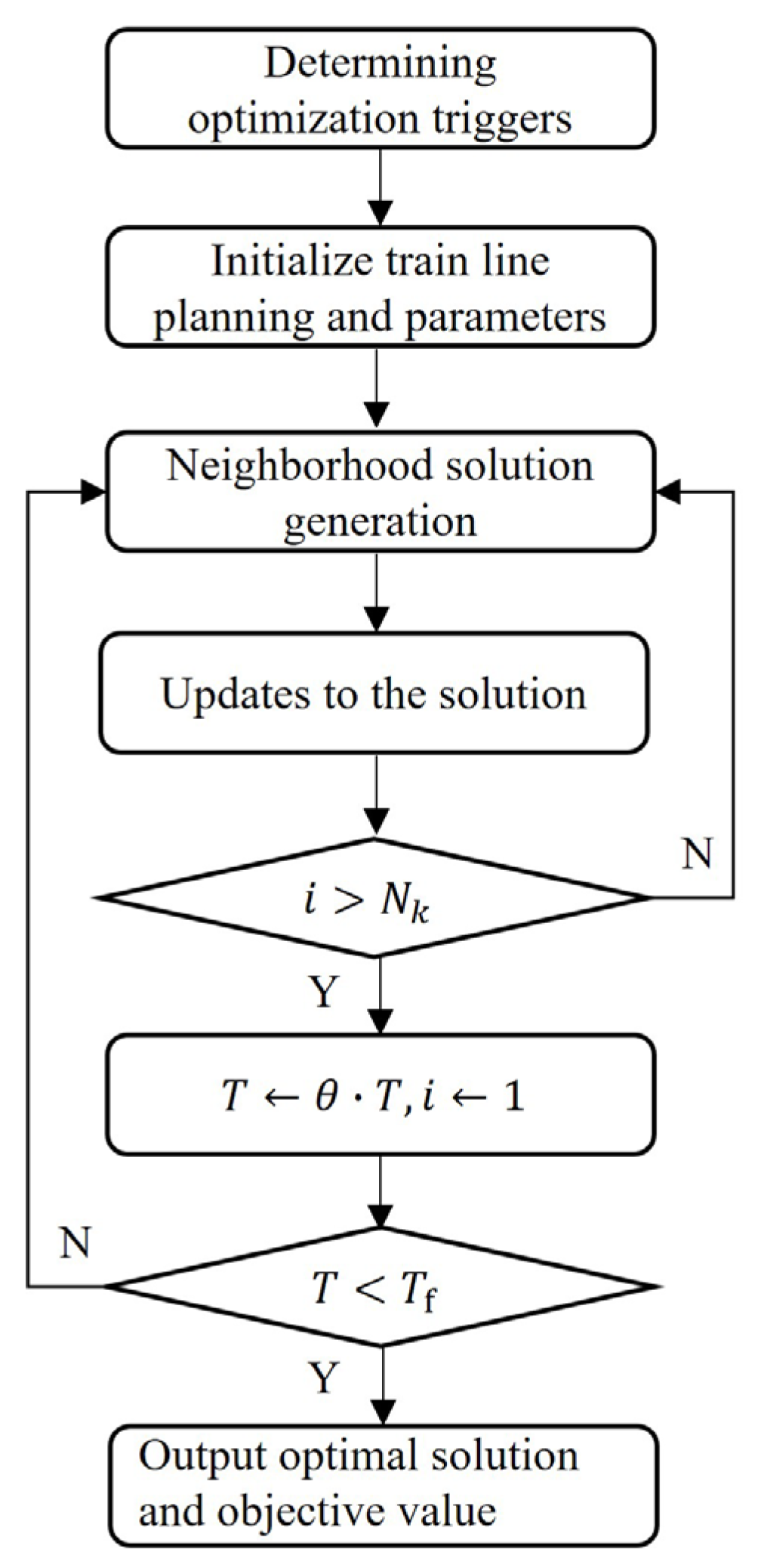
2.5. Algorithm
2.5.1. Optimization Strategy
- Adjustment Optimization Trigger Determination
- Initial Solution Construction and Evaluation
- Solution Update
- Termination Condition Check
2.5.2. Neighborhood Search Strategy
- Route Train Adjustment Strategy
- Overall Adjustment Strategy for the Plan
2.5.3. Algorithm Process
3. Results and Discussion
3.1. Parameter Settings
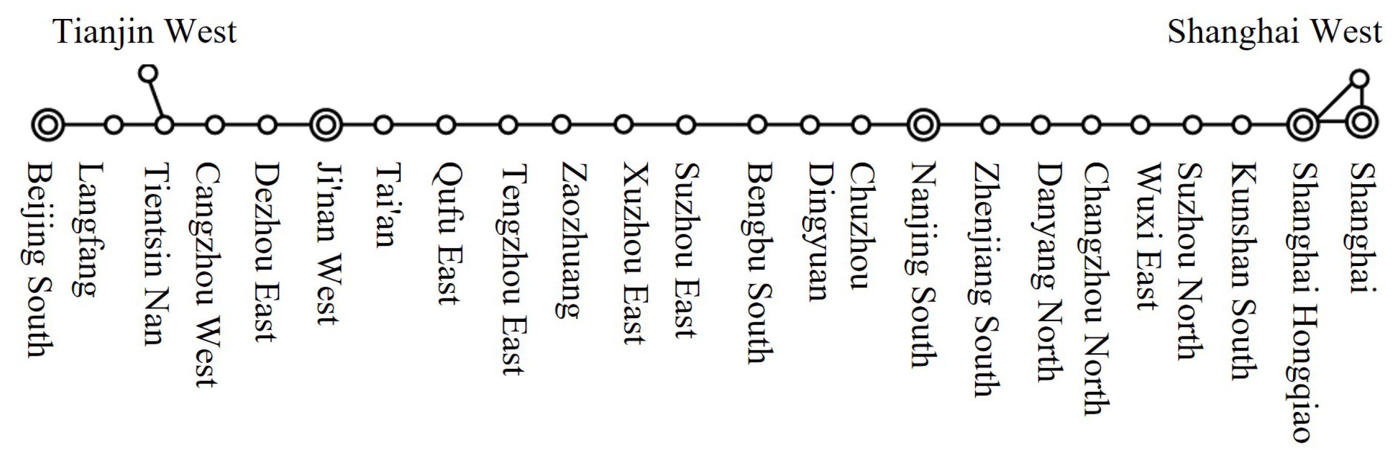
3.1.1. High-Speed Rail Network and Train Data
3.1.2. Passenger Flow Demand Data
3.1.3. Cost Parameter Settings
- Track Usage Fee Parameters
- Contact Network Usage Fee Parameters
- Station Passenger Service Fee Parameters
- Ticketing Service Fee Parameters
- Station Water Supply Service Fee Parameters
- Passenger Travel Cost Parameters
3.1.4. Other Parameters
3.2. Result Analysis
3.2.1. Adjustment and Optimization Trigger Judgment
- Passenger Demand Fluctuation
- Seat Occupancy Changes
3.2.2. Optimization Results Analysis
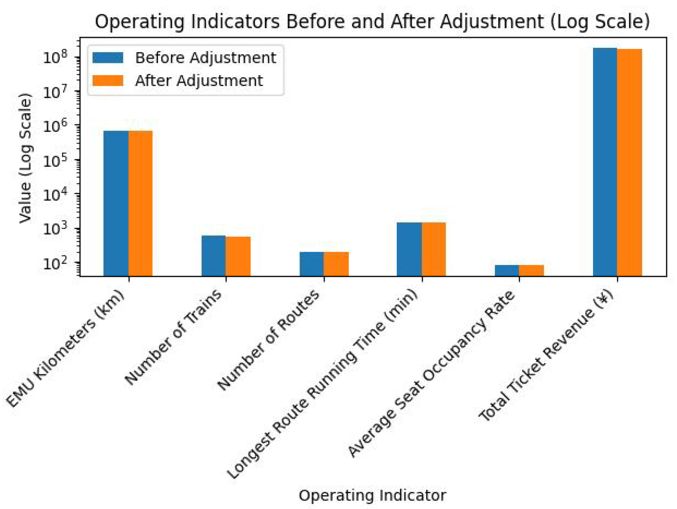
- Operating Indicator Analysis
- (1)
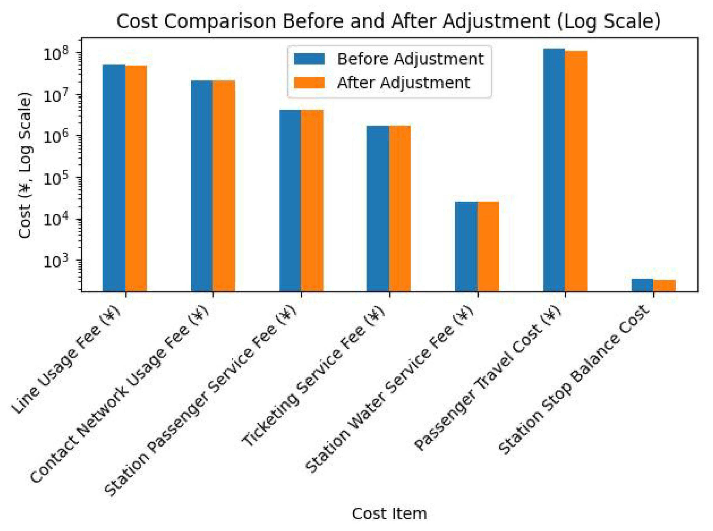
- Comparison of Operating Indicators Before and After Adjustment
- (2)
- Train Seat Occupancy Rate
- (3)
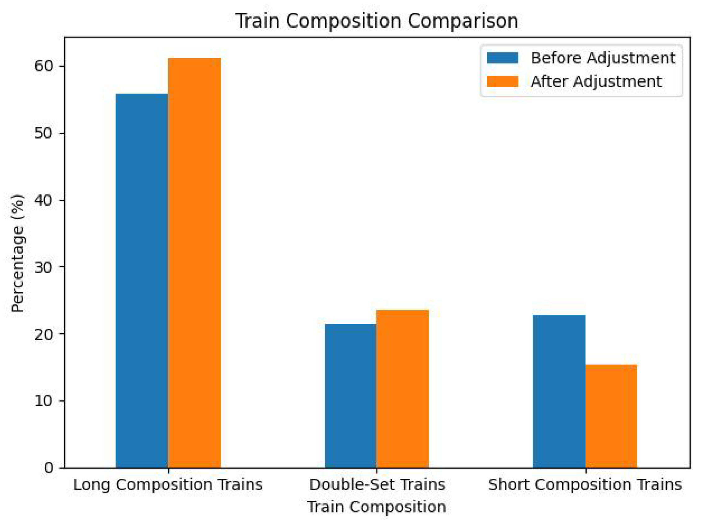
- Train Composition
- (4)
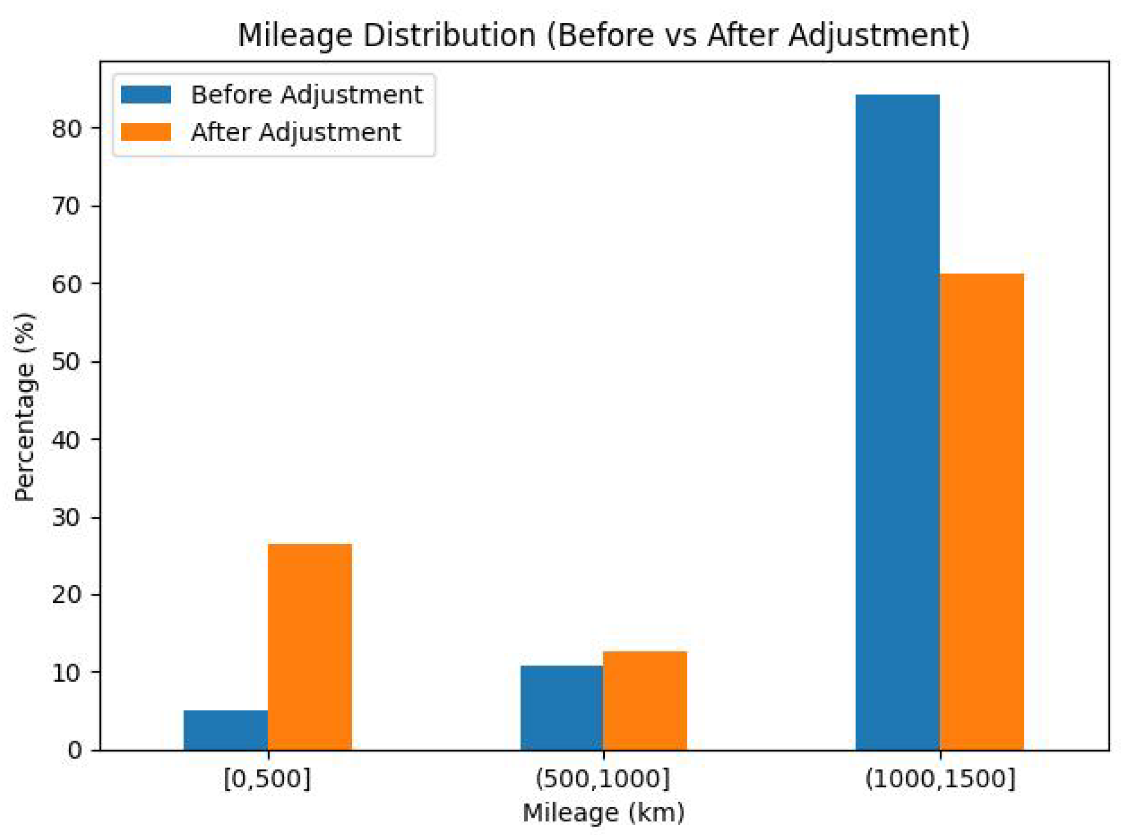
- Train Operation Distance
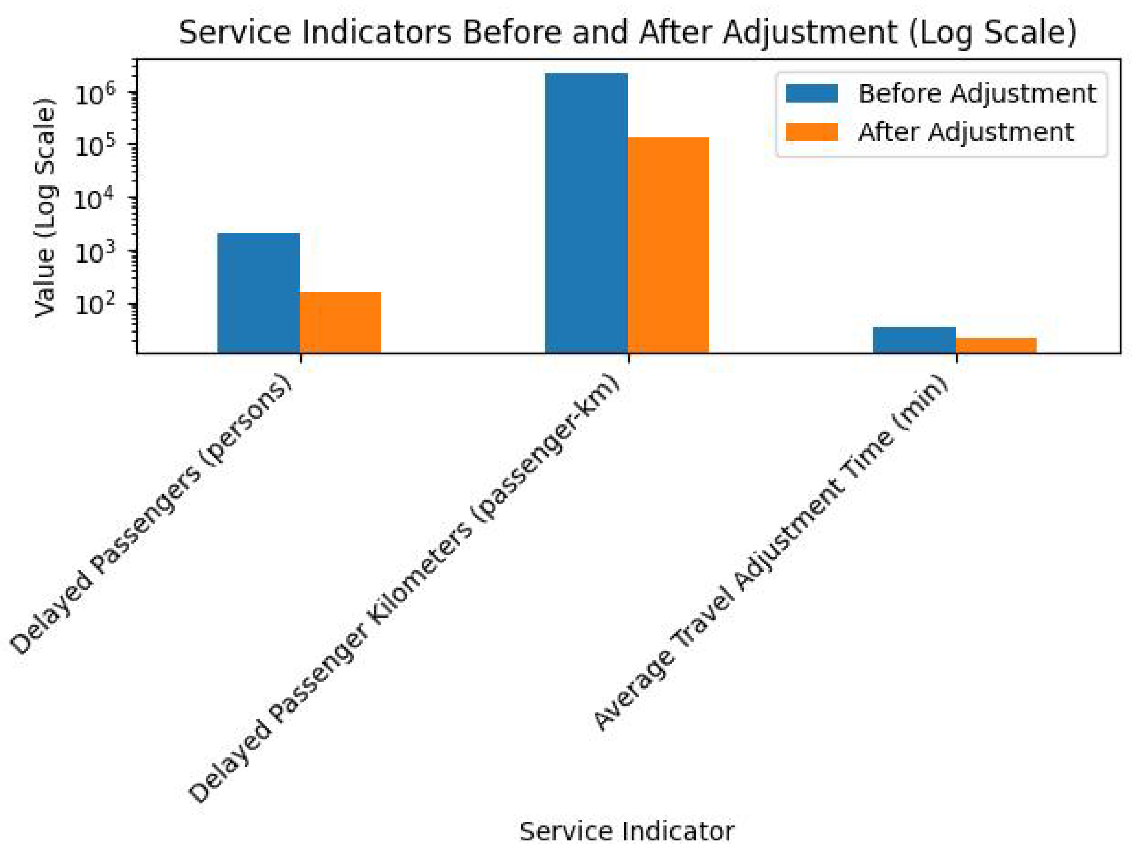
- Service Indicators Analysis
- (1)
- Service Indicator Comparison Before and After Adjustment
- (2)
- Delayed Passenger Flow
- (3)
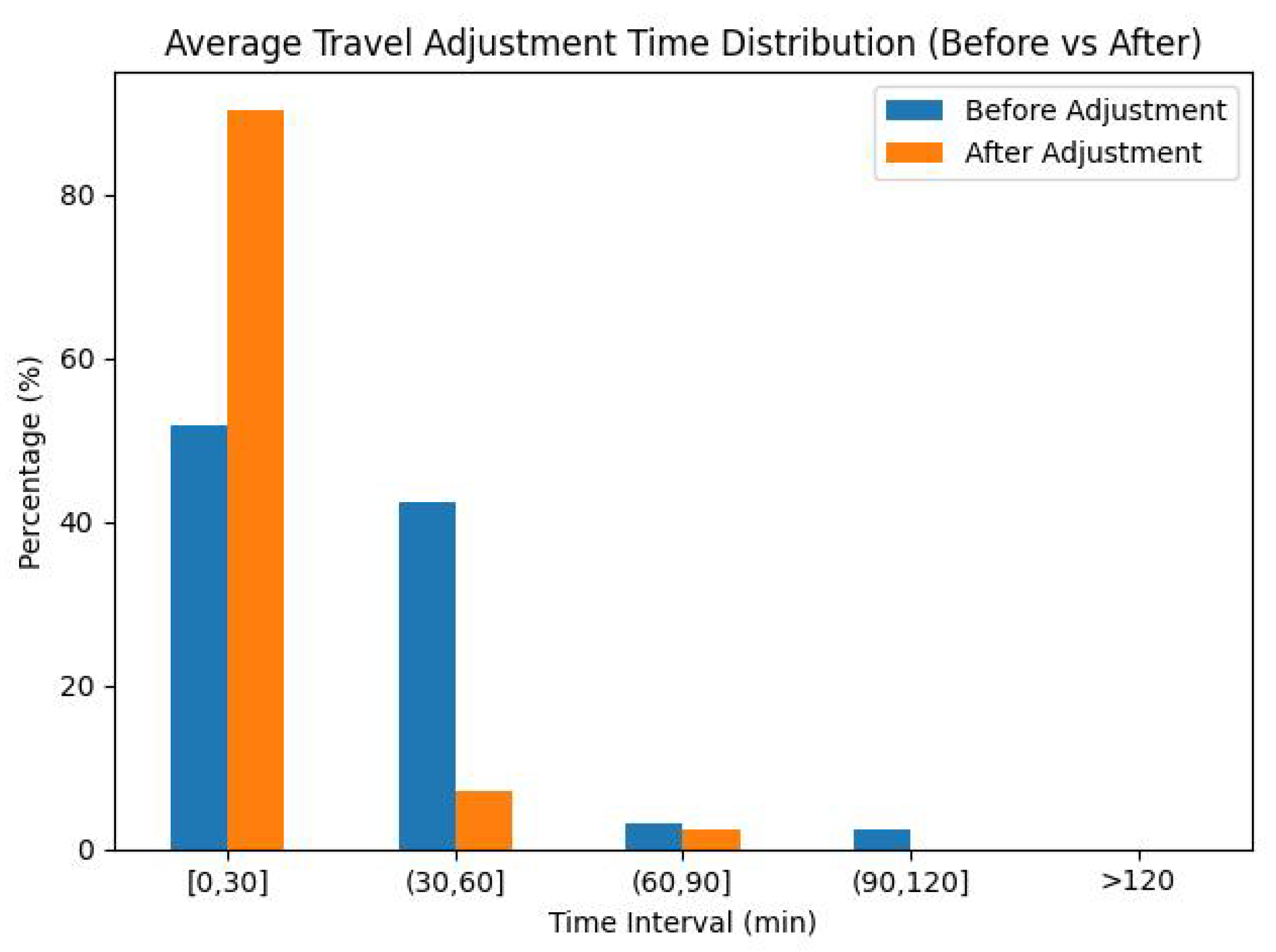
- Travel Adjustment Time
- (4)
- Train Stop Ratio
- (5)
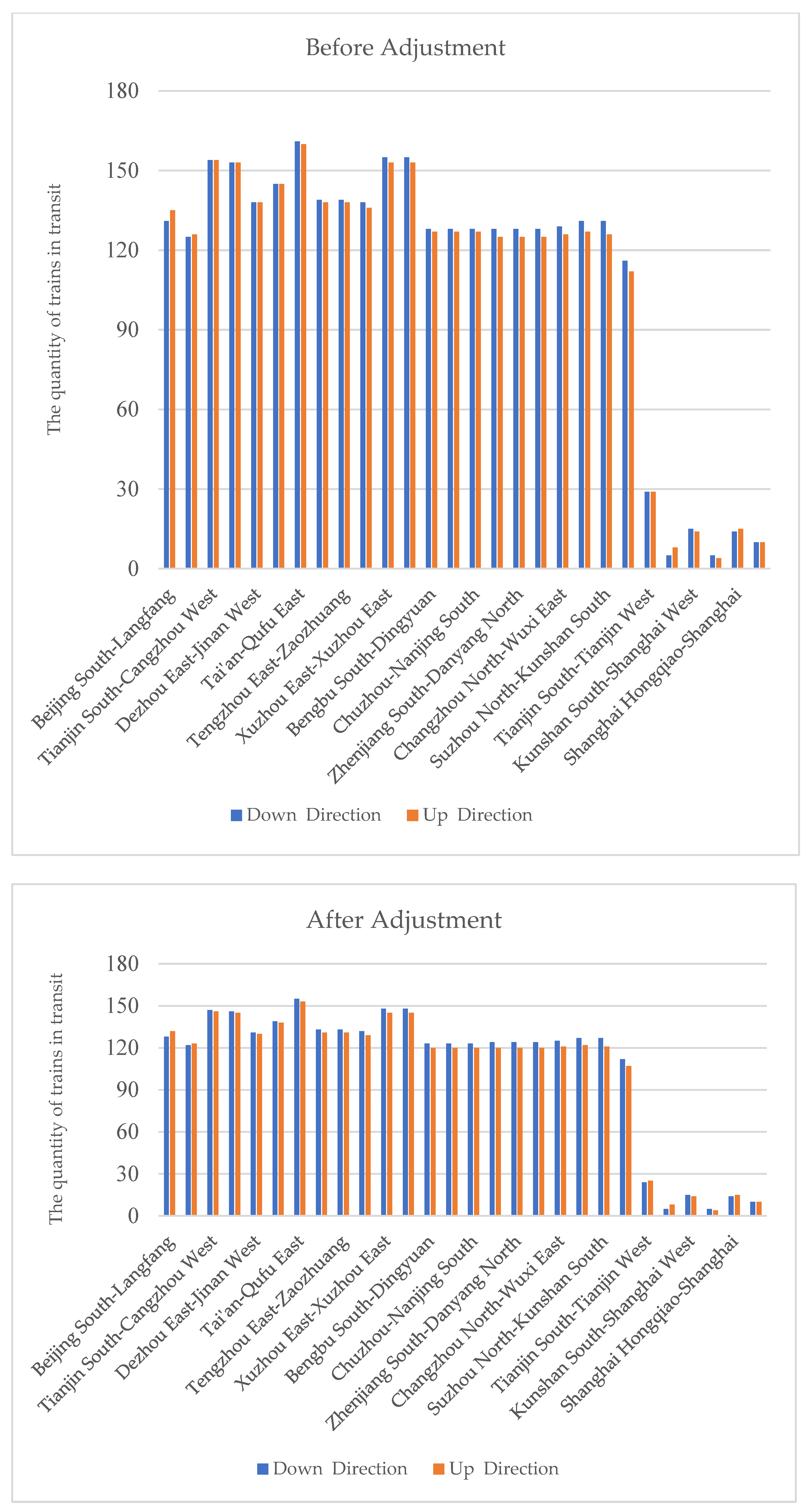
- Station Service Frequency
- Analysis of Capacity Resource Utilization
- (1)
- Utilization of Station Departure and Arrival Capacity
- (2)
- Utilization of Section Throughput Capacity
- (3)
- Utilization of EMU Fleet Resources
- Comparison with Actual Plan
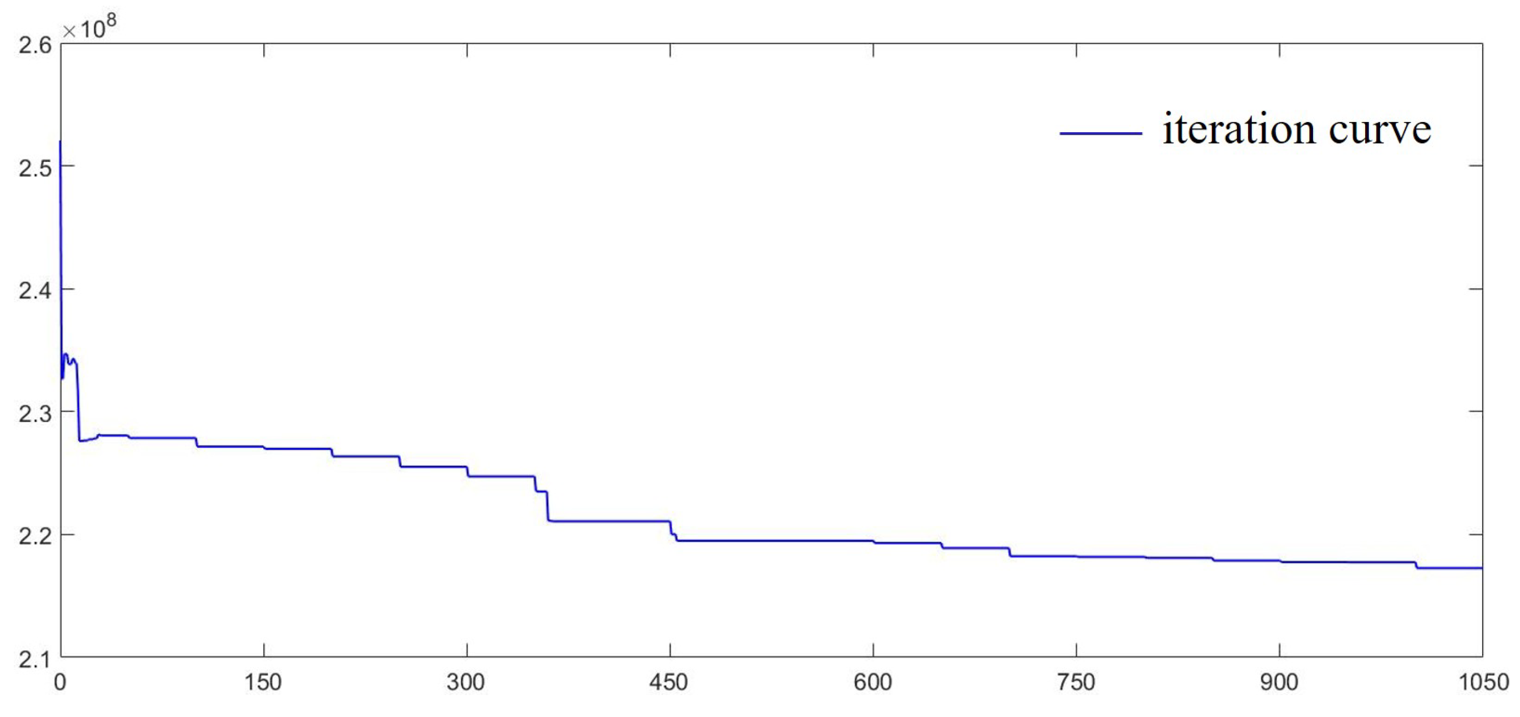
3.2.3. Sensitivity Analysis
4. Conclusions
Author Contributions
Funding
Institutional Review Board Statement
Informed Consent Statement
Data Availability Statement
Conflicts of Interest
References
- Lusby, R.M.; Larsen, J.; Ehrgott, M.; Ryan, D. Railway track allocation: Models and methods. OR Spectr. 2011, 33, 843–883. [Google Scholar] [CrossRef]
- Canca, D.; De-Los-Santos, A.; Laporte, G.; Mesa, J.A. An adaptive neighborhood search metaheuristic for the integrated railway rapid transit network design and line planning problem. Comput. Oper. Res. 2017, 78, 1–14. [Google Scholar] [CrossRef]
- Cacchiani, V.; Qi, J.; Yang, L. Robust optimization models for integrated train stop planning and timetabling with passenger demand uncertainty. Transp. Res. Part B: Methodol. 2020, 136, 1–29. [Google Scholar] [CrossRef]
- Talebian, A.; Zou, B. Integrated modeling of high performance passenger and freight train planning on shared-use corridors in the US. Transp. Res. Part B Methodol. 2015, 82, 114–140. [Google Scholar] [CrossRef]
- Polinder, G.-J.; Schmidt, M.; Huisman, D. Timetabling for strategic passenger railway planning. Transp. Res. Part B Methodol. 2021, 146, 111–135. [Google Scholar] [CrossRef]
- Xu, R.; Wang, F.; Zhou, F. Train stop schedule plan optimization of high-speed railway based on time-segmented passenger flow demand. In Proceedings of the Sixth International Conference on Transportation Engineering, Nanjing, China, 19–20 July 2019; American Society of Civil Engineers: Reston, VA, USA, 2019; pp. 899–906. [Google Scholar]
- Tang, L.; Xu, X. Optimization for operation scheme of express and local trains in suburban rail transit lines based on station classification and bi-level programming. J. Rail Transp. Plan. Manag. 2022, 21, 100283. [Google Scholar] [CrossRef]
- Hai, X.; Zhao, C. Optimization of train working plan based on multiobjective bi-level programming model. J. Inf. Process. Syst. 2018, 14, 487–498. [Google Scholar]
- Yang, Y.; Li, J.; Wen, C.; Huang, P.; Peng, Q.; Lessan, J. A bi-level passenger preference-oriented line planning model for high-speed railway operations. Transp. Res. Rec. 2018, 2672, 224–235. [Google Scholar] [CrossRef]
- Liu, X.; Dabiri, A.; Xun, J.; De Schutter, B. Bi-level model predictive control for metro networks: Integration of timetables, passenger flows, and train speed profiles. Transp. Res. Part E Logist. Transp. Rev. 2023, 180, 103339. [Google Scholar] [CrossRef]
- Zhu, Y.; Mao, B.; Bai, Y.; Chen, S. A bi-level model for single-line rail timetable design with consideration of demand and capacity. Transp. Res. Part C Emerg. Technol. 2017, 85, 211–233. [Google Scholar] [CrossRef]
- Yu, B.; Kong, L.; Sun, Y.; Yao, B.; Gao, Z. A bi-level programming for bus lane network design. Transp. Res. Part C Emerg. Technol. 2015, 55, 310–327. [Google Scholar] [CrossRef]
- Kroon, L.; Maróti, G.; Nielsen, L. Rescheduling of railway rolling stock with dynamic passenger flows. Transp. Sci. 2015, 49, 165–184. [Google Scholar] [CrossRef]
- Cacchiani, V.; Caprara, A.; Galli, L.; Kroon, L.; Maróti, G.; Toth, P. Railway rolling stock planning: Robustness against large disruptions. Transp. Sci. 2012, 46, 217–232. [Google Scholar] [CrossRef]
- Peeters, M.; Kroon, L. Circulation of railway rolling stock: A branch-and-price approach. Comput. Oper. Res. 2008, 35, 538–556. [Google Scholar] [CrossRef]
- Cadarso, L.; Marín, Á. Improving robustness of rolling stock circulations in rapid transit networks. Comput. Oper. Res. 2014, 51, 146–159. [Google Scholar] [CrossRef]
- Alfieri, A.; Groot, R.; Kroon, L.; Schrijver, A. Efficient circulation of railway rolling stock. Transp. Sci. 2006, 40, 378–391. [Google Scholar] [CrossRef]
- Canca, D.; Sabido, M.; Barrena, E. A rolling stock circulation model for railway rapid transit systems. Transp. Res. Procedia 2014, 3, 680–689. [Google Scholar] [CrossRef]
- Canca, D.; Barrena, E. The integrated rolling stock circulation and depot location problem in railway rapid transit systems. Transp. Res. Part E Logist. Transp. Rev. 2018, 109, 115–138. [Google Scholar] [CrossRef]
- Abbink, E.; Berg, B.v.D.; Kroon, L.; Salomon, M. Allocation of railway rolling stock for passenger trains. Transp. Sci. 2004, 38, 33–41. [Google Scholar] [CrossRef]
- Wagenaar, J.; Kroon, L.; Fragkos, I. Rolling stock rescheduling in passenger railway transportation using dead-heading trips and adjusted passenger demand. Transp. Res. Part B Methodol. 2017, 101, 140–161. [Google Scholar] [CrossRef]
- Haahr, J.T.; Wagenaar, J.C.; Veelenturf, L.P.; Kroon, L.G. A comparison of two exact methods for passenger railway rolling stock (re) scheduling. Transp. Res. Part E Logist. Transp. Rev. 2016, 91, 15–32. [Google Scholar] [CrossRef]
- Giacco, G.L.; D’Ariano, A.; Pacciarelli, D. Rolling stock rostering optimization under maintenance constraints. J. Intell. Transp. Syst. 2014, 18, 95–105. [Google Scholar] [CrossRef]
- Hoogervorst, R.; Dollevoet, T.; Maróti, G.; Huisman, D. Reducing passenger delays by rolling stock rescheduling. Transp. Sci. 2020, 54, 762–784. [Google Scholar] [CrossRef]
- Lai, Y.-C.; Fan, D.-C.; Huang, K.-L. Optimizing rolling stock assignment and maintenance plan for passenger railway operations. Comput. Ind. Eng. 2015, 85, 284–295. [Google Scholar] [CrossRef]
- Tréfond, S.; Billionnet, A.; Elloumi, S.; Djellab, H.; Guyon, O. Optimization and simulation for robust railway rolling-stock planning. J. Rail Transp. Plan. Manag. 2017, 7, 33–49. [Google Scholar] [CrossRef]
- Zhao, P.; Li, Y.; Han, B.; Yang, R.; Liu, Z. Integrated optimization of rolling stock scheduling and flexible train formation based on passenger demand for an intercity high-speed railway. Sustainability 2022, 14, 5650. [Google Scholar] [CrossRef]
- Zhao, S.; Yang, H.; Wu, Y. An integrated approach of train scheduling and rolling stock circulation with skip-stopping pattern for urban rail transit lines. Transp. Res. Part C Emerg. Technol. 2021, 128, 103170. [Google Scholar] [CrossRef]
- Wang, Y.; D’aRiano, A.; Yin, J.; Meng, L.; Tang, T.; Ning, B. Passenger demand oriented train scheduling and rolling stock circulation planning for an urban rail transit line. Transp. Res. Part B Methodol. 2018, 118, 193–227. [Google Scholar] [CrossRef]
- Zhou, H.; Qi, J.; Yang, L.; Shi, J.; Pan, H.; Gao, Y. Joint optimization of train timetabling and rolling stock circulation planning: A novel flexible train composition mode. Transp. Res. Part B Methodol. 2022, 162, 352–385. [Google Scholar] [CrossRef]
- Li, C.; Zhang, Q.; Fang, B.; Wei, Y. An optimisation and adjustment model of train line planning for EMU trains under multiple formation. Int. J. Syst. Sci. Oper. Logist. 2024, 11, 2398568. [Google Scholar] [CrossRef]
- Fuchs, F.; Trivella, A.; Corman, F. Enhancing the interaction of railway timetabling and line planning with infrastructure awareness. Transp. Res. Part C Emerg. Technol. 2022, 142, 103805. [Google Scholar] [CrossRef]
- Wu, J.; Shan, X.; Sun, J.; Weng, S.; Zhao, S. Daily line planning optimization for high-speed railway lines. Sustainability 2023, 15, 3263. [Google Scholar] [CrossRef]


| Symbol | Meaning |
|---|---|
| Different components of train operational costs (e.g., track usage, energy) | |
| Set of origin–destination (O–D) pairs | |
| An O–D pair | |
| Passenger departure time distribution for O–D pair | |
| Ideal departure time for travel plan | |
| Start and end of the attracting time window for plan in iteration | |
| A specific travel plan between O–D pair | |
| Number of train segments in travel plan | |
| -th train segment in travel plan | |
| Indices of origin and destination stations for segment | |
| Fare rate of train segment | |
| Value of passenger unit travel time | |
| Transfer risk coefficient at station | |
| Arrival and departure times at the endpoints of segment | |
| to | Components of operational costs: track usage, energy, ticketing, station service, and water |
| Passenger travel adjustment cost | |
| Passenger travel plan cost | |
| Total operational cost of the railway operator | |
| Total cost of passenger travel | |
| Balanced stop cost | |
| Overall systematic cost of the train line plan | |
| Number of time periods in a day | |
| Proportion of services at station during time period | |
| Stop ratio in segment of train | |
| The -th train in line | |
| Stations covered by train | |
| Stop pattern of train | |
| Train formation, type, and departure time of |
| Parameter | Definition |
|---|---|
| The initial temperature at the beginning of SAA | |
| The final target temperature for termination | |
| The current temperature in the calculation process | |
| The temperature decay ratio in each outer loop | |
| The maximum iteration number in each inner loop |
| Parameter | Setting | |
|---|---|---|
| Operation parameters | 180 trains | |
| 3 min for high-level stations, 2 min for low-level stations | ||
| 20 min | ||
| 48 h | ||
| 4000 km | ||
| Operation period | 6:00–24:00 | |
| Systematic cost parameters | Track usage fee (short/long) | CNY 101.7/152.7 (Beijing South to Tianjin South) CNY 105.5/158.4 (Xuzhou East to Bengbu South) CNY 94.2/141.4 (Other sections) |
| Contact network usage fee | CNY 700 per 10,000 total gross ton-kilometers (40% cut at night) | |
| Station passenger service fee | CNY 8 (Beijing South/Nanjing South)/9 (Shanghaihongqiao)/5(other stations) | |
| Station water supply service fee (short/long) | CNY 24/48 per train | |
| Unit travel adjustment time cost | 0.4 CNY/min | |
| Unit travel time cost | 0.5 CNY/min | |
| High-speed train fare rate | 0.55 CNY/km | |
| Algorithm parameters | ||
| 5 | ||
| 50 | ||
| 0.5 |
| Before Adjustment | After Adjustment | |||||
| Indicator | Service Frequency | Number of Passing Trains | Stop Ratio | Service Frequency | Number of Passing Trains | Stop Ratio |
| Overall | 3365 | 6726 | 0.5003 | 3202 | 6439 | 0.4973 |
| Provincial-Level Stations | 1379 | 1590 | 0.8673 | 1321 | 1521 | 0.8685 |
| Prefectural-Level Stations | 1679 | 3773 | 0.445 | 1589 | 3611 | 0.44 |
| County-Level Stations | 307 | 1363 | 0.2252 | 292 | 1307 | 0.2234 |
| Station | Departure Train Statistics | Arrival Train Statistics | ||
|---|---|---|---|---|
| Before Adjustment | After Adjustment | Before Adjustment | After Adjustment | |
| Beijing South | 131 | 128 | 135 | 132 |
| Langfang | 3 | 3 | 3 | 3 |
| Tianjin South | 1 | 1 | 0 | 0 |
| Cangzhou West | 2 | 2 | 2 | 2 |
| Dezhou East | 25 | 23 | 25 | 23 |
| Jinan West | 43 | 40 | 43 | 40 |
| Tai’an | 17 | 17 | 16 | 16 |
| Xuzhou East | 60 | 55 | 60 | 55 |
| Bengbu South | 32 | 30 | 33 | 30 |
| Nanjing South | 79 | 76 | 77 | 75 |
| Wuxi East | 2 | 2 | 1 | 1 |
| Suzhou North | 1 | 1 | 0 | 0 |
| Shanghai Hongqiao | 116 | 111 | 121 | 117 |
| Tianjin West | 37 | 33 | 34 | 29 |
| Shanghai | 10 | 10 | 10 | 10 |
| Train Type | Formation | Seating Capacity | Number of EMUs in Use (Before/After Adjustment) | Number of EMU Fleet |
| CRH2A_610 | 8 | 610 | 0/0 | 40 |
| CRH2B_1230H | 17 | 1230 | 0/0 | 40 |
| CRH2B_1230 | 17 | 1230 | 0/17 | 40 |
| CRH2E_110 | 16 | 890 | 0/32 | 40 |
| CR400BF-BZ_1285 | 17 | 1285 | 17/17 | 40 |
| CR400BF-A | 16 | 1193 | 336/288 | 504 |
| CR400BF | 8 | 576 | 408/344 | 672 |
| CRH380BL_1043 | 16 | 1005 | 384/592 | 744 |
| CR400AF-B | 17 | 1282 | 153/136 | 260 |
| CR400BF-B | 17 | 1283 | 68/68 | 104 |
| CR400AF-A | 16 | 1193 | 160/96 | 264 |
| CRH380BL_1015 | 16 | 1015 | 304/304 | 456 |
| CR400AF-Z_578 | 8 | 578 | 96/120 | 132 |
| CR400BF_1285 | 17 | 1285 | 17/17 | 40 |
| CRH380A_556 | 8 | 556 | 464/376 | 852 |
| CRH380B_551 | 8 | 551 | 72/56 | 120 |
| CRH380B_556 | 8 | 556 | 80/88 | 168 |
| CRH380AL_1099 | 16 | 1061 | 80/96 | 120 |
| CR400BF-AZ | 16 | 1195 | 16/16 | 40 |
| CRH380AL_1066 | 16 | 1028 | 32/16 | 48 |
| CRH380D_556W | 8 | 556 | 0/16 | 40 |
| CRH2C2_610 | 8 | 610 | 24/24 | 40 |
| CRH2C1_610 | 8 | 610 | 16/0 | 40 |
| CR400AF_578 | 8 | 578 | 16/40 | 40 |
| Plan | Train Operation Cost (CNY) | Line Usage Fee (CNY) | Contact Network Usage Fee (CNY) | Station Passenger Service Fee (CNY) | Ticketing Service Fee (CNY) | Station Water Service Fee (CNY) | Average Occupancy Rate (%) |
| Actual Plan | 107 | 107 | 107 | 106 | 106 | 104 | 79.17% |
| Optimized Plan | 107 | 107 | 107 | 106 | 106 | 104 | 80.21% |
| /CNY | /CNY | /Person km | ||
| 1 | ||||
| 10 | ||||
| 100 | ||||
| 1000 |
Disclaimer/Publisher’s Note: The statements, opinions and data contained in all publications are solely those of the individual author(s) and contributor(s) and not of MDPI and/or the editor(s). MDPI and/or the editor(s) disclaim responsibility for any injury to people or property resulting from any ideas, methods, instructions or products referred to in the content. |
© 2025 by the authors. Licensee MDPI, Basel, Switzerland. This article is an open access article distributed under the terms and conditions of the Creative Commons Attribution (CC BY) license (https://creativecommons.org/licenses/by/4.0/).
Share and Cite
Wu, J.; Shan, X.; Zhao, S. Optimization of Passenger Train Line Planning Adjustments Based on Minimizing Systematic Costs. Inventions 2025, 10, 64. https://doi.org/10.3390/inventions10040064
Wu J, Shan X, Zhao S. Optimization of Passenger Train Line Planning Adjustments Based on Minimizing Systematic Costs. Inventions. 2025; 10(4):64. https://doi.org/10.3390/inventions10040064
Chicago/Turabian StyleWu, Jinfei, Xinghua Shan, and Shuo Zhao. 2025. "Optimization of Passenger Train Line Planning Adjustments Based on Minimizing Systematic Costs" Inventions 10, no. 4: 64. https://doi.org/10.3390/inventions10040064
APA StyleWu, J., Shan, X., & Zhao, S. (2025). Optimization of Passenger Train Line Planning Adjustments Based on Minimizing Systematic Costs. Inventions, 10(4), 64. https://doi.org/10.3390/inventions10040064