Modeling, Simulation and Control of the Walking of Biped Robotic Devices—Part III: Turning while Walking

Abstract

In part II of this group of papers, the control of the gait of a biped robot during rectilinear walk was considered. The modeling approach and simulation, using Kane’s method with implementation leveraged by Autolev, a symbolic computational environment that is complementary, was discussed in part I. Performing turns during the walk is technically more complex than the rectilinear case and deserves further investigation. The problem is solved in the present part III as an extension of part II. The robot executes a rectilinear walk on a local reference frame whose progression axis is always tangent, and its origin performs the involute of the path curve. The curve is defined by its curvature (osculating circle) and center of curvature (evolute) along the path. Radius of curvature and center can change continuously (in practice at every sampling time). For postural equilibrium, Center of Gravity and Zero Moment Point (COG/ZMP) follow the same preview reference proposed for rectilinear walk ($co{g}_{Re{f}_x}\left(t\right),{\dot{cog}}_{Re{f}_x}\left(t\right)$, $co{g}_{Re{f}_y}\left(t\right),{\dot{cog}}_{Re{f}_y}\left(t\right)$). The effect of the turn on the sagittal plane is negligible and is ignored, while on the frontal plane it is accounted for by an offset on COG reference to compensate for the centrifugal acceleration. The body trunk and local frame rotation, and the generation of the references on this moving frame of the free foot trajectory during the swing deserve attention.

1. Introduction

This part III extends the results of the previous part II of this paper, where the control of a biped robot in rectilinear walk was described. As before, the modeling approach uses Kane’s method [1], and the notation adopted is the one of Autolev [2], the symbolic computational environment originally developed by Kane to support his method.

The Jacobian matrix, used for the control as described in part II, is here referred to the local moving frame, instead of the inertial Cartesian space. The present extension has been motivated by the desire to maintain the control of the rectilinear walk as far as possible unchanged in transferring it to a walk with turns.

Literature basically follows two approaches for turning: omnidirectional turning, mostly related to techniques where joint motion is generated in real time, or extending with turning tracking of periodic preview signals. There are few studies about direction control. In [3], motion stability during turning is ensured by adjusting the swing leg center of mass (COM) and hip position trajectories in a trial and error fashion. Kajita et al. [4] proposed a 3D Linear Inverted Pendulum Model (LIPM) for bipedal walking pattern generation, but no information was revealed about the complete gait generation or about the experimental validation.

[5,6] and more recently [7,8] studied the turning motions for biped with a Zero Moment Point (ZMP) based footstep planning.

Besides the standard turning motion, Shi et al. [9] proposed a method for online omni-directional walking pattern generation, but no information was revealed about the complete gait generation or about the experimental validation.

Chevallerau et al. [10] propose a control law to regulate the walking direction through the net yaw motion about the stance foot over a step.

Lu et al. [11] also use LIPM for postural equilibrium and two parameters for controlling direction independently for the body and swinging the foot: θ for body rotation during double stance only, and K for smoothing COM trajectory for feet stamp position.

Our approach belongs to this second category of preview tracking, but unlike previous works, it is based on a running local reference frame with respect to which the robot maintains rectilinear walk, to rotate this frame and move its origin with respect to the world coordinates to follow an involute of the path curve during turns. The postural and gait control of the robot is obtained defining and tracking Cartesian trajectories on this moving frame, adopting the appropriate (i.e., from the joint space to the local moving frame—this is simple using Autolev, as it offers efficient mathematical expressions to be used in real time control for all the necessary kinematic relationships) Jacobian matrix to transfer these trajectories to the joint space.

The central point of the approach is the preview of the Center of Gravity (COG) of a biped robot proposed for a rectilinear walk. The radius and center of curvature of the curve change continuously for a completely arbitrary path (in practice at every sampling period). Then, ignoring interaction between the frontal and sagittal planes, and radius changes, the control scheme remains almost unchanged, with respect to the rectilinear walk. Only the COG trajectory on the frontal plane of the robot has to be corrected in order to take into account the centrifugal acceleration during the turn.

Trunk rotation and swing foot rotation around the vertical axis are solved simplifying the approach of [11], by needing only one variable: the angle of rotation of the moving reference ${\mathsf{\theta }}_z$. In fact, the trunk angle around the vertical axis is programmed to maintain continuously, during double and single stance, the frontal plane of the robot orthogonal to the walk path, and the swing foot angle follows the trunk using a feedback, similar to the one proposed by [10]. For the swing foot, different to the other approaches where the joint trajectories were computed with alternative techniques, or were not well documented, the rectilinear walk in a moving local frame defines a trajectory that can be, at each step, interpolated with simple polynomial functions in real time and corrected by feedback.

2. Modellng and Degrees of Freedom

In the modeling approach discussed in part I, applied to the rectilinear walk, the rotational velocities of the swing foot (${\dot{\mathsf{\theta }}}_{z_{foo{t}_2}}$), and of the trunk (${\dot{\mathsf{\theta }}}_{z_{hat}}$) were constrained to zero. In this case, these angles are controlled, so, in single stance, the model has two more degrees of freedom (${\mathsf{\theta }}_{z_{ankl{e}_1}}$ and ${\mathsf{\theta }}_{z_{ankl{e}_2}}$), and in double stance one more (${\mathsf{\theta }}_{z_{ankl{e}_1}}$) with respect to the rectilinear walk. The control of these new degrees of freedom requires two new reference trajectories.

3. Gait with Turns

A planar walk is assumed. The reference $COG$ trajectory coordinates given in the rectilinear walk and their time derivatives, identical to those adopted in part II, are

$$\begin{array}{c}\hfill CO{G}_{x_{preview}}\left(t\right),{\dot{COG}}_{x_{preview}}\left(t\right),CO{G}_{y_{preview}}\left(t\right),{\dot{COG}}_{y_{preview}}\left(t\right).\end{array}$$

(1)

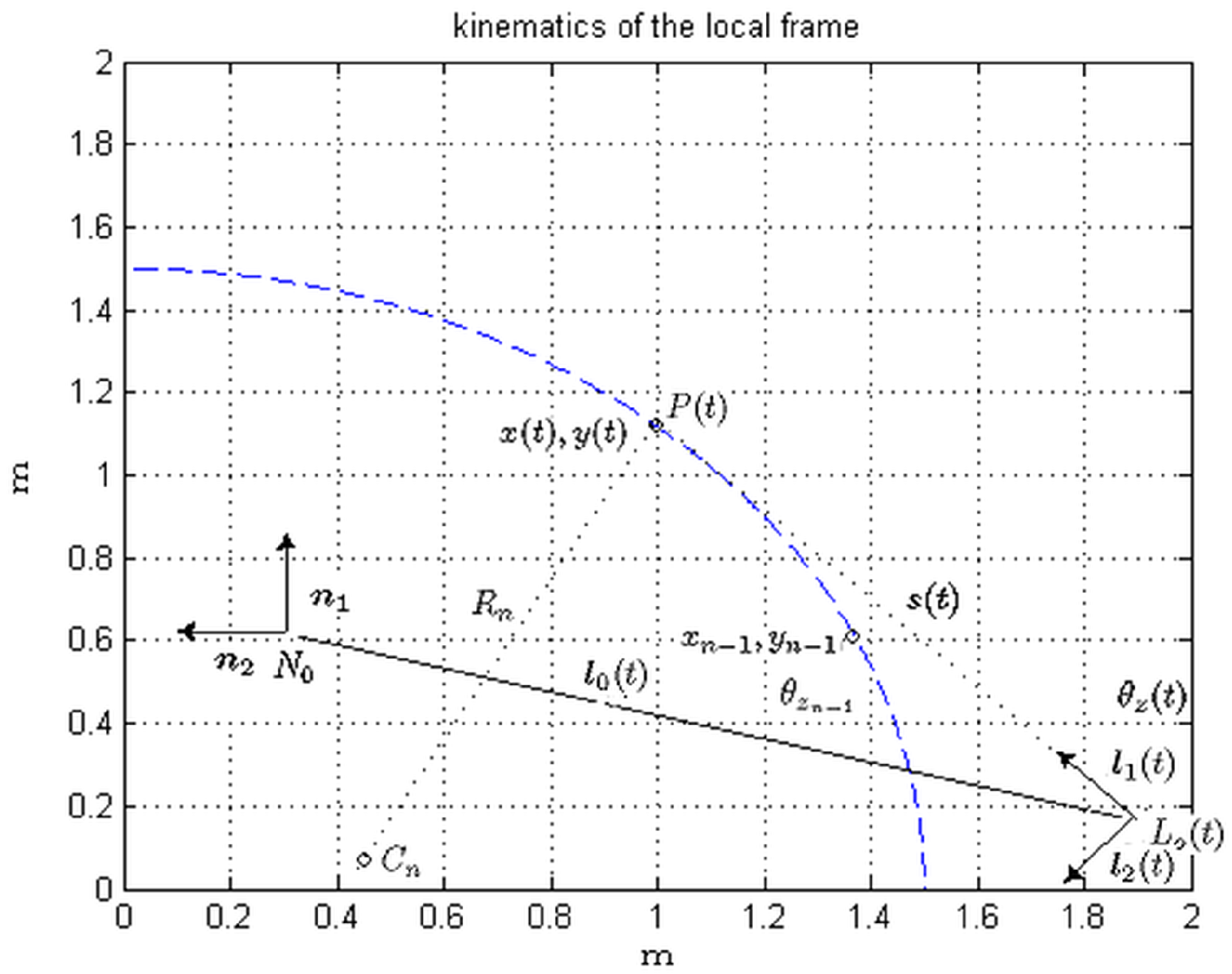
Indicate with N the inertial reference frame with origin $N_o$ and unit vectors ${\mathit{n}}_1,{\mathit{n}}_2,{\mathit{n}}_3$, according to the right-handed convention, ${\mathit{n}}_3$ being the vertical axis pointing upward. L is a local moving reference frame defined by its origin $L_o$ and unit vectors ${\mathit{l}}_1,{\mathit{l}}_2,{\mathit{l}}_3$. ${\mathit{l}}_1$ are aligned at each instant to the direction of walk tangent to the path curve, ${\mathit{l}}_2$ is orthogonal to ${\mathit{l}}_1$ on the horizontal plane and ${\mathit{l}}_3$ vertical, aligned with ${\mathit{n}}_3$. The plane ${\mathit{l}}_2-{\mathit{l}}_3$ is parallel to the frontal plane of the robot. The vector from $N_o$ to $L_o$ is indicated with ${\mathit{l}}_o$.

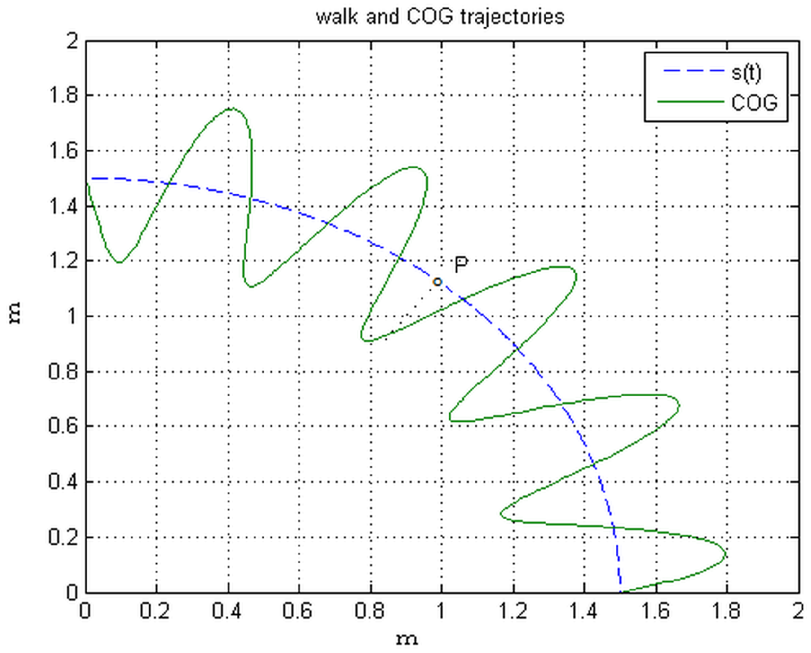
The point P is the current position at time t of the COG projection on the walk path, parametrized by its arc length $s\left(t\right)$. $\mathit{p}\left(t\right)$ is the vector from the $N_o$ to P, $x_L=s\left(t\right),y_L=0$ are the coordinates of P on the local frame, and $x\left(t\right),y\left(t\right)$, detailed later, on the inertial frame.

The walk path (see Figure 1) is a regular plane curve defined by its curvature (osculating circle) and its center of rotation (involute) as function of $s\left(t\right)$ [12]. In planning the trajectory the arc length will coincide with the preview of COG along x: $s=CO{G}_{x_{preview}}$. To generate an arbitrary path, radius and center of rotation change continuously. In practice, they are updated at every sampling time with radius $R_i,i=1,\cdots ,n$. The rotation around ${\mathit{n}}_3$ of the local frame L, coincident with that of the robot frontal plane, is defined during one sampling period by

$${\dot{\mathsf{\theta }}}_z\left(t\right)=\dot{s}\left(t\right)/R_i.$$

(2)

After $n-1$ sampling periods, at instant $t_{n-1}$, $s_{n-1},x_{n-1},y_{n-1}$ and ${\mathsf{\theta }}_{z_{n-1}}$ indicate, respectively, the arc length, the world coordinates $x,y$ and the orientation angle. The significant elements to define the kinematics of the local frame during the next $nth$ period, shown in Figure 2, are detailed as follows.

The rotation angle, from Equation (2) with radius $R_n$, is

$$\begin{array}{c}\hfill {\mathsf{\theta }}_z\left(t\right)={\mathsf{\theta }}_{z_{n-1}}+\underset{t_{n-1}}{\overset{t}{\int }}{\dot{\mathsf{\theta }}}_z\left(\mathsf{\tau }\right)·d\mathsf{\tau }.\end{array}$$

(3)

The center of rotation $C_n$ with respect to $N_o$ is defined by the vector

$${\mathit{c}}_{\mathit{n}}=(x_{n-1}-R_{n}sin\left({\mathsf{\theta }}_{z_{n-1}}\right)){\mathit{n}}_{\mathbf{1}}+(y_{n-1}+R_{n}cos\left({\mathsf{\theta }}_{z_{n-1}}\right)){\mathit{n}}_{\mathbf{2}},$$

(4)

using the last sampling position.

The current walk position $P\left(t\right)$ with respect ot $N_o$ is expressed using the center $C_n$ and the local reference frame L:

$$\mathit{p}\left(t\right)={\mathit{c}}_{\mathit{n}}-R_n{\mathit{l}}_{\mathbf{2}}\left(t\right).$$

(5)

Given $\mathit{p}\left(t\right)$, the origin of frame L, through the vector from $N_o$ to $L_o\left(t\right)$, is

$${\mathit{l}}_{\mathit{o}}\left(t\right)=\mathit{p}\left(t\right)-s\left(t\right){\mathit{l}}_{\mathbf{1}}\left(t\right),$$

(6)

i.e., $L_o\left(t\right)$ executes the involute of the path curve.

The current coordinates of $P\left(t\right)$ in N are obtained from the scalar products

$$x\left(t\right)=\mathit{p}\left(t\right)·{\mathit{n}}_{\mathbf{1}},y\left(t\right)=\mathit{p}\left(t\right)·{\mathit{n}}_{\mathbf{2}}.$$

(7)

In Appendix A , a fragment of the Autolev code used to generate the expressions for the real time computation of the necessary functions is presented.

4. Trunk and Feet Rotations

The trunk rotation simply follows continuously the angle ${\mathsf{\theta }}_z$ of rotation of the local reference frame as defined by Equation (3). This maintains the frontal plane orthogonal to the direction of walk during the whole stride period.

The feet, vice versa, follow a different rotation pattern, as they can rotate during the single stance period only, one at the time when they swing. Their velocity starts from and goes to zero during the acceleration and deceleration at $To{e}_{1}off$ and $Hee{l}_{2}strike$ (see part I for the definition of the gait), i.e., when they leave and touch the ground at each step.

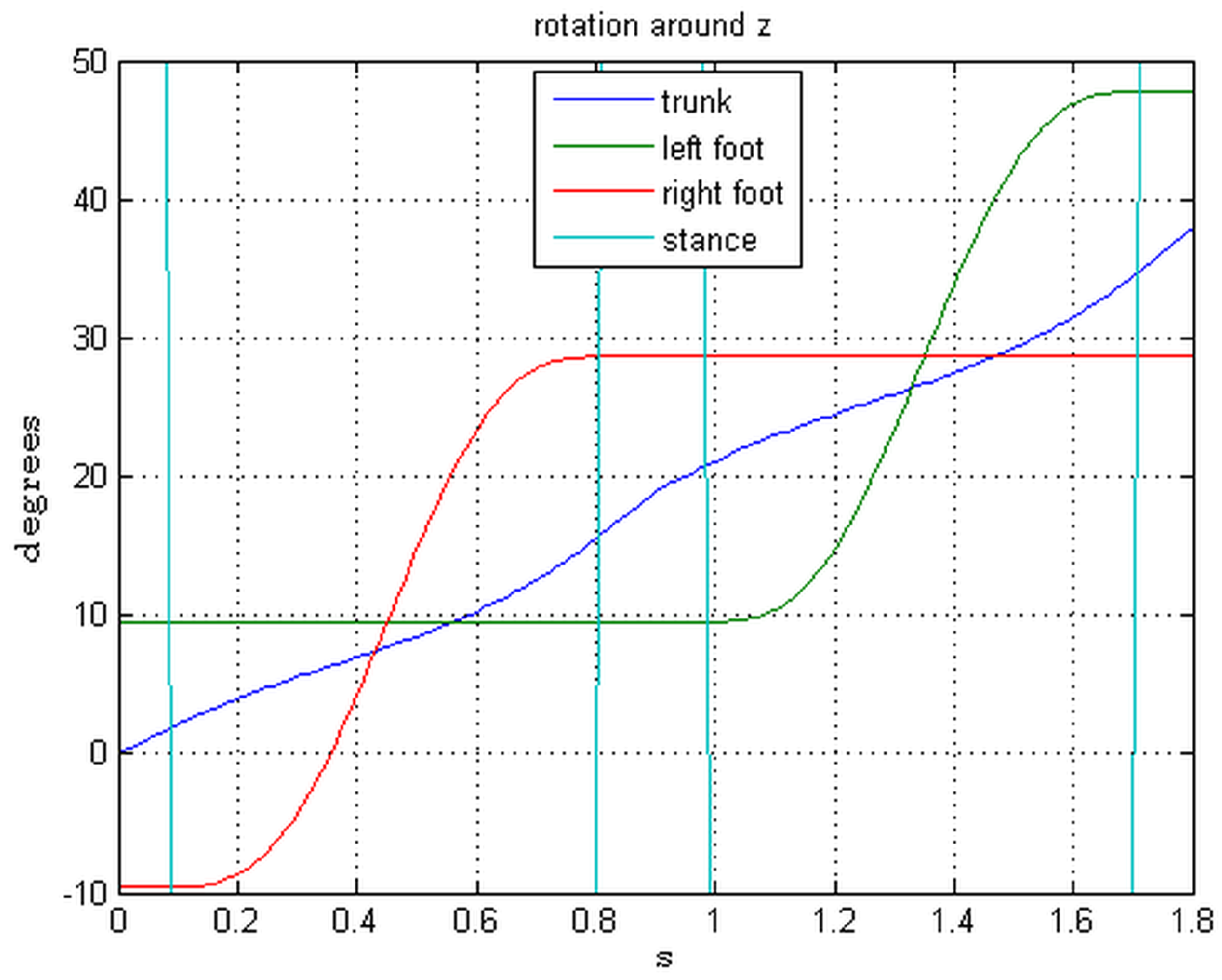
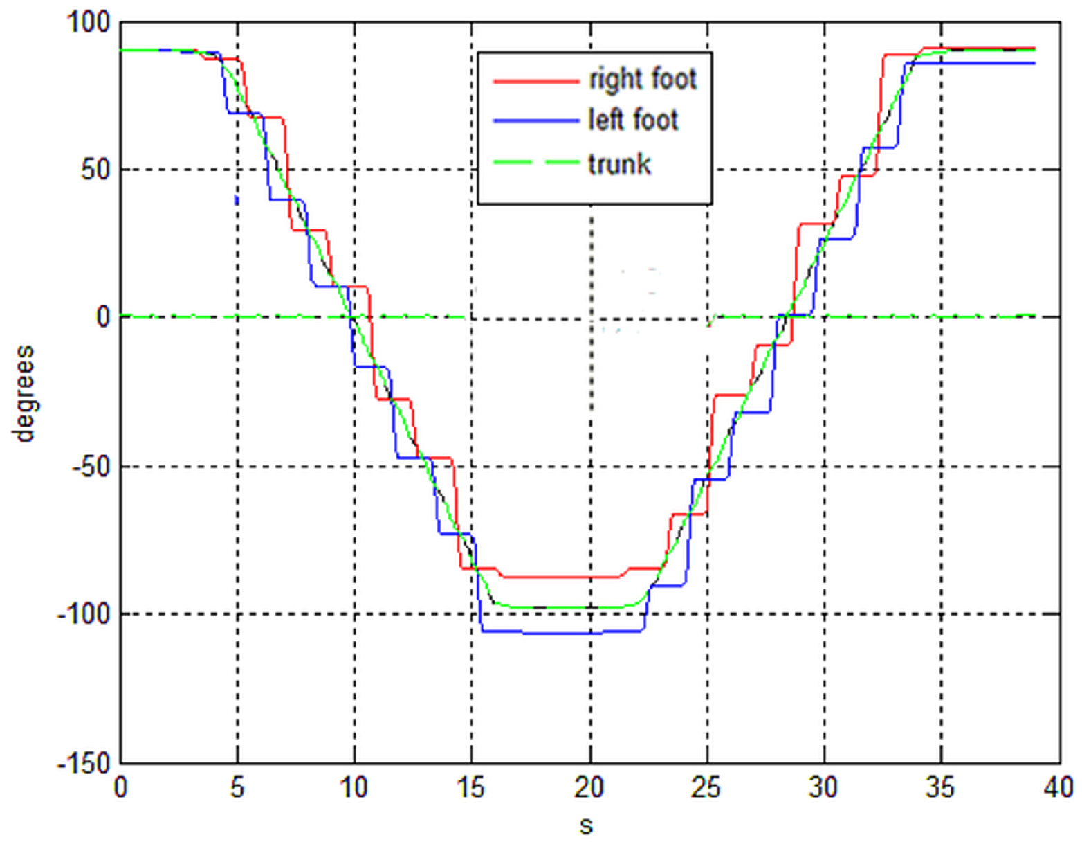
To maintain the pace of turn, a standard bell shaped pattern is adopted during the period of swing for the angle velocity of each foot, and its amplitude is controlled in real time by feedback, to ensure during a step that the mean of the angles of the two feet $({\mathsf{\theta }}_{foo{t}_1}+{\mathsf{\theta }}_{foo{t}_2}\left(t\right))/2\cong {\mathsf{\theta }}_{trunk}\left(t\right)={\mathsf{\theta }}_z\left(t\right)$ follows the trunk angle. The result is shown in Figure 3. The small misalignment between trunk and feet angles is due to the feedback sampled at each step period.

5. COG and Feet Reference Trajectories in Local Frame

In the local reference frame that accompanies the turn of the robot, $CO{G}_{x_{preview}}$ and $CO{G}_{y_{preview}}$ along ${\mathit{l}}_{\mathbf{1}}$ and ${\mathit{l}}_{\mathbf{2}}$ remain almost unchanged with respect to the rectilinear walk. Only $CO{G}_{y_{preview}}$ has to be corrected by an offset so as to compensate for the centrifugal acceleration influencing $ZM{P}_y$. In fact, during the turn, the $ZM{P}_y$ is not only affected by the accelerations and decelerations of the $CO{G}_y$ but also by the centrifugal acceleration due to the speed of rotation. Adopting the standard linearized inverted pendulum approximation, the actual $ZM{P}_y$ is given by

$$ZM{P}_y=CO{G}_y-CO{G}_z/g·({\ddot{COG}}_y+{{\dot{COG}}^2}_x·(R_n-CO{G}_y)/{R_n}^2)$$

(8)

Thus, in order to guarantee the desired position of the $ZMP$ on L, the following a priori correction term must be added to the original $CO{G}_{y_{preview}}$ for rectilinear walk:

$$CO{G}_z/g·{{\dot{COG}}^2}_x·(R_n-CO{G}_{y_{preview}})/{R_n}^2$$

(9)

Moreover, using the extended $COG/ZMP$ estimator outlined in the Appendix A of Part II, this acceleration is detected as an external disturbance and a further a posteriori correction is introduced.

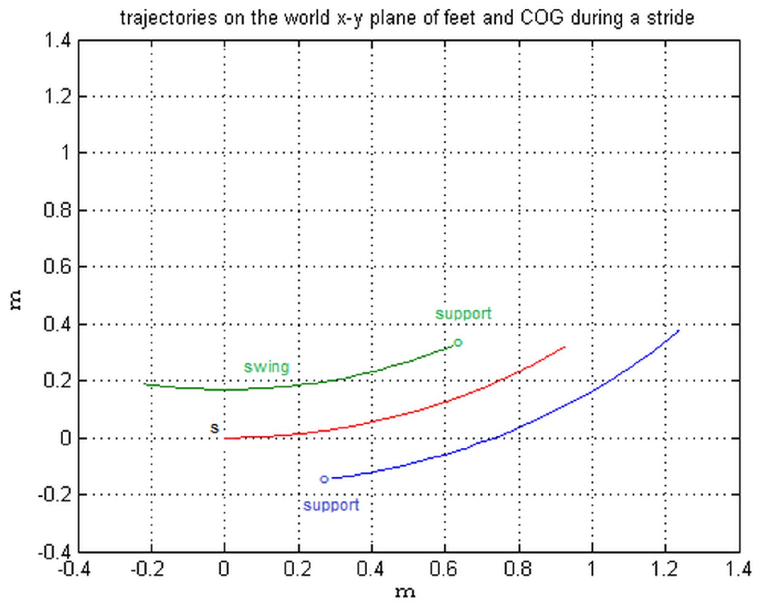
The reference trajectories (along x and y) of the swing foot, also, require a modification, to take into account the relative motion of the local frame with respect to the world frame. To easily understand and as an example, one stride following an ideal circular path is performed in Figure 4, and in Figure 5 and Figure 6, the trajectories along $x_L$ and $y_L$ are compared with those of the rectilinear walk, i.e., $R=\infty$, drawn in dashed lines.

Circularity during a step in reality is not a stringent requirement, as these trajectories are generated in real time to adapt to the actual path, as described in the next subsections.

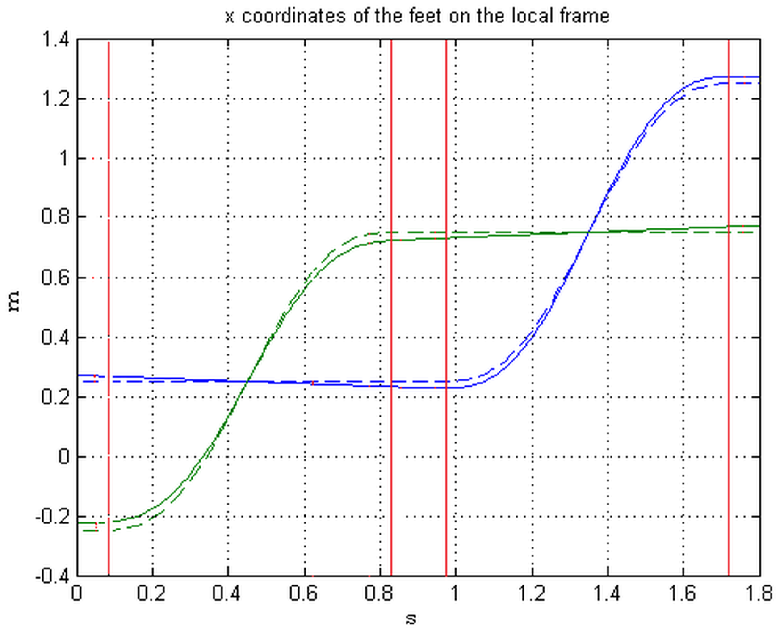
5.1. Implementation of the Swing Foot Reference along ${\mathit{x}}_{\mathit{L}}$

In the rectilinear walk, the velocity of the swing foot along x is similar to a bell shaped function with an integral equal to twice the step length $ste{p}_L$ on a time interval equal to the single stance period. In fact, in the rectilinear walk, a symmetrical or skewed standard bell function is taken as reference of the velocity, and its amplitude is adaptively corrected in real time to maintain the feet aligned with the $ZM{P}_x$.

In the walk with turns, this will not be sufficient, and a correction must be added to the original trajectory to be computed step by step in order to zero the forward velocity of the foot on the world reference at contact with the ground.

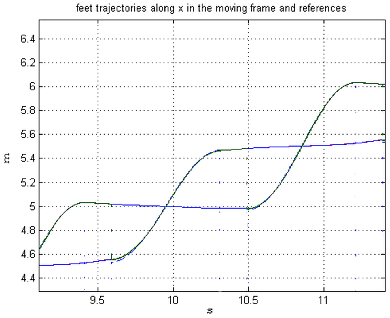
Figure 4 shows the center path of the COG and the trajectories of the two feet during a stride; the forward foot (blue line) will initially support the step. In Figure 5, the x coordinates of the feet on the moving frame L are plotted, the difference with respect to the rectilinear walk, drawn with dashed lines, is evident, and analyzed more closely.

The position and velocity of the center of the supporting foot during the period of time it remains on the ground, i.e., a step plus a double stance period, is computed with the technique of generating the involute of an arc of a circle described in Section 3. Indicating the arch length with s, and considering that at the end of the double stance the foot that will support the next swing advances the COG position of one step length, the following equations result:

$$\begin{array}{cc}\hfill x_{Foot{1}_L}\left(s\right)& =s+(R+L_{feet}/2·phase)·sin((0.5·ste{p}_L·(ste{p}_P+d{s}_P)/ste{p}_P-s)/R)\hfill \\ \hfill {\dot{x}}_{Foot{1}_L}\left(s\right)& =(1-(1+L_{feet}/2·phase)·cos((0.5·ste{p}_L·(ste{p}_P+d{s}_P)/ste{p}_P-s)/R)·ste{p}_L/ste{p}_P\hfill \\ \hfill 0& \le s\le ste{p}_L·(ste{p}_P+d{s}_P)/ste{p}_P.\hfill \end{array}$$

(10)

On the rectilinear walk, those equations are simply:

$$\begin{array}{cc}\hfill x_{Foot{1}_L}& =ste{p}_L/2·(ste{p}_P+d{s}_P)/ste{p}_P\hfill \\ \hfill {\dot{x}}_{Foot{1}_L}& =0\hfill \end{array}.$$

(11)

$L_{feet}$ is the distance between the two feet along the y axis, $phase=\pm 1$ according to whether the center of rotation is at the right or left of the supporting foot, $ste{p}_L$ and $ste{p}_P$ are the step length and period, $d{s}_P$ is the period of double stance.

With $x_0,x_1,{\dot{x}}_0,{\dot{x}}_1$ the position and velocity of the correction term for the swing foot at the beginning and end of a single stance period is indicated. Note that the beginning of the swing period corresponds in Equation (10) to $s=ste{p}_L·(ste{p}_P+d{s}_P)/ste{p}_P$ and the end to $s=0$. From the difference between Equations (10) and (11), it results that positions and velocities of the correction term at the beginning and end of the swing interval are:

$$\begin{array}{cc}\hfill x_0=& -x_1=(R+L_{feet}/2·phase)·sin((0.5·ste{p}_L·(ste{p}_P+d{s}_P)/ste{p}_P-s)/R)\hfill \\ \hfill {\dot{x}}_0=& {\dot{x}}_1=(1-(1+L_{feet}/2·phase)·cos(0.5·ste{p}_L·(ste{p}_P+d{s}_P)/ste{p}_P/R)·ste{p}_L/ste{p}_P\hfill \end{array},$$

(12)

i.e., at the extremes, positions have opposite values and velocities are identical.

Measuring $x_0$ and ${\dot{x}}_0$, and assuming as initial position $x_0$, initial velocity ${\dot{x}}_0$ and final position $-x_0+{\mathsf{\delta }}_x$, a third order polynomial for the correction during the next single stance period is derived at each step. ${\mathsf{\delta }}_x$ has been introduced to adapt, by feedback in real time at each step, the correction to the real path.

To obtain the new reference trajectory, this correction is added to the original one of the rectiliear walk.

5.2. Implementation of the Swing Foot Reference along ${\mathit{y}}_{\mathit{L}}$

Without turns, the feet motion along y is zero, as it does not deviate from a baseline at a constant distance from the walk path. Vice versa, when the moving frame rotates, a correction has to be considered.

In the ideal condition of Figure 4, the trajectory of the swing foot on L to connect two successive support periods is shown in Figure 6. It starts and ends approximately at the same value, with the opposite derivative, reaching near the mid-distance the baseline of the rectilinear walk. To interpolate this function, a fourth order polynomial is necessary.

Let $y_0$ and $\dot{y_0}$ be the position and velocity of the foot center along ${\mathit{l}}_2$ at the end of the previous double stance period. Choose $y_1=y_0+{\mathsf{\delta }}_Y$, $\dot{y_1}=-\dot{y_0}$ as values of the position and its velocity at the end of the next single stance period, and $y_m=L_{feet}/2·phase$ the position at mid-distance. With these five values, a fourth order polynomial is computed in real time for the reference trajectory to be used for the next single stance period. As in the previous section, ${\mathsf{\delta }}_y$ is used in feedback, step by step, to adaptively bring the feet trajectory at the end of the single stance to $ZM{P}_y$.

6. A Simulation Example

The following figures show the results of the dynamical simulation of the control of a model identical to the one in the previous part II, i.e., a man 1.78 m tall of 75 kg wearing an exoskeleton of 30 kg during an “S” shaped path, with a distance between the feet of 0.34 m, a step length of 0.5 m, a step period of 0.9 s, and a double stance interval of 0.18 s. The control and the example are identical to those of part II, and the description of the simulator built at Politecnico di Torino is contained in part I. There, in particular, the critical issues related to the contact between feet and ground are discussed.

The path was obtained as described in Section 3 with a sampling period of 10 ms, a radius changing at a rate of 7.5 during the time of a step, with a minimum value of 2 m.

In Figure 7, the rotational angles of trunk and feet are shown. The non-perfect symmetry of the feet angles is a consequence of the feedback with sampling interval of the step period. However, it is argued that this will be of no consequence.

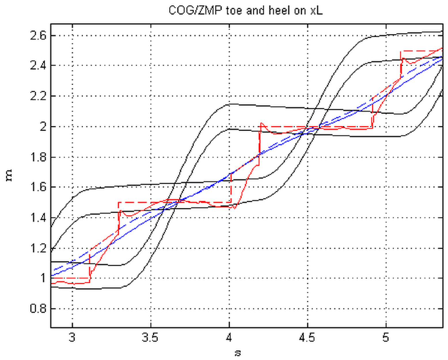
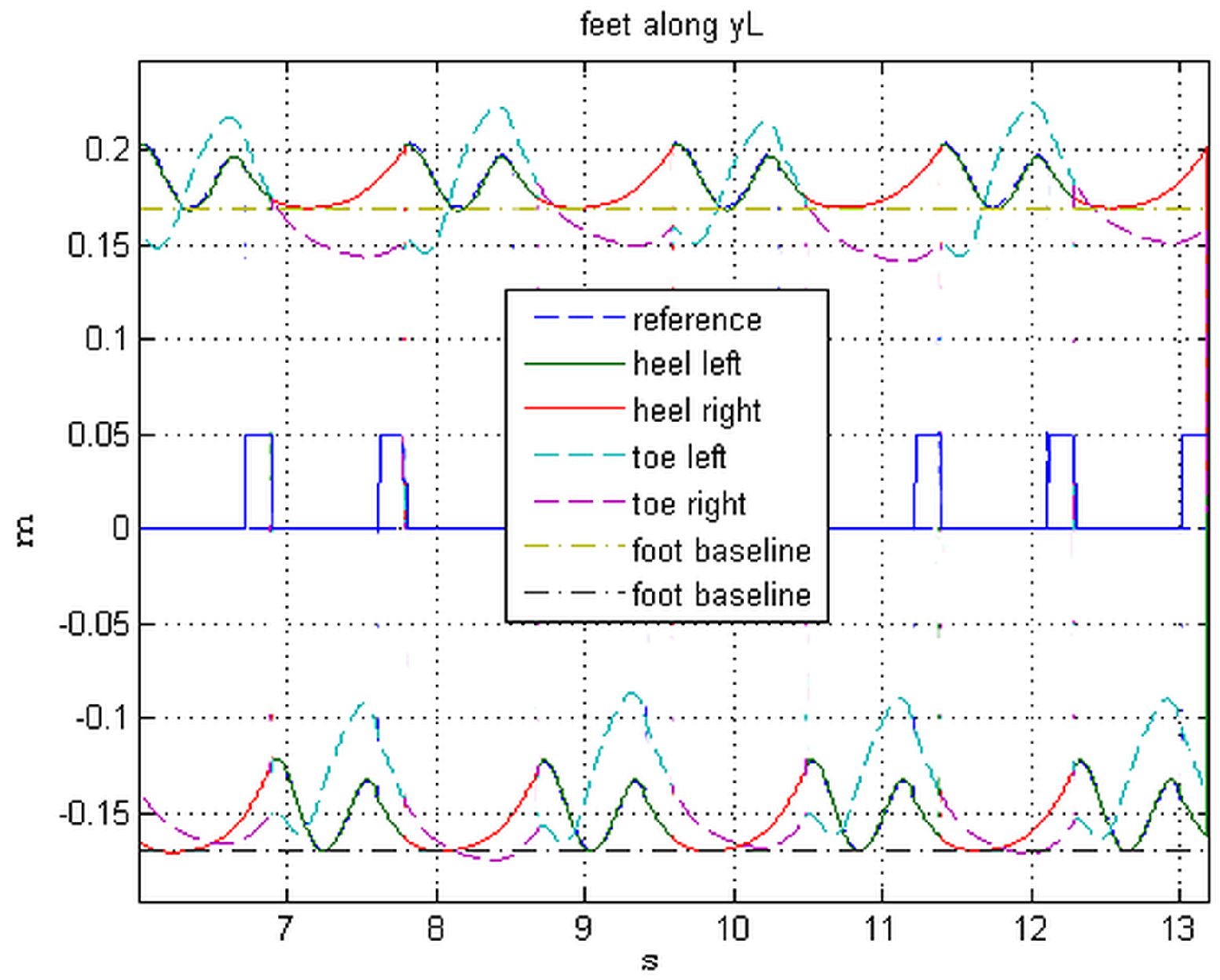
The $y_L$ coordinates of the feet are shown in Figure 8. During the swing period, the reference and its tracking can be seen. The effect of the feedback in maintaining the feet on the baseline is evident.

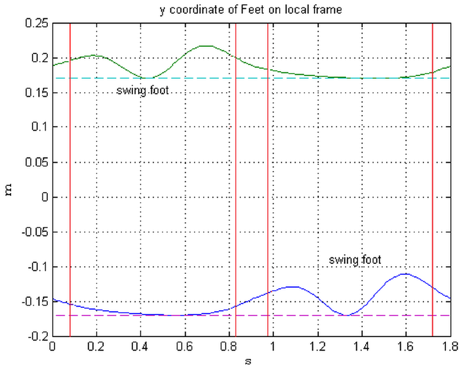
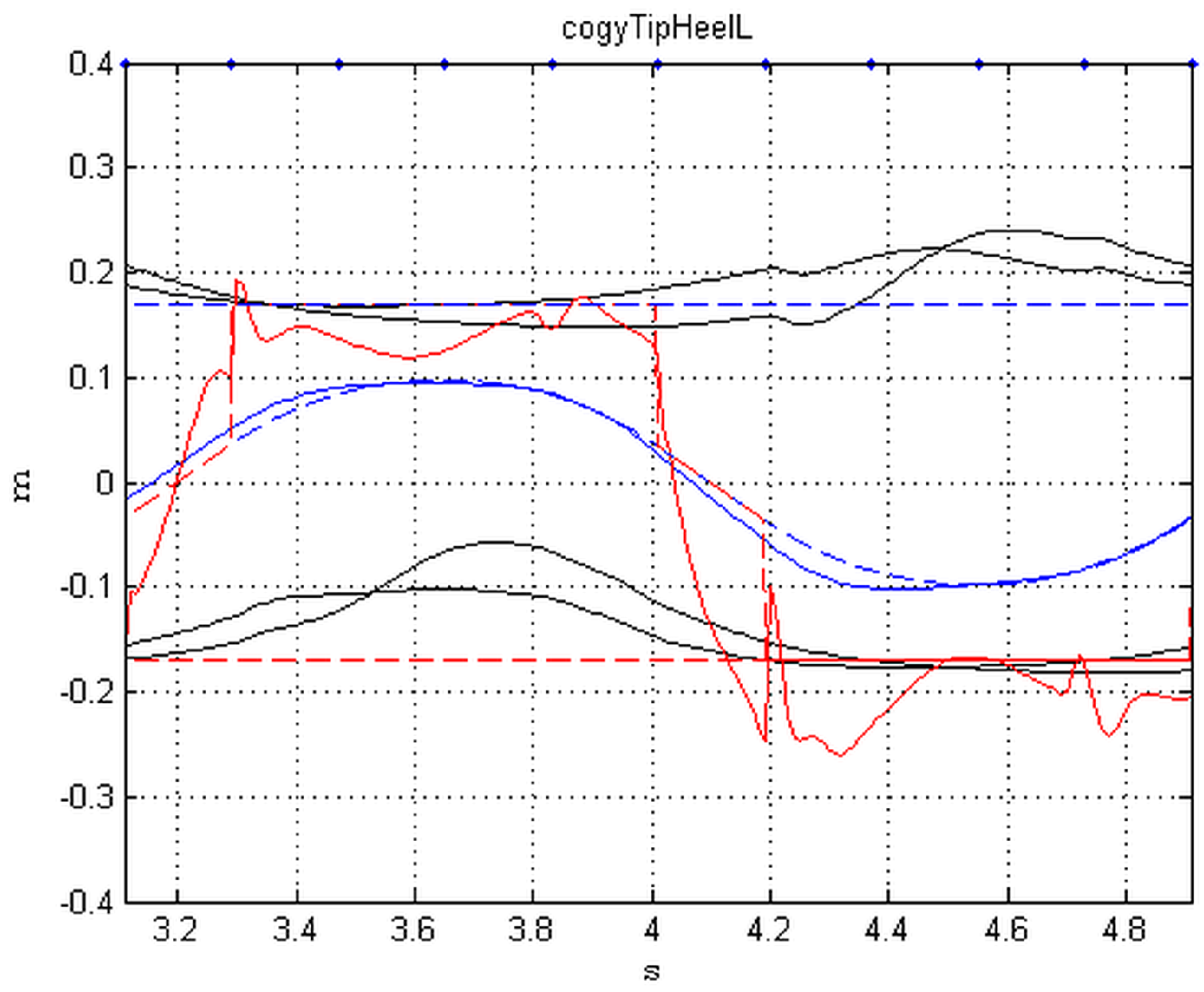
Similarly, Figure 9 shows the tracking of the swing feet $x_L$ coordinates. The reference during single stance is shown as a dashed line.

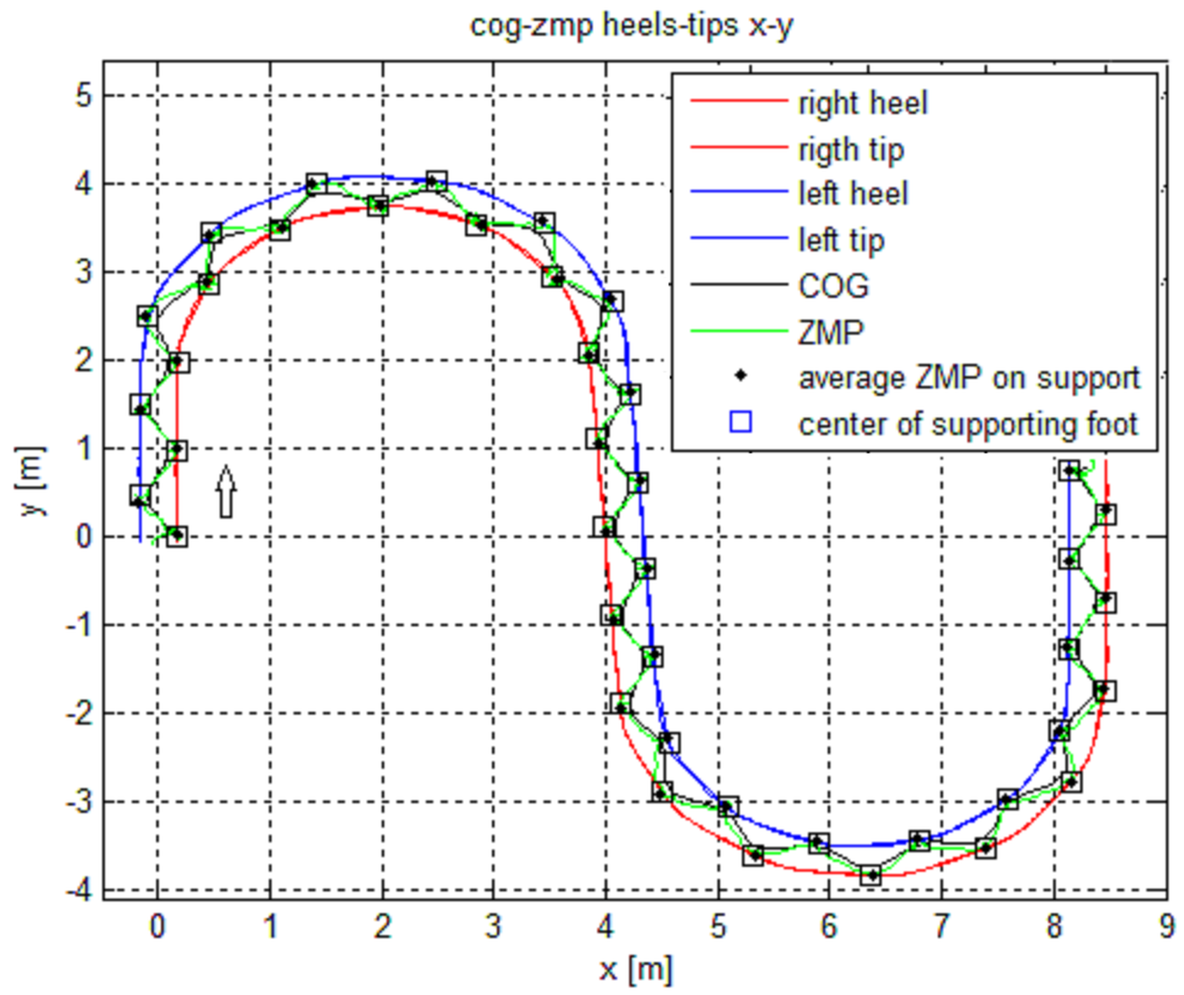
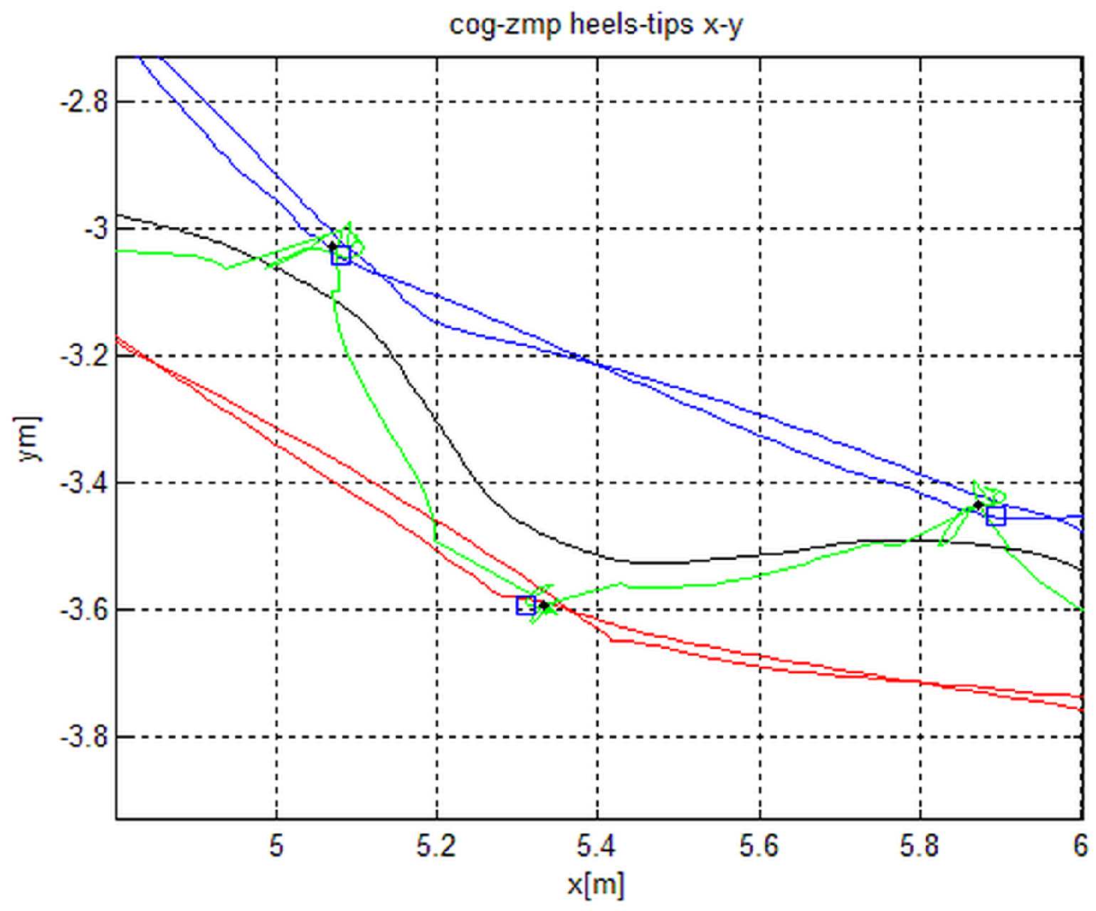
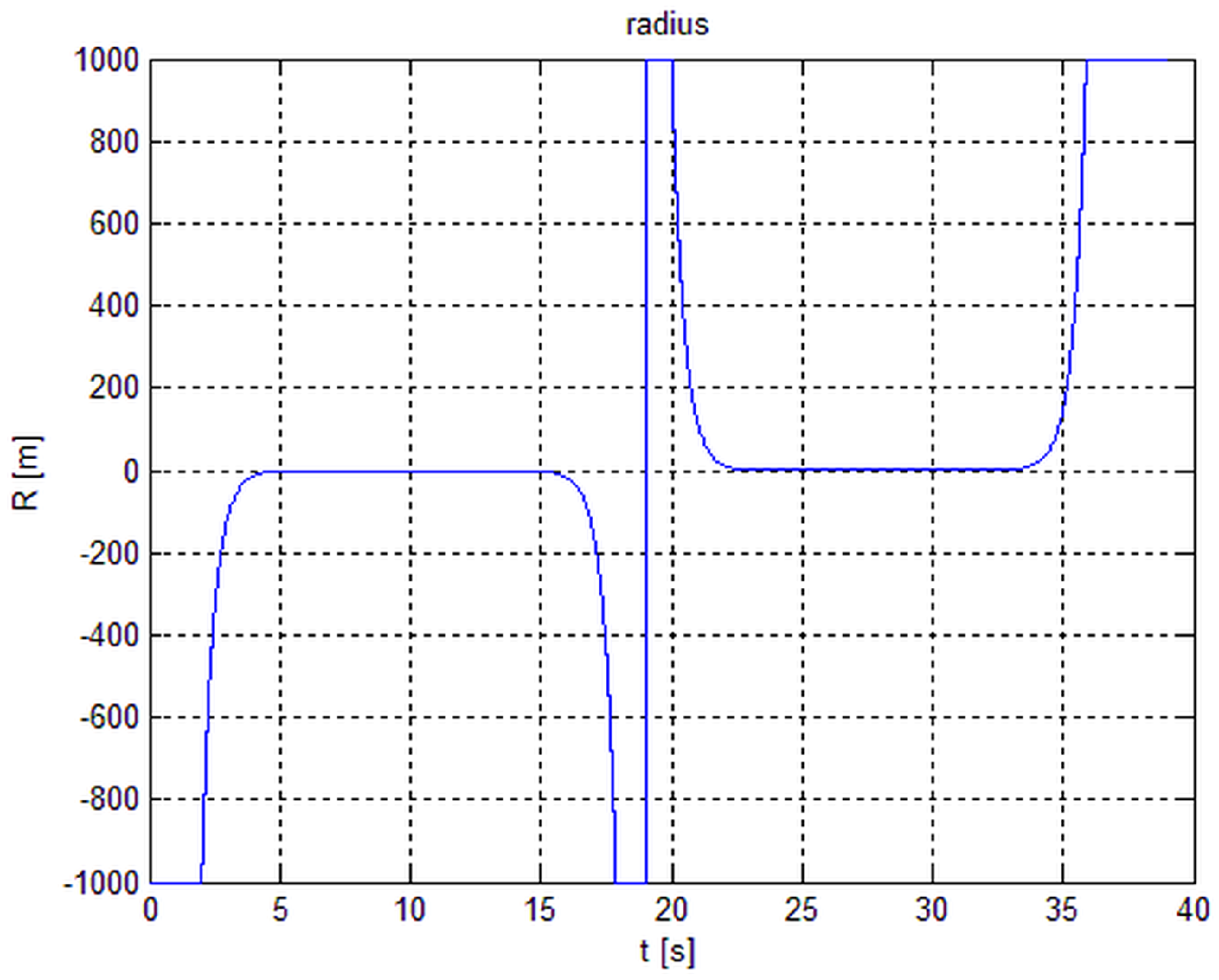
The trajectories of toes, heels, COG and ZMP on the horizontal plane of the world frame are presented in Figure 10, with details in Figure 11. Note the position of the center of the supporting foot and the average of the point cluster of the ZMP on the support. The behavior of the radius that generates the path is in Figure 12.

Figure 13 and Figure 14 show the behavior of COG, ZMP, tips and heels in the local frame during one stride.

The blue line is the COG behavior (the dashed line is the reference), the red line is the ZMP, the black lines are heel and toe. The rectilinear dashed lines in Figure 14 indicate the baselines of the two feet.

7. Conclusions

An extension of the rectilinear walk of a biped to the walk with turns has been presented. It is obtained by transferring a rectilinear walk and the tracking of reference trajectories on a Cartesian moving frame that accompanies the turns of the curvilinear path in addition to controlling the joints using the appropriate Jacobian matrix from joint space to this moving space. The path curve of the walk can be arbitrary and is generated in real time by changing the radius of curvature at each sampling time.

A minimalistic approach has been adopted in the definition of the reference trajectories, with the aim to generate and adapt them in real time. This accounts for bell shaped functions, third and forth order polynomials, whose parameters are corrected by feedback in order to maintain a coherent walking pattern.

The inconsistency of these (somewhat arbitrary) trajectories with the multichain kinematics of the biped was accomodated, as shown by the simulations, by the adoption of the “extended Jacobian” and weighted least squares of part II. With the objective of adaptively providing a reference pattern for the biped, a further extension toward a completely free walk, is the on line change of the gait parameters $L_{feet}$, $ste{p}_P$, $ste{p}_L$, $d{s}_P$. This is actually under investigation and will be the object of future works.