High-Precision Static Calibration of Capacitive Sensing in Inertial Sensors via Image-Based Displacement Measurement and Bias Modeling

Abstract

Space gravitational wave detection missions demand ultra-stable calibration of inertial sensor capacitive sensing. Conventional dynamic methods suffer from mechanical vibration noise and bias separation difficulties, while large-displacement operation introduces pronounced nonlinearity. This work proposes a static calibration method using an image-based displacement measurement system to establish a vibration-free benchmark. A subpixel edge detection algorithm locates the Test Mass and Electrode Housing edges with a repeatability of approximately 0.05 pixels, and the Test Mass geometry is independently calibrated by a Coordinate Measuring Machine (CMM, ±2 µm, $k=2$) to provide SI traceability. A nonlinear calibration model incorporating higher-order Taylor terms is developed, combined with a forward/reverse connection technique for composite bias modeling. Experimental validation at $x_0=665$ µm ($x_0/d_0\approx 0.665$) demonstrated a gain coefficient repeatability of 0.01658% RMSPER and a combined expanded uncertainty of $U\approx 2.18\times {10}^{-5}$ $1/\mathsf{\mu }\mathrm{m}$ ($k=2$). Intended as a complementary ground-based technique to dynamic calibration, this method avoids dynamic excitation-induced noise while establishing complete SI traceability, offering a reliable solution for ground validation and long-term monitoring of space inertial sensors.

1. Introduction

In ultra-precision measurement tasks such as space gravitational wave detection (e.g., LISA, Taiji, TianQin program) [1,2,3,4], Global Gravity Field Measurement [5,6,7], and Verification of the Equivalence Principle [8,9], the accuracy of capacitive displacement measurement in inertial sensors directly determines the success of scientific objectives, imposing stringent requirements for stability and accuracy in their calibration techniques. Ground-based validation of these space-borne sensors frequently relies on torsion pendulum facilities and high-precision optical readout systems to simulate the in-orbit environment and characterize sensor performance prior to launch [10,11,12]. For the TianQin mission, a high-precision capacitive displacement transducer with a noise requirement of $6.9\times {10}^{-7}\mathrm{pF}{\mathrm{Hz}}^{-1/2}$ at 6mHz has been developed [13]. As a core payload, the inertial sensor primarily consists of a high-precision sensitive structure and its front-end electronics unit [14]. High-precision capacitive sensing architectures for space inertial reference sensors have been extensively developed to meet the stringent noise and stability requirements of gravitational wave detection missions [15]. The capacitive sensing module is responsible for precisely detecting the relative displacement between the Test Mass (TM) and its surrounding Electrode Housing (EH), providing critical feedback for the closed-loop control system. However, due to tolerances in electronic components and machining errors, the actual gain of the capacitive sensing circuit often deviates from the design value. Therefore, before the spacecraft enters orbit, a highly reliable ground calibration system must be established to accurately calibrate its gain and bias parameters. Beyond displacement sensing for drag-free control, capacitive transducers are also fundamental for other critical operations, such as the measurement and management of the test mass charge, which is essential to mitigate electrostatic forces that could compromise sensor performance [16].

Traditional dynamic calibration methods (e.g., based on piezoelectric platforms or precision displacement stages) are widely employed for in-orbit and ground-based characterization, yet they introduce difficult-to-quantify mechanical vibrations and dynamic errors during excitation, which complicate the precise separation of bias components and limit the repeatability of calibration results [17]. Although capacitive sensors are highly regarded for their sensitivity, existing research predominantly focuses on dynamic response characteristics [17], leaving significant theoretical gaps in nonlinear error compensation and bias voltage modeling for static calibration. For instance, Fichter et al. [18] used Kalman filtering for capacitive circuit calibration but did not employ the actual sensitive structure, failing to reflect coupling errors under real operating conditions. Although previous studies have utilized a real sensitive structure and proposed a linear model for bias voltage, the piezoelectric sinusoidal motion excitation method they relied upon still suffers from inherent instability issues. Further research by Gan et al. [19] indicated that circuit asymmetry introduces a DC bias proportional to the detection voltage, yet effectively separating this dynamically coupled component from a fixed offset remains a challenge for existing techniques. It should be emphasized that dynamic methods remain indispensable for in-orbit calibration and multi-degree-of-freedom characterization; the static approach proposed herein is intended to complement, rather than replace, these techniques by providing a ground-based benchmark free from vibration-induced artifacts.

Notably, regarding static calibration methodology, Li et al. [20] used an eight-point conductive rubber structure and the least squares method to achieve static calibration of a six-dimensional force sensor, but the coupling error remained as high as 15.24%, and no circuit bias modeling was performed. On the other hand, the study by Yang et al. [21], which fused quasi-static and dynamic calibration to suppress dynamic errors, highlighted the critical role of static benchmarks in improving calibration accuracy, providing important methodological inspiration for the purely static approach adopted in this paper. These studies reveal both the value of static benchmarks and the shortcomings of existing static schemes in improving accuracy and compensating for circuit errors.

In the field of high-precision dimensional metrology, image-based measurement techniques have been widely adopted as non-contact solutions for traceable displacement quantification. Recent advances in subpixel edge detection algorithms have enabled vision systems to achieve accuracies approaching the nanometer level. For instance, Yuan et al. [22] proposed a telecentric imaging calibration method integrating subpixel edge detection with illumination error compensation, achieving reprojection errors of 0.059 pixels and measurement deviations within 1.6 µm for CMM-verified artifacts. Lou et al. [23] developed a binocular camera calibration method based on partial-area-effect subpixel edge detection, improving calibration accuracy by 23% under conventional environments. Furthermore, Moru and Borro [24] demonstrated a machine vision inspection system operating at the subpixel level, validated against CMM ground-truth measurements with a calibration error of 0.06 pixels. These developments build upon foundational work in subpixel edge detection, including the polynomial fitting approach by Steger [25] and the moment-based method by Tabatabai and Mitchell [26], which established the theoretical framework for subsequent Gaussian-integral and illumination-compensated techniques. These studies indicate that the combination of CMM-traceable geometric references, high-resolution industrial cameras, bi-telecentric lenses, and subpixel edge detection constitutes a reliable metrological chain for static displacement benchmarking. In this work, the 46 mm side length of the TM, independently calibrated by a CMM with an expanded uncertainty of ±2 µm ($k=2$), serves as the SI-traceable reference for pixel-equivalent determination, while a Touptek IUA25000KPA industrial camera (25 MP, 5120 × 5120) equipped with a Myutron FTV03C-110 bi-telecentric lens (0.28× magnification) and a subpixel edge detection algorithm are employed to locate the TM–EH edges with an accuracy of approximately 0.05 pixels.

A fundamental challenge in static calibration is establishing a traceable, non-contact displacement reference. Conventional contact-based displacement gauges, such as dial indicators or LVDTs, introduce mechanical reaction forces that may disturb the TM–EH interface, and their resolution can become a limiting factor in sub-micron-level uncertainty budgets. Image-based measurement offers a non-contact, high-resolution alternative: the camera sensor functions as a dense two-dimensional displacement transducer, and the pixel equivalent is directly anchored to the CMM-calibrated TM geometry, establishing a complete SI-traceability chain from the CMM-calibrated length standard to the pixel level. In this context, the proposed image-based static calibration is intended to serve as a complementary ground-based technique to existing dynamic methods, providing a vibration-free displacement benchmark particularly suited for scenarios demanding absolute mechanical stability and direct geometric traceability.

It is emphasized that the proposed static method is positioned as a complementary ground-based technique to existing dynamic calibration approaches (e.g., piezoelectric platform excitation), not as their replacement. A direct experimental comparison would require simultaneous deployment of a dynamic excitation stage and the image-based static fixture within the same apparatus, which is beyond the scope of the present proof-of-concept study. Qualitatively, the static method eliminates actuator-induced vibration noise, hysteresis, and thermal drift—error sources that are inherent in dynamic methods and reported in the literature (e.g., RMSPER ∼0.02% for piezoelectric platforms under temperature control). The achieved static RMSPER of 0.01658% demonstrates competitive stability, albeit in a simpler single-DoF configuration. Future work will include a side-by-side metrological comparison once the dynamic stage is integrated.

To address the aforementioned challenges, this paper proposes a static calibration method for inertial sensor capacitive sensing based on image-based displacement measurement and bias modeling. This method establishes a stable displacement benchmark by fixing the TM at an extreme static position within the EH and rigidly locking the alignment mechanism; the resulting gap distance is precisely quantified using a high-resolution image-based measurement system. The method thereby establishes a complete metrological traceability chain: the Test Mass geometry (46 mm side length) is first independently calibrated using a Coordinate Measuring Machine (CMM, ±2 µm expanded uncertainty, $k=2$), providing an SI-traceable length standard for subsequent pixel-equivalent calibration via subpixel edge detection. As a complementary ground-based technique, this approach avoids dynamic excitation-induced noise while offering direct geometric traceability, particularly suited for laboratory validation where absolute mechanical stability is required. Simultaneously, combined with the forward/reverse connection testing technique, a composite bias model including a detection voltage-dependent term (${\delta }_0{U}_d$) and a fixed offset term ($u_c$) is established. Experimental results demonstrate that the calibration repeatability for the gain coefficient (measured by RMSPER) reaches 0.01658%.

A key contribution of this work is the extension of the static calibration method’s applicability to effectively handle large-displacement scenarios. The operational modes of space inertial sensors include the science mode (±10 µm) and the capture mode (±200 µm). In the capture mode, the ratio of displacement x to the capacitive gap $d_0$ (typically 1 mm) increases significantly, making the nonlinearity of the capacitance change pronounced. Consequently, the traditional linear model (retaining only the first-order term in the Taylor expansion) becomes inadequate. By systematically incorporating higher-order terms such as $x^3/d_0^2$ and $x^5/d_0^4$ into the calibration model, this paper establishes a more accurate nonlinear calibration model, supporting high-precision displacement measurement for inertial sensors in large-displacement scenarios like the capture mode.

Experimental verification shows that this method not only exhibits excellent repeatability (RMSPER <0.02%) but also, through systematic uncertainty analysis, clarifies its path for accuracy improvement. This research aims to provide a simple-to-operate and reliable technical solution for the on-orbit calibration and long-term performance monitoring of space inertial sensors. Furthermore, the static calibration approach based on CMM-traceable image-based benchmarks employed in this method also offers a possible reference for other high-precision static/quasi-static displacement measurement systems sensitive to vibration.

2. Capacitive Sensing Calibration Model

2.1. Theoretical Model of the Sensing Circuit

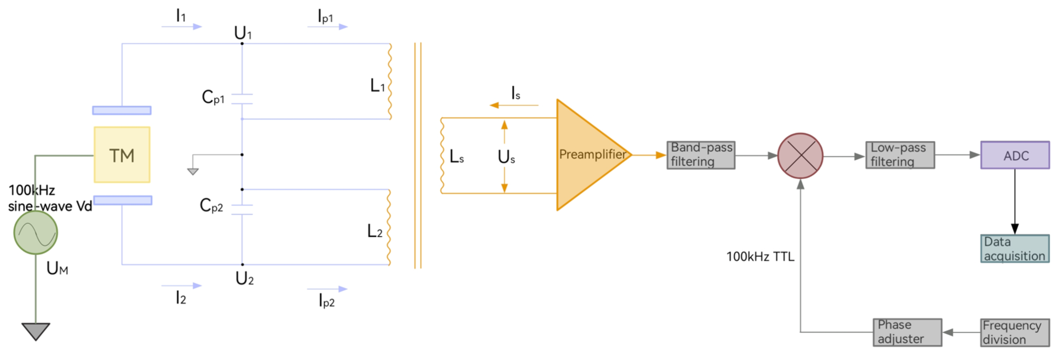
The precision measurement process of the capacitive displacement sensor follows a multi-stage physical signal conversion chain. As illustrated in Figure 1, the modular circuit architecture comprises six principal stages:

• Displacement-to-capacitance conversion: Symmetric electrode pairs (Electrode Tiles, ETs) etched on the TM and EH surfaces form a differential capacitance structure, achieving linear conversion from sub-micron displacement to femto-farad-level differential capacitance.
• Differential Capacitance Amplifier (DCA): Performs primary amplification of the weak capacitance change through a high-precision current-to-voltage conversion circuit.
• Bandpass Filter (BPF): Implements narrowband selective amplification at the carrier frequency, effectively suppressing inherent $1/f$ noise and high-frequency interference.
• Phase-sensitive demodulation: Composed of a multiplier and a low-pass filter, this unit demodulates the required small-magnitude slow-varying signal from the amplitude-modulated carrier. By translating the baseband signal to an AC carrier, the influence of $1/f$ noise and amplifier DC drift is effectively prevented.
• Carrier and reference: A 100 kHz sinusoidal detection voltage $V_d$ is applied to the TM via the transformer bridge. An independent 100 kHz TTL square wave serves as the demodulation reference to synchronize the phase-sensitive demodulator.
• Analog-to-Digital Converter (ADC): Completes signal digitization, providing high-resolution data for the subsequent closed-loop control system.

This multi-stage architecture, through the synergistic optimization of frequency-division multiplexing and synchronous demodulation, ensures nanometer-level displacement detection accuracy while enhancing electromagnetic compatibility and noise suppression.

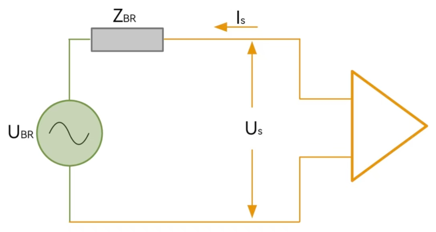
The preamplifier treats the sensing bridge as an equivalent voltage source ${\tilde{U}}_{BR}\left(\omega \right)$ in series with the bridge source impedance $Z_{BR}\left(\omega \right)$, as shown in Figure 2.

2.2. Displacement Detection Principle

The sensing structure operates on the parallel-plate capacitor principle, detecting the differential capacitance change caused by micro-displacement between the ET and the TM. As shown in Figure 3b, when the distance between the ET plane and the TM plane is $d_0$, the static capacitance is

$$C={\displaystyle \frac{{\epsilon }_0{\epsilon }_{r}A}{d_0}},$$

(1)

where ${\epsilon }_0=8.854\times {10}^{-12}\mathrm{F}/\mathrm{m}$ is the vacuum permittivity, ${\epsilon }_r=1$ is the relative permittivity (in vacuum), and A is the effective opposing electrode area.

When the TM undergoes a displacement x along the sensing axis (Figure 3c), the distances to the two electrodes change asymmetrically, yielding a differential capacitance

$$2\mathsf{\Delta }C={\displaystyle \frac{{\epsilon }_0{\epsilon }_{r}A}{d_0-x}}-{\displaystyle \frac{{\epsilon }_0{\epsilon }_{r}A}{d_0+x}}={\displaystyle \frac{2{\epsilon }_0{\epsilon }_{r}Ax}{d_0^2-x^2}}.$$

(2)

Performing a Taylor expansion of Equation (2) about $x=0$ gives

$$\mathsf{\Delta }C={\displaystyle \frac{{\epsilon }_r{\epsilon }_{0}A}{d_0^2}}\left[x+{\displaystyle \frac{x^3}{d_0^2}}+{\displaystyle \frac{x^5}{d_0^4}}+\mathcal{O}\left(x^7\right)\right].$$

(3)

In practical inertial-sensor applications, such as the capture mode (x up to $\pm 200$ µm) or the static calibration displacement employed in this experiment ($x_0=665$ µm), the ratio $x/d_0$ (with $d_0\approx 1$ mm) increases significantly, rendering the higher-order terms non-negligible. To quantify the linear-model error under such conditions, we define the normalized contributions $T_3/T_1=x^2/d_0^2$ and $T_5/T_1=x^4/d_0^4$, where $T_1=x$, $T_3=x^3/d_0^2$, and $T_5=x^5/d_0^4$. Their values at representative displacements are summarized in

Table 1. Relative contributions of nonlinear terms at different displacements.

Displacement x (µm)	$\mathit{x}/{\mathit{d}}_0$	${\mathit{T}}_3/{\mathit{T}}_1={\mathit{x}}^2/{\mathit{d}}_0^2$	${\mathit{T}}_5/{\mathit{T}}_1={\mathit{x}}^4/{\mathit{d}}_0^4$	${\mathit{T}}_7/{\mathit{T}}_1={\mathit{x}}^6/{\mathit{d}}_0^6$
10 (Science Mode)	0.01	0.0001 (0.01%)	${10}^{-8}$	${10}^{-12}$
200 (Capture Mode)	0.2	0.04 (4%)	0.0016 (0.16%)	0.0064%
665 (This work)	0.665	0.442 (44.2%)	0.195 (19.5%)	0.086 (8.6%)

.

The analysis indicates that in the science mode ($x=\pm 10$ µm), the third-order term contributes approximately $0.01$%, which can be safely ignored, and the linear model is sufficiently accurate. However, in the capture mode ($x=\pm 200$ µm), the third-order contribution reaches 4%, and its omission would introduce significant systematic error. Under the large-displacement condition of this experiment ($x_0=665$ µm), the third- and fifth-order contributions are as high as $44.2$% and $19.5$%, respectively, rendering the linear model inadequate for high-precision calibration. Therefore, for scenarios where $x/d_0>0.1$, higher-order nonlinear terms must be retained to ensure calibration accuracy.

To validate the truncation order adopted in the sensing model, the seventh-order contribution $T_7/T_1=x^6/d_0^6$ is evaluated theoretically. Under the present experimental condition ($x_0/d_0=0.665$), $T_7/T_1\approx 8.6$%, in the capture mode ($x_0/d_0=0.2$), this ratio drops to $0.0064$% (well below the circuit noise floor of ∼0.02%); and in the science mode ($x_0/d_0=0.01$), it is of the order ${10}^{-12}$ [5]. Based on this, we establish a quantitative truncation criterion: terms whose relative contribution $|T_n/T_1|$ falls below the relative circuit noise level ${\delta }_{\mathrm{circuit}}\approx 0.02$% may be safely neglected. The optimal models for the three operational regimes are therefore:

• Science mode ($|x/d_0| \le 0.01$): Linear model (1st-order);
• Capture mode ($0.01<|x/d_0| \le 0.2$): 3rd-order model;
• Large-displacement calibration ($|x/d_0| > 0.5$): 5th-order model (adopted in this work).

It is important to note that when $x/d_0>0.7$, fringe-field effects and parasitic capacitances dominate, rendering the Taylor expansion physically invalid; calibration of seventh- and higher-order terms is then neither necessary nor meaningful.

While the present experimental validation is performed at a single large-displacement point ($x_0=665\mathsf{\mu }$m, $x_0/d_0\approx 0.665$), the theoretical framework established by Equation (3) and Table 1 already quantifies the model consistency across all operational regimes. The truncation criterion $|T_n/T_1| <{\delta }_{\mathrm{circuit}}\approx 0.02\%$ provides a deterministic prescription for selecting the appropriate model order at any displacement: linear (1st-order) for science mode, 3rd-order for capture mode, and 5th-order for large-displacement calibration. The experimental result at $x_0/d_0=0.665$ therefore represents the most stringent test of the nonlinear model, as it lies well beyond the validity limit of the linear approximation. Multi-point validation across the full displacement range, while desirable, requires a precision stepped fixture or gauge-block stack that is not yet available in our laboratory; its implementation is reserved for future work.

For sufficiently small displacements ($x\ll d_0$), Equation (3) reduces to the linear approximation

$$\mathsf{\Delta }C=k_{x}x,$$

(4)

with the sensitivity coefficient

$$k_x={\displaystyle \frac{{\epsilon }_0{\epsilon }_{r}A}{d_0^2}}.$$

(5)

Equation (4) establishes a linear relationship between differential capacitance and displacement for small excursions, providing the theoretical basis for precise calculation in the science mode. The inertial-sensor measurement and control units developed for space gravitational wave detection typically operate in two ranges [5]: $\pm 200$ µm (capture mode) and $\pm 10$ µm (science mode). With $d_0=1$ mm, the simplified model (4) is applicable to both ranges, whereas the full nonlinear model is required for large-displacement static calibration.

2.3. Circuit Calibration Principle

This section derives the linear relationship between the test-mass displacement x and the circuit output voltage $U_O$, based on the front-end electronics architecture of the LISA inertial sensor [5]. The analysis centers on the transformer–capacitive bridge circuit shown in Figure 1, accounting for the bias voltage introduced by practical circuit asymmetries.

The sensing bridge can be equivalently represented as a voltage source $U_{BR}$ in series with its source impedance $Z_{BR}$, as shown in Figure 2. By analyzing the bridge balance under an ideal transformer (turns ratio $1:1:1$) and correcting for practical inductor losses via the quality factor Q, the relationship between the bridge output voltage $U_{BR}$ and the differential capacitance change $\mathsf{\Delta }C$ is derived (see Appendix A.1 for details):

$$U_{BR}=U_d{\displaystyle \frac{-{\omega }^{2}L(1-j/Q)}{1-{\omega }^{2}L{C}_{eq}(1-j/Q)}}\mathsf{\Delta }C,$$

(6)

where $C_{eq}=2(C_0+C_p)$ is the equivalent capacitance and $\omega$ is the angular carrier frequency. When the circuit operates near resonance (${\omega }_0\approx 1/\sqrt{L{C}_{eq}}$) with $Q\gg 1$, this simplifies to $U_{BR}\propto U_d·\mathsf{\Delta }C$.

The subsequent charge-amplifier stage (Figure 1) amplifies and filters $U_{BR}$. Its transfer function incorporates the feedback network $Z_{FB}$, the operational-amplifier open-loop gain A, and the coupling with the preceding bridge stage. The complete derivation (Appendix A.2) shows that the output voltage $U_O$ is linearly proportional to the input displacement:

$$U_O=K{U}_{d}x,$$

(7)

where K is the total gain coefficient of the sensing circuit, given theoretically by

$$K=-k_{x}k{\displaystyle \frac{A}{1+A}}{\displaystyle \frac{C_a}{C_a+C_p}}{\displaystyle \frac{Z_{FB}{C}_{Ds}}{\alpha s^2+\beta s+1}}{\displaystyle \frac{s{R}_L+s^{2}L}{1+K^{\prime }s{R}_L{C}_a{C}_{eq}/(C_a+C_p)}}.$$

(8)

In Equation (8), $k_x$ is the capacitive displacement sensitivity from Equation (5), k is the signal attenuation factor, and the remaining circuit parameters are listed in

Table 2. Key circuit parameters and their values.

Parameter	Physical Meaning	Value
k	Signal attenuation factor	0.92
A	Op-amp open-loop gain	${10}^5$
$C_a$	Feedback filter capacitance	10 nF
$C_p$	Tuning capacitance	100 pF
$Z_{FB}$	Feedback network impedance	$R_{FB}=1\mathrm{M}\mathsf{\Omega }$, $C_{FB}=1$ pF
$C_{Ds}$	Decoupling capacitance	1 nF
$R_L$	Transformer coil resistance	$10\mathsf{\Omega }$
L	Transformer inductance	3 mH
$C_{eq}$	Equivalent tuning capacitance	210 pF
$\omega$	Operating angular frequency (resonant)	$2\pi \times 100$ kHz $=6.283\times {10}^5$ rad/s

. Using the values in Table 2, the theoretical gain coefficient is $K_{\mathrm{th}}=3.513\times {10}^{-3}\mathsf{\mu }{\mathrm{m}}^{-1}$. However, perfect symmetry is difficult to achieve in practice. As indicated by Gan et al. [19], circuit asymmetry introduces a DC bias proportional to the detection voltage $U_d$. We therefore establish a composite bias model shown below.

$$U_0={\delta }_0{U}_d+u_c,$$

(9)

where ${\delta }_0$ is the bias coefficient and $u_c$ is a fixed offset. The actual sensing output signal must therefore be corrected as

$$U_{dc}=K{U}_{d}x+U_0.$$

(10)

Equations (7) and (10) constitute the theoretical foundation of the calibration method: the former defines the gain K to be calibrated, while the latter specifies the bias voltage $U_0$ that is separated experimentally by the forward/reverse connection technique described in Section 3.2.

3. Sensing Circuit Calibration Test Scheme

Building upon the theoretical foundation presented in Section 2, this study constructed an experimental electronic system. To ensure accuracy and reliability, meticulous calibration of the gain coefficient and rigorous validation of the bias model were conducted. The static calibration method adopted herein serves as a complementary ground-based technique to conventional dynamic approaches: by eliminating moving actuators, it circumvents mechanical vibration noise and thermal drift, thereby providing a stable displacement benchmark particularly suited for laboratory validation of gain stability. For bias model validation, a forward/reverse connection testing technique was employed to quantitatively separate the detection-voltage-dependent bias from the fixed offset.

3.1. Gain Coefficient Calibration

3.1.1. Calibration System

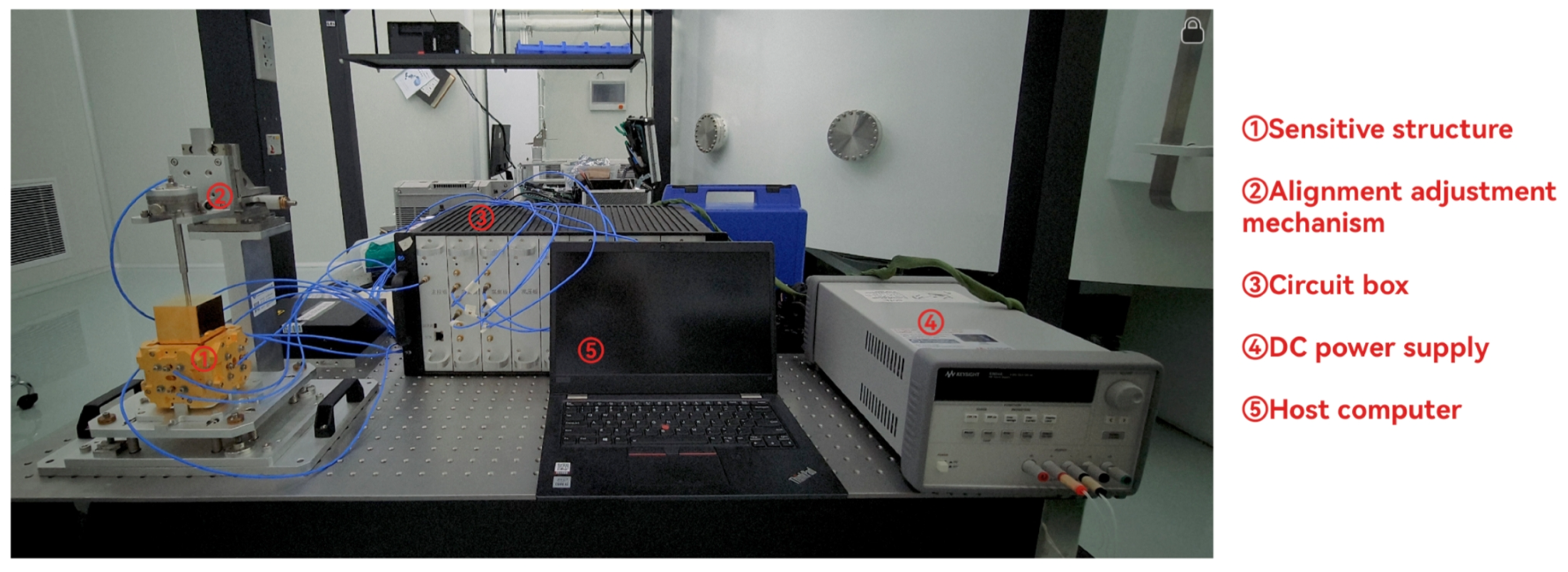
In this study, to accurately calibrate the gain coefficient, a single-axis, single-channel static calibration system was designed and implemented. The hardware configuration of this system is shown in Figure 4, mainly consisting of an alignment adjustment mechanism, a sensitive structure, a circuit box, a DC power supply, and a host computer.

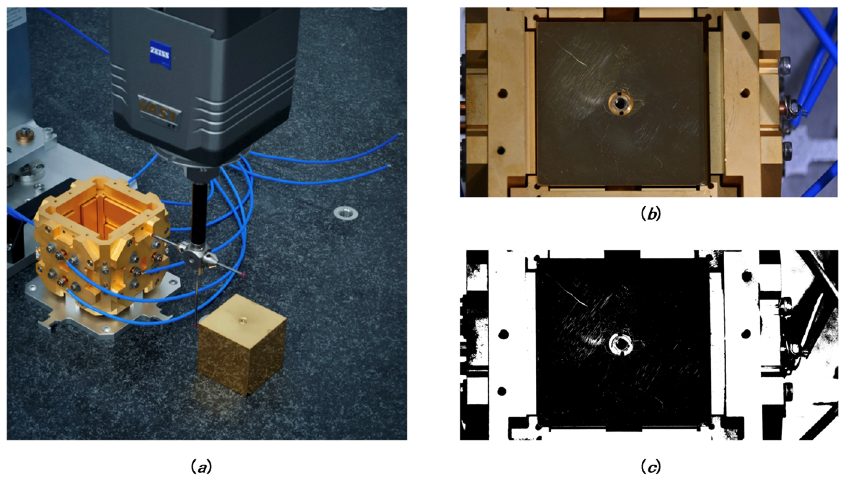
Figure 4. Photograph of the static single-axis calibration apparatus. Key components: (1) tilt/ translation/rotation alignment mechanism with locking screws; (2) sensitive structure (EH fixed on base, TM connected via rigid column); (3) circuit box; (4) DC power supply; (5) host computer. The TM geometry (46 mm side length) was pre-calibrated by CMM (±2 µm, $k=2$) to ensure SI traceability (see Figure 5c).

Figure 4. Photograph of the static single-axis calibration apparatus. Key components: (1) tilt/ translation/rotation alignment mechanism with locking screws; (2) sensitive structure (EH fixed on base, TM connected via rigid column); (3) circuit box; (4) DC power supply; (5) host computer. The TM geometry (46 mm side length) was pre-calibrated by CMM (±2 µm, $k=2$) to ensure SI traceability (see Figure 5c).

Figure 5. Image-based static displacement measurement workflow. (a) CMM measurement of the TM side length providing the SI-traceable dimensional reference; (b) raw high-resolution image (5120 × 5120) of the TM–EH gap acquired under diffused LED illumination; (c) binarized image after adaptive Canny edge extraction, serving as the input for Gaussian-integral subpixel edge detection and gap width determination.

Figure 5. Image-based static displacement measurement workflow. (a) CMM measurement of the TM side length providing the SI-traceable dimensional reference; (b) raw high-resolution image (5120 × 5120) of the TM–EH gap acquired under diffused LED illumination; (c) binarized image after adaptive Canny edge extraction, serving as the input for Gaussian-integral subpixel edge detection and gap width determination.

The alignment adjustment mechanism is the core component of this system. It consists of a tilt adjustment mechanism, a translation adjustment mechanism, and a rotation adjustment mechanism. The tilt adjustment mechanism is firmly installed on the base of the calibration bench, while the rotation and translation adjustment mechanisms are connected to the base via connecting arms. This mechanism allows for preliminary alignment and positioning of the relative position between the TM and EH along a single axis and can lock a specific displacement, providing a rigid static benchmark for the calibration method described in this study.

The sensitive structure consists of the EH and the TM. The EH is fixed on the base, while the TM is connected to the rotation adjustment mechanism via a rigid column. Electrode Tiles (ETs) are installed inside the electrode housing to sense the relative position between the EH and the TM. The required detection voltage for sensing is applied at the connection point between the rigid column and the rotation adjustment mechanism via a coaxial cable, and further applied to the TM. Each ET is connected to the sensing circuit inside the circuit box via coaxial cables, enabling real-time signal sensing.

This design not only improves the stability of the calibration process but also enhances the accuracy and reliability of the system by eliminating the vibration artifacts and thermal transients that are typically introduced by dynamic actuation platforms.

3.1.2. Calibration Scheme

Addressing the need for higher stability in gain coefficient parameter calibration for inertial sensor capacitive detection systems, this study proposes a static gain coefficient calibration method. The experimental setup uses a single-axis, single-channel electrode housing structure (X1 channel). The TM is fixed at an extreme displacement position $x_0=665\mathsf{\mu }$m by static geometric constraint (i.e., the TM is positioned at the extreme of its travel range within the EH and rigidly locked by the alignment mechanism). This parameter is determined by the geometric size difference between the electrode housing and the TM, compensated for machining tolerances.

The calibration displacement $x_0$ in this experiment was set to $665\mathsf{\mu }$m, resulting in $x_0/d_0\approx 0.665$. This ratio exceeds the range where the linear approximation is typically valid (usually requiring $x/d_0<0.1$), aiming to validate the method’s effectiveness under large-displacement scenarios such as the capture mode. Under this condition, the contributions of the higher-order terms $x^3/d_0^2$ and $x^5/d_0^4$ in Equation (3) to $\mathsf{\Delta }C$ are significant and must be considered. Consequently, the model incorporating these terms was employed in the calibration:

$$U_{dc}=K{U}_d\left(x+{\displaystyle \frac{x^3}{d_0^2}}+{\displaystyle \frac{x^5}{d_0^4}}\right)+U_0.$$

(11)

Setting $x=x_0$, the calculation formula for the gain coefficient is

$$K={\displaystyle \frac{U_{dc}-U_0}{U_d\left(x_0+{\displaystyle \frac{x_0^3}{d_0^2}}+{\displaystyle \frac{x_0^5}{d_0^4}}\right)}}.$$

(12)

Prior to the static calibration experiment, the TM side length (46 mm) was independently measured using a Coordinate Measuring Machine (CMM) to establish a traceable geometric reference. The CMM measurement, with an expanded uncertainty of $\pm 2\mathsf{\mu }$m ($k=2$), serves as the primary length standard for the pixel equivalent calibration in the image-based measurement system (see Section 4.1.1). This ensures that the displacement benchmark $x_0$ is ultimately traceable to the SI unit of length. The single-point validation at $x_0=665\mathsf{\mu }$m was deliberately chosen to stress-test the nonlinear model under the most challenging large-displacement condition.

In actual testing, the sensing voltage $U_{dc}$ can be read directly from the host computer platform, the detection voltage amplitude $U_d$ is selected manually, and the bias voltage $U_0$ can be determined using the forward/reverse connection testing technique.

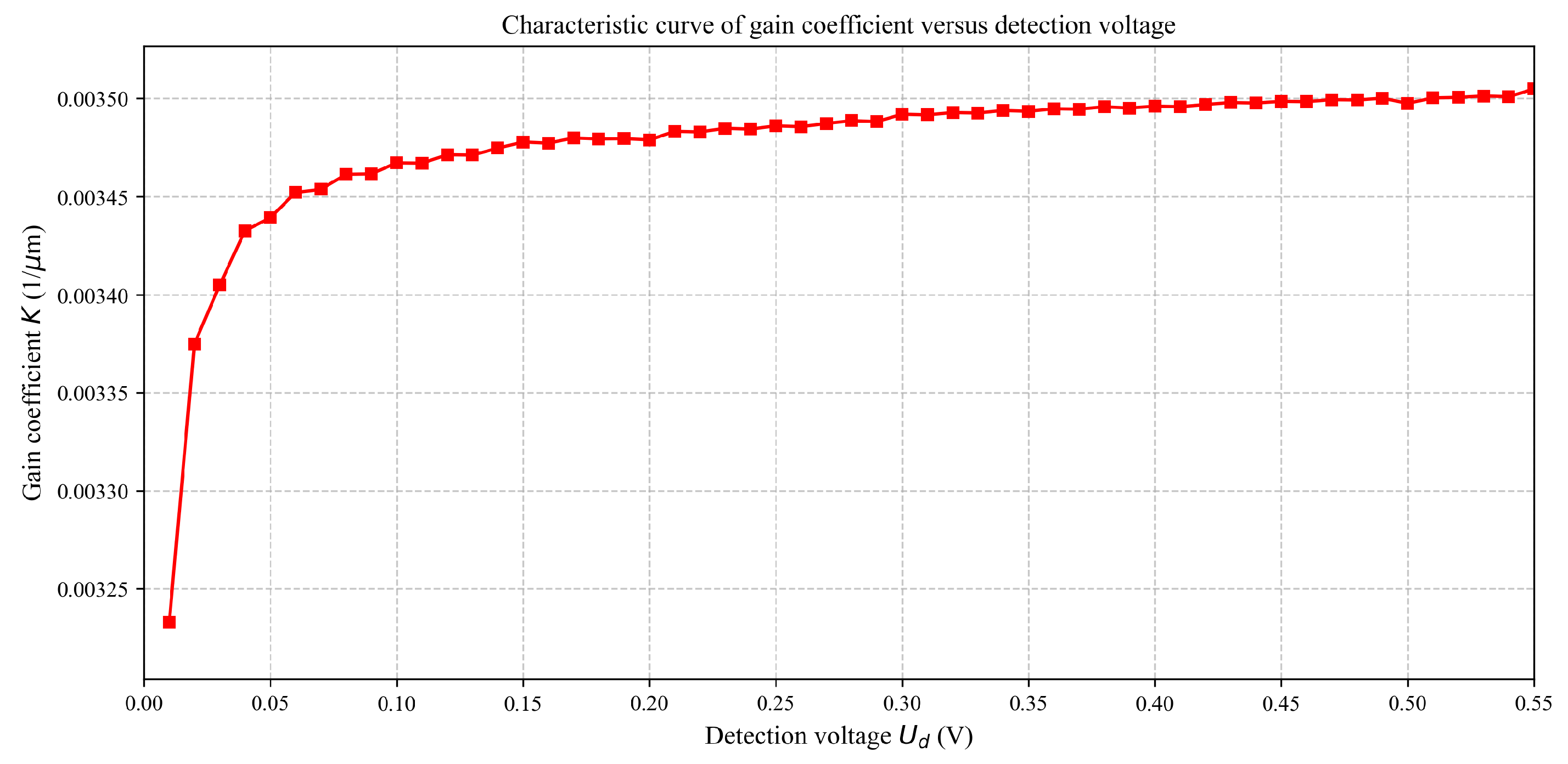
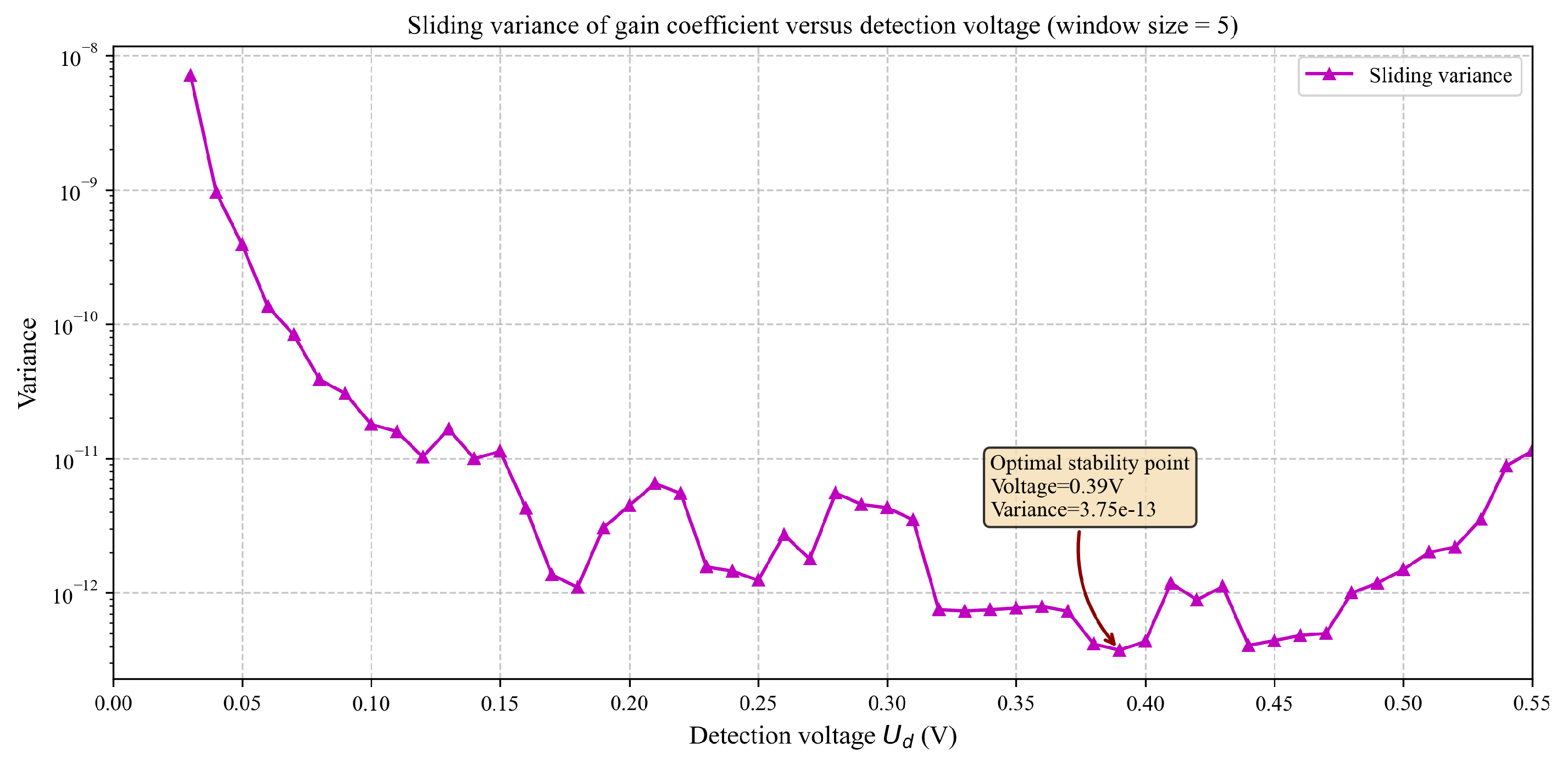
The proposed static approach serves as a complementary ground-based technique to traditional dynamic calibration methods (such as the piezoelectric platform sinusoidal motion mode). By eliminating moving actuators, it circumvents actuator-induced vibration artifacts, thereby providing a stable displacement benchmark particularly suited for high-stability gain calibration. As shown in Figure 6, the characteristic curve of the gain coefficient versus detection voltage is smooth and consistent, without significant fluctuations; the results of five consecutive tests in Figure 8 further show that the RMSPER of the gain coefficient is of only $0.01658$%, with minimal cumulative variance. This consistency highlights the effectiveness of the static method in providing a vibration-free reference for laboratory validation, alongside dynamic techniques that remain essential for in-orbit and multi-DoF scenarios. This design provides high repeatability of the calibration process, providing a reliable foundation for subsequent experiments.

Figure 6. Characteristic curve of the calibrated gain coefficient K versus detection voltage amplitude $U_d$. Experimental conditions: static displacement $x_0=665\mathsf{\mu }$m ($x_0/d_0\approx 0.665$), $U_d$ swept from 0.01 V to 0.55 V in 0.01 V steps, output voltage sampled at 10 Hz for 5 min per point, forward/reverse connection bias correction applied. The sliding-variance analysis is shown in Figure 7.

Figure 6. Characteristic curve of the calibrated gain coefficient K versus detection voltage amplitude $U_d$. Experimental conditions: static displacement $x_0=665\mathsf{\mu }$m ($x_0/d_0\approx 0.665$), $U_d$ swept from 0.01 V to 0.55 V in 0.01 V steps, output voltage sampled at 10 Hz for 5 min per point, forward/reverse connection bias correction applied. The sliding-variance analysis is shown in Figure 7.

Figure 7. Sliding variance (window size = 5) of the gain coefficient versus detection voltage amplitude, corresponding to the data in Figure 6. The variance is plotted on a logarithmic scale to resolve the extremely small dispersion (on the order of ${10}^{-13}$). The annotated optimal stability point indicates the detection voltage ($U_d\approx 0.39$ V) at which the gain coefficient exhibits minimal variance, supporting the independence of K on $U_d$ across the operating range. Experimental conditions identical to Figure 6.

Figure 7. Sliding variance (window size = 5) of the gain coefficient versus detection voltage amplitude, corresponding to the data in Figure 6. The variance is plotted on a logarithmic scale to resolve the extremely small dispersion (on the order of ${10}^{-13}$). The annotated optimal stability point indicates the detection voltage ($U_d\approx 0.39$ V) at which the gain coefficient exhibits minimal variance, supporting the independence of K on $U_d$ across the operating range. Experimental conditions identical to Figure 6.

3.1.3. Image-Based Displacement Measurement System

To quantify the static displacement benchmark $x_0$ without contact-induced deformation, a dedicated image-based measurement subsystem was integrated into the calibration apparatus. Its design rationale and hardware configuration are described as follows.

Hardware configuration. The imaging chain comprises a Touptek IUA25000KPA industrial CMOS camera (GMAX0505 sensor, 25 MP, 5120 × 5120 pixels, 1-inch optical format) and a Myutron FTV03C-110 bi-telecentric lens (0.28× magnification, distortion <0.1%). The bi-telecentric architecture ensures nearly constant magnification across the depth of field, effectively suppressing perspective distortion when imaging the TM–EH micro-gap. The camera is mounted perpendicularly above the sensitive structure, and images are captured under uniform, diffused LED illumination to minimize specular reflection from the gold-coated TM and EH surfaces.

Metrological traceability chain. The SI traceability is established in two stages: (i) the TM side length (46 mm) is independently measured by a CMM (±2 µm expanded uncertainty, $k=2$), providing a primary length standard; (ii) this CMM-calibrated dimension is used to determine the pixel equivalent P via subpixel edge detection, transferring the length standard to the image domain. The displacement benchmark $x_0$ is therefore traceable to the SI unit of length through a quantifiable, two-step calibration chain.

Subpixel edge detection algorithm. Pixel-level edges are first extracted using an adaptive Canny operator, followed by subpixel refinement based on Gaussian integral curve fitting along the normal direction of the edge gradient profile. Among subpixel edge detection methods—including moment-based (Zernike), polynomial fitting (Steger), and Gaussian integral approaches—each exhibits distinct characteristics under different imaging conditions. The Gaussian integral method was selected for this work because it demonstrates favorable robustness against illumination non-uniformity and edge-gradient asymmetry, which are frequently encountered in images of gold-coated TM and EH surfaces under diffused LED lighting. This selection is further supported by Yuan et al. [22], who reported that Gaussian-integral-based subpixel detection achieves reprojection errors below 0.06 pixels in telecentric imaging systems. Under the present experimental conditions, this algorithm achieves an edge localization repeatability of approximately 0.05 pixels (∼0.45 µm), contributing to a relative expanded uncertainty of approximately 0.3% for the static displacement benchmark.

3.2. Bias Voltage Test

Before validating the bias model, the circuit’s bias voltage must be accurately measured. This study adopts the forward/reverse connection bias voltage testing method, employing the calibration test equipment circuit box directly for the experiment.

The specific test scheme is as follows: First, connect the circuit box to the X1 path of the sensitive structure, where electrodes X1+ and X1– are connected to the two input terminals on the circuit box interface panel, respectively. This wiring configuration is defined as the forward connection. Then, swap the connections of the two input terminals, defined as the reverse connection. During this process, to minimize the stray capacitance changes caused by wiring changes, the number of forward/reverse connection swaps should be reduced as much as possible. In this experiment, we first collected the output voltage data under the forward connection, then collected the data under the reverse connection. Only one line exchange was required throughout the experiment.

The output voltage values were read and collected directly through the host computer platform. Assuming random noise is negligible, the output voltages $U_{+}$ and $U_{-}$ under forward and reverse connections can be expressed as

$$U_{+}=K{U}_d{\displaystyle \sum _{i=0}^{\infty }}{\displaystyle \frac{x^{2i+1}}{d_0^{2i}}}+U_0,$$

(13)

$$U_{-}=K{U}_d{\displaystyle \sum _{i=0}^{\infty }}{\displaystyle \frac{{(-x)}^{2i+1}}{d_0^{2i}}}+U_0.$$

(14)

From Equations (13) and (14), it follows that

$$U_0={\displaystyle \frac{U_{+}+U_{-}}{2}}.$$

(15)

4. Static Calibration Experiment

4.1. Gain Coefficient Calibration Experiment

4.1.1. Gain Coefficient Characteristic Test

This study conducted a calibration experiment for the X-axis single-axis, single-channel configuration. Before the experiment, the TM was first adjusted to the center of the EH using the alignment and fine-tuning controls described in Section 3 to perform zero calibration, ensuring the output sensing voltage from the host computer platform was zero at the center position. Using the fine-adjustment knobs of the alignment mechanism, the TM was positioned at an extreme position on one side of the EH. The displacement corresponding to this position is denoted as $x_0$, and the relative position between the TM and EH was fixed by locking the alignment mechanism’s locking screws.

The extreme displacement $x_0$ was quantified using the image-based measurement system detailed in Section 3.1.3. The CMM-calibrated TM side length (46 mm) served as the geometric reference for pixel-equivalent calibration. For each image acquisition, the subpixel edge detection algorithm located the boundaries of the TM and the EH inner wall, and the gap width was measured at five characteristic locations distributed along the gap. The entire image acquisition–processing–calculation cycle was repeated for 10 independent image sets captured at different times. The final calibrated value of $x_0$ was taken as the average of these measurements, yielding $x_0=665\mathsf{\mu }$m with a relative expanded uncertainty of approximately 0.3% ($k=2$).

An illustration of this image-based measurement procedure with CMM-calibrated geometric references is presented in Figure 5.

To ensure the statistical reliability of the measurement and to eliminate potential systematic errors, this entire process was repeated for multiple images taken at different times. The final calibrated value of $x_0$ was taken as the average of the results from these multiple measurement sets. This method effectively avoids the deformation errors and operational uncertainties that can be introduced by contact-based measurement techniques, providing a more robust and traceable displacement benchmark.

By relying on a rigid static geometric constraint rather than moving actuators, this method establishes a displacement benchmark free from actuator-induced nonlinearity, creep, and thermal drift. As a complementary ground-based technique to dynamic calibration, it is particularly valuable for achieving highly stable and repeatable static calibration in laboratory environments.

In the experiment, a host-computer platform was used to implement a continuously adjustable detection-voltage ($U_d$) scheme from 0.01 V to 0.55 V. The voltage was swept across the full range in 0.01 V steps, while the host PC acquired the output-voltage data at a sampling rate of 10 Hz for 5 min. Simultaneously, the forward-and-reverse wiring zero-bias method described in Section 3.2 was applied to measure both the positive and negative bias voltages, so that the zero-bias voltage for every detection voltage $U_d$ could be determined through Equation (15). Equation (12) then gives the measured gain coefficient, yielding the gain-coefficient-versus-detection-voltage characteristic curve shown in Figure 6. A sliding-variance analysis (window size = 5) of this curve is presented in Figure 7. The results demonstrate—consistent with the theoretical derivation in Section 2.3—that the gain coefficient is determined solely by the circuit-structure parameters and is independent of $U_d$ (sliding-variance values lie between ${10}^{-13}$), strongly supporting the constancy of the gain coefficient.

4.1.2. Gain Coefficient Calibration

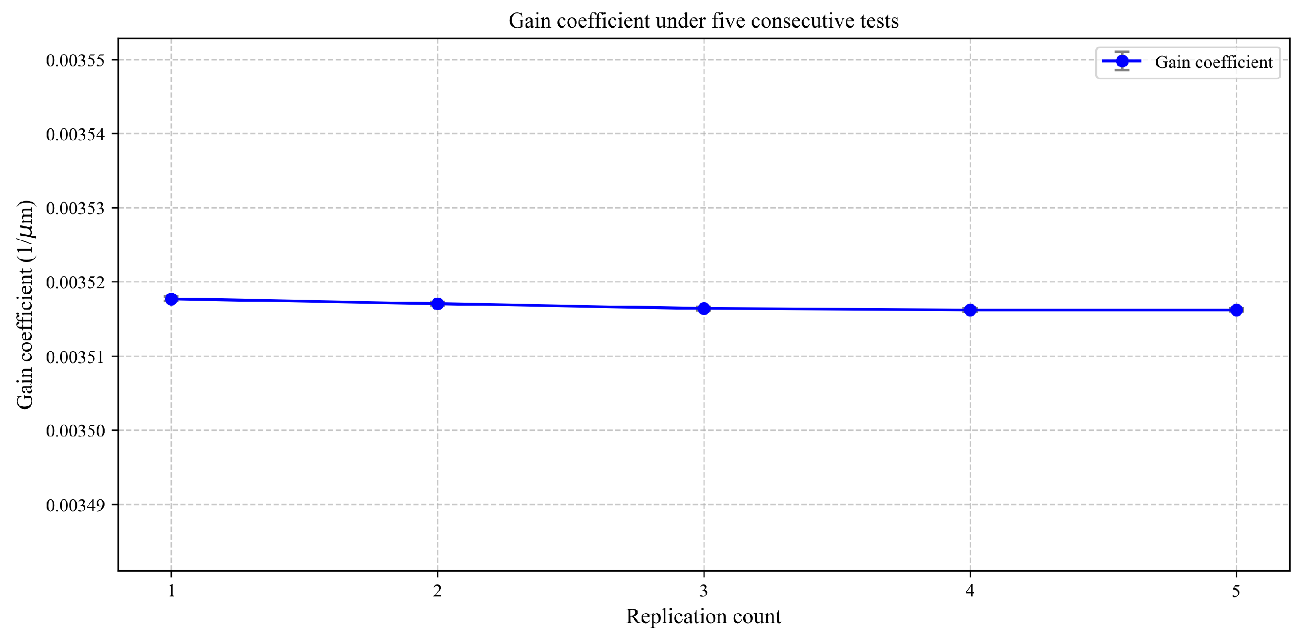
To verify the stability of the gain coefficient calibration scheme, the calibrated value of the gain coefficient was measured five times consecutively. The output voltage was collected via the host computer at a sampling frequency of 10 Hz for a sampling duration of 10 min. During the testing process, the detection voltage $U_d$ was optimally selected as 0.39 V [27]. The test values of the gain coefficient for these five groups were determined according to Equation (12), as shown in Figure 8.

The mean value, Root Mean Square Percentage Error (RMSPER), and cumulative variance of each group of data were calculated, as shown in

Table 3. Analysis of X1 channel gain coefficient calibration values.

Channel	Mean Gain Coefficient (1/µm)	Gain Coefficient RMSPER (%)	Cumulative Variance	Theoretical Gain Coefficient (1/µm)
X1	$3.5167\times {10}^{-3}$	0.01658	$3.3984\times {10}^{-13}$	$3.5128\times {10}^{-3}$

. The mean value of each group of data was taken as the calibrated value of the gain coefficient. It can be observed that the actual tested gain coefficient for each channel slightly differed from the theoretical value, primarily due to parameter variations in circuit components and machining errors of the sensitive structure. Meanwhile, the RMSPER of the results from the five tests was 0.01658%, verifying the feasibility and high stability of this calibration method. Furthermore, the result was achieved under a large displacement condition ($x_0/d_0\approx 0.665$), validating the accuracy of the model incorporating higher-order nonlinear terms (Equation (11)) adopted in this paper for such scenarios. For comparison, if the simplified linear model (i.e., Equation (4)) were used to process the same experimental data, the calculated gain coefficient would exhibit a deviation exceeding 5% from the theoretical value. This further underscores the necessity of accounting for nonlinear effects in large-displacement calibration.

4.2. Zero Bias Model Validation

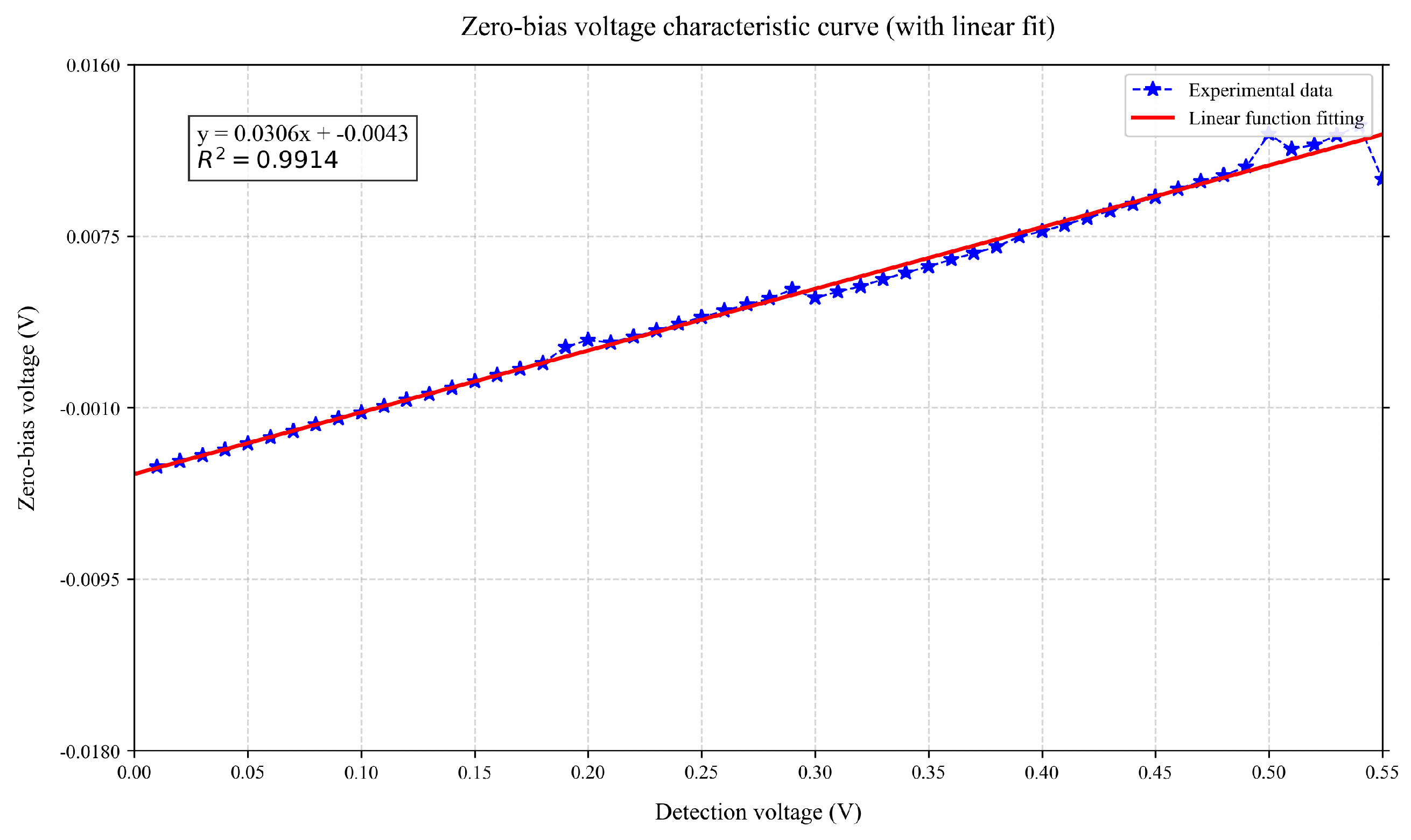
This study validated the zero bias model based on the testing method described in Section 3.2. According to the inference from Equation (9), the sensing voltage bias value has a linear relationship with $U_d$. The slope of its function is the bias coefficient, and the intercept is the fixed offset value. As described in Section 4.1, the bias voltage values under different detection voltage amplitudes were measured during the gain coefficient characteristic curve testing, resulting in the linear function fitting curve shown in Figure 9. It can be seen that the experimental fitting curve of bias voltage versus detection voltage amplitude matches well with the linear function, validating the circuit characteristic that the sensing voltage bias value has a linear relationship with $U_d$.

Limitations and Future Work

It is important to note that the present experimental validation is intentionally limited to a single-channel (X1), single-axis, and unidirectional configuration. This restriction arises from the current laboratory prototype, which was designed to demonstrate the feasibility of the proposed static benchmark concept rather than to provide a full multi-DoF characterization. Extension to multi-channel (X1–X6) and multi-axis (X, Y, Z) validation requires additional electrode routing, synchronized readout electronics, and a multi-axis alignment fixture, which are currently under assembly and will be reported in subsequent work. Nevertheless, the single-channel results already confirm the repeatability and traceability of the static calibration principle.

4.3. Uncertainty Analysis

To evaluate the reliability of this static calibration method, an uncertainty assessment of the gain coefficient calibration results was conducted following the Guide to the Expression of Uncertainty in Measurement (GUM). The focus of the analysis was on identifying and quantifying the significant contributing items affecting the results.

4.3.1. Identification of Uncertainty Sources

Based on the above theoretical framework and experiments, the main sources of uncertainty affecting the gain coefficient K were analyzed as follows:

• Measurement uncertainty of the static displacement gap ${\mathit{x}}_{\mathbf{0}}$: This is the primary limiting factor. It stems from the resolution and distortion of the image system, the subpixel accuracy of the image processing algorithm in edge detection (i.e., determining the boundaries of the TM and EH), the uncertainty in calculating the pixel equivalent $\mathit{P}$ (arising from the CMM-calibrated TM reference side length and its subpixel pixel measurement error in the image), and the statistical fluctuation from multiple measurements at different gap locations.
• Measurement uncertainty of the output voltage ${\mathit{V}}_{\mathrm{out}}$: Determined by the accuracy of the digital multimeter (DMM).
• Repeatability of the static calibration device: This item is the core indicator for assessing the inherent precision and stability of the method itself, directly evaluated through multiple repeated experiments.

4.3.2. Evaluation of Various Uncertainty Components

• Measurement uncertainty of static displacement gap ${\mathit{x}}_{\mathbf{0}}$, $\mathit{u}\mathbf{\left(}{\mathit{x}}_{\mathbf{0}}\mathbf{\right)}$
  • Evaluation method
    • Type B evaluation, synthesized from imaging system characteristics and subpixel algorithm performance.
  • Explanation and Calculation
    • The value of ${\mathit{x}}_{\mathbf{0}}$ is determined indirectly via the image-based measurement chain described in Section 3.1.3. The uncertainty budget comprises the following components:

      (a)

      Camera spatial resolution and telecentric lens distortion, ${\mathit{u}}_{\mathbf{1}}\mathbf{\left(}{\mathit{x}}_{\mathbf{0}}\mathbf{\right)}$: The GMAX0505 sensor has a physical pixel pitch of 2.5 µm; at the system magnification of 0.28×, the pixel equivalent is $\mathit{P}\mathbf{\approx }\mathbf{9.0}\mathsf{\mu }$m/pixel. The lens distortion is specified as <0.1%, contributing a geometric error bound of ±0.046 mm across the 46 mm field. Assuming a rectangular distribution, ${\mathit{u}}_{\mathbf{1}}\mathbf{\left(}{\mathit{x}}_{\mathbf{0}}\mathbf{\right)}\mathbf{\approx }\mathbf{0.027}\mathsf{\mu }$m, which is negligible compared to other sources.

      (b)

      Subpixel edge detection residual error, ${\mathit{u}}_{\mathbf{2}}\mathbf{\left(}{\mathit{x}}_{\mathbf{0}}\mathbf{\right)}$: The Gaussian integral fitting algorithm achieves a repeatability of 0.05 pixels under stable illumination [22,23], corresponding to ∼0.45 µm. Type B evaluation with rectangular distribution gives ${\mathit{u}}_{\mathbf{2}}\mathbf{\left(}{\mathit{x}}_{\mathbf{0}}\mathbf{\right)}=\mathbf{0.45}\mathbf{/}\sqrt{\mathbf{3}}\mathbf{\approx }\mathbf{0.26}\mathsf{\mu }$m.

      (c)

      Pixel equivalent calibration uncertainty, ${\mathit{u}}_{\mathbf{3}}\mathbf{\left(}{\mathit{x}}_{\mathbf{0}}\mathbf{\right)}$: The CMM calibration uncertainty of the TM side length (±2 µm, $\mathit{k}=\mathbf{2}$) corresponds to a standard uncertainty of $\mathbf{1}\mathsf{\mu }$m. Propagated through $\mathit{P}=\mathbf{46}\mathbf{mm}\mathbf{/}{\mathit{N}}_{\mathbf{TM}}$ together with the subpixel pixel-counting error of ${\mathit{N}}_{\mathbf{TM}}$ (±0.05 pixels), this yields a relative standard uncertainty of approximately 0.005% for $\mathit{P}$, translating to ${\mathit{u}}_{\mathbf{3}}\mathbf{\left(}{\mathit{x}}_{\mathbf{0}}\mathbf{\right)}\mathbf{\approx }\mathbf{0.03}\mathsf{\mu }$m.

      (d)

      Gap measurement repeatability, ${\mathit{u}}_{\mathbf{4}}\mathbf{\left(}{\mathit{x}}_{\mathbf{0}}\mathbf{\right)}$: From 10 independent image acquisitions, each with 5 spatial sampling points along the gap, the pooled standard deviation of the mean gap measurement is ${\mathit{s}}_{\mathbf{gap}}=\mathbf{0.95}\mathsf{\mu }$m; thus ${\mathit{u}}_{\mathbf{4}}\mathbf{\left(}{\mathit{x}}_{\mathbf{0}}\mathbf{\right)}={\mathit{s}}_{\mathbf{gap}}\mathbf{\approx }\mathbf{0.95}\mathsf{\mu }$m. This component encapsulates residual illumination fluctuations, edge gradient variations, and algorithm noise.

      Taken together, as these components are uncorrelated, the combined standard uncertainty of ${\mathit{x}}_{\mathbf{0}}$ is

      $$\mathit{u}\mathbf{\left(}{\mathit{x}}_{\mathbf{0}}\mathbf{\right)}=\sqrt{{\mathit{u}}_{\mathbf{1}}{\mathbf{\left(}{\mathit{x}}_{\mathbf{0}}\mathbf{\right)}}^{\mathbf{2}}+{\mathit{u}}_{\mathbf{2}}{\mathbf{\left(}{\mathit{x}}_{\mathbf{0}}\mathbf{\right)}}^{\mathbf{2}}+{\mathit{u}}_{\mathbf{3}}{\mathbf{\left(}{\mathit{x}}_{\mathbf{0}}\mathbf{\right)}}^{\mathbf{2}}+{\mathit{u}}_{\mathbf{4}}{\mathbf{\left(}{\mathit{x}}_{\mathbf{0}}\mathbf{\right)}}^{\mathbf{2}}}$$

      (16)

      $$\mathit{u}\mathbf{\left(}{\mathit{x}}_{\mathbf{0}}\mathbf{\right)}\approx \sqrt{{\mathbf{0.027}}^{\mathbf{2}}+{\mathbf{0.26}}^{\mathbf{2}}+{\mathbf{0.03}}^{\mathbf{2}}+{\mathbf{0.95}}^{\mathbf{2}}}\mathbf{\approx }\mathbf{0.99}\mathsf{\mu }\mathrm{m}.$$

      (17)
      The corresponding relative standard uncertainty is $\mathit{u}\mathbf{\left(}{\mathit{x}}_{\mathbf{0}}\mathbf{\right)}\mathbf{/}{\mathit{x}}_{\mathbf{0}}\mathbf{\approx }\mathbf{0.99}\mathbf{/}\mathbf{665}\mathbf{\approx }\mathbf{0.15}$%. Using a coverage factor $\mathit{k}=\mathbf{2}$, the estimated relative expanded uncertainty is ${\mathit{u}}_{\mathbf{rel}}\mathbf{\left(}{\mathit{x}}_{\mathbf{0}}\mathbf{\right)}\mathbf{\approx }\mathbf{0.3}$%, consistent with the empirical repeatability observed in this work. The dominant contribution arises from the gap measurement repeatability (${\mathit{u}}_{\mathbf{4}}$), which reflects the present implementation of the optical setup and is amenable to reduction through higher-grade CMM calibration, active illumination control, or increased sampling.
• Measurement uncertainty of output voltage ${\mathit{V}}_{\mathbf{out}}$, $\mathit{u}\mathbf{\left(}{\mathit{V}}_{\mathbf{out}}\mathbf{\right)}$
  • Evaluation method
    • Type B evaluation.
  • Explanation and Calculation
    • According to its technical manual, the digital multimeter used in this experiment has an accuracy specification of $\pm (\mathbf{0.05}\mathbf{\%}\mathrm{of}\mathrm{Reading}+\mathbf{2}\mathrm{Digits})$ in the 2 V range. When the measured value ${\mathit{V}}_{\mathbf{out}}\mathbf{\approx }\mathbf{2.5}$ V, the maximum permissible error is $\mathbf{2.5}\mathbf{V}\times \mathbf{0.05}\mathbf{\%}+\mathbf{0.002}\mathbf{V}\mathbf{\approx }\mathbf{0.00325}\mathbf{V}$. Assuming a rectangular distribution, its standard uncertainty is:

      $$\mathit{u}\mathbf{\left(}{\mathit{V}}_{\mathbf{out}}\mathbf{\right)}={\displaystyle \frac{\mathbf{0.00325}\mathbf{V}}{\sqrt{\mathbf{3}}}}\mathbf{\approx }\mathbf{0.00188}\mathbf{V}.$$

      (18)
• Uncertainty introduced by static calibration repeatability, ${\mathit{u}}_{\mathbf{repeat}}\left(\mathit{K}\right)$
  • Evaluation method
    • Type A evaluation.
  • Explanation and Calculation
    • This component is directly evaluated from the data of the 5 repeatability experiments, quantifying the inherent random error of the method. As shown in Figure 8, the results of the 5 measurements show high consistency. Their standard deviation is calculated as the standard uncertainty:

      $${\mathit{u}}_{\mathbf{repeat}}\mathbf{\left(}\mathit{K}\mathbf{\right)}=\mathit{s}\mathbf{\left(}\mathit{K}\mathbf{\right)}=\mathbf{5.82}\times {\mathbf{10}}^{-\mathbf{7}}\mathbf{1}/\mathsf{\mu }\mathrm{m}.$$

      (19)
      Its relative value is extremely low, about 0.0166%. The extremely low dispersion is indicative of the high stability of the static method.

4.3.3. Combined Standard Uncertainty Calculation and Final Report

The combined standard uncertainty of the gain coefficient K is synthesized from the above three components. The contribution of the sensing system’s inherent noise term to the combined result is considered negligible and is ignored in the calculation.

$${\displaystyle \frac{u_c\left(K\right)}{K}}\approx \sqrt{{\left({\displaystyle \frac{u\left(V_{\mathrm{out}}\right)}{V_{\mathrm{out}}}}\right)}^2+{\left({\displaystyle \frac{u\left(x_0\right)}{x_0}}\right)}^2+{\left({\displaystyle \frac{u_{\mathrm{repeat}}\left(K\right)}{K}}\right)}^2}.$$

(20)

Substituting the calculated values yields

$${\displaystyle \frac{u_c\left(K\right)}{K}}\approx \sqrt{{\left(0.00075\right)}^2+{\left(0.003\right)}^2+{\left(0.000166\right)}^2}\approx 0.0031.$$

(21)

Furthermore:

$$u_c\left(K\right)=K\times 0.0031\approx 1.09\times {10}^{-5}1/\mathsf{\mu }\mathrm{m}.$$

(22)

Using a coverage factor $k=2$ (approximately 95% confidence level), the expanded uncertainty is

$$U\left(K\right)=2\times u_c\left(K\right)\approx 2.18\times {10}^{-5}1/\mathsf{\mu }\mathrm{m}.$$

(23)

Therefore, the calibration result can be reported as

$$K=(351.67\pm 2.18)\times {10}^{-5}1/\mathsf{\mu }\mathrm{m}.$$

(24)

4.3.4. Analysis and Discussion

The uncertainty analysis presented above allows for a critical evaluation of the proposed static calibration method. The following observations can be made:

• Dominant Uncertainty Source: The combined standard uncertainty of the gain coefficient K is currently dominated by the measurement uncertainty of the static displacement gap $x_0$, $u\left(x_0\right)$. As derived in Section 4.3, the relative contribution of $u\left(x_0\right)$ to the overall uncertainty budget exceeds 90%, while the contributions from the output voltage measurement ($u\left(V_{\mathrm{out}}\right)$) and the method repeatability ($u_{\mathrm{repeat}}\left(K\right)$) are substantially smaller. This indicates that under the current experimental conditions, the accuracy of the calibration is primarily limited by the precision of the image-based gap measurement technique employed. The specific factors contributing to $u\left(x_0\right)$ include the CMM traceability uncertainty, the subpixel edge detection residual error, and the illumination stability during image acquisition. Consequently, the total expanded uncertainty ($U\approx 2.18\times {10}^{-5}1/\mathsf{\mu }$m) reflects the present implementation of the optical measurement setup rather than an inherent limitation of the static calibration principle itself.
• Inherent Method Stability: Despite the relatively large contribution from $u\left(x_0\right)$, the repeatability of the method, quantified by $u_{\mathrm{repeat}}\left(K\right)/K=0.0166$%, is exceptionally low. This high repeatability demonstrates that the static approach provides a highly stable and reproducible displacement reference. Once the gap $x_0$ is accurately characterized, the subsequent gain coefficient determination is consistent across multiple trials, confirming that the method is robust against random variations in the experimental procedure. This inherent stability is a key advantage of the static calibration concept.
• Complementary Role to Dynamic Methods: The proposed static method is intended as a ground-based complement to dynamic calibration techniques, not as their replacement. While dynamic methods remain indispensable for in-orbit and multi-DoF characterization, they introduce uncertainty sources associated with piezoelectric actuators or precision displacement stages, such as mechanical vibrations, actuator nonlinearity, hysteresis, and thermal drift. The present static approach circumvents these particular error sources by transforming the calibration task into a well-defined geometric measurement problem, where the primary uncertainty stems from a single, quantifiable source (the determination of $x_0$). In this way, the two approaches address different operational needs: dynamic methods excel in flight-representative scenarios, whereas the static method provides a vibration-free, SI-traceable benchmark for high-stability laboratory validation.
• Path for Accuracy Improvement: The analysis clearly identifies that reducing the uncertainty in $x_0$ would directly and substantially improve the overall calibration accuracy. This could be achieved through several practical enhancements: employing higher-resolution cameras, utilizing telecentric lenses with lower distortion, further improving the CMM calibration uncertainty of the TM geometry (e.g., using higher-grade CMMs or multiple measurement averaging), and performing rigorous camera calibration to correct for optical aberrations. With such improvements, the relative uncertainty in $x_0$ could potentially be reduced by an order of magnitude or more, thereby bringing the total calibration uncertainty closer to the method’s intrinsic repeatability limit.

In summary, the uncertainty analysis indicates that while the current calibration accuracy is constrained by the image-based measurement of the static gap, the proposed static method exhibits high repeatability and effectively eliminates complex dynamic error sources. The dominant uncertainty component is clearly identified and quantifiable, providing a direct and feasible pathway for future accuracy improvements.

5. Conclusions

This paper has presented and validated a high-precision static calibration method for inertial sensor capacitive sensing, based on image-based displacement measurement and bias modeling. The method introduces three key contributions: (i) a static displacement benchmark established by a high-precision image-based measurement system, utilizing CMM-calibrated geometric references (46 mm TM side length, ±2 µm expanded uncertainty, $k=2$) and subpixel edge detection to provide SI-traceable quantification, thereby eliminating the vibration-induced instability inherent in dynamic calibration; (ii) a nonlinear calibration model incorporating higher-order terms ($x^3/d_0^2$ and $x^5/d_0^4$) to address the significant nonlinear errors in large-displacement scenarios such as capture mode; and (iii) a composite bias model that successfully separates the detection-voltage-dependent component (${\delta }_0{U}_d$) from the fixed offset ($u_c$). These three elements collectively contribute to addressing the critical challenges identified in Section 1, mechanical vibration artifacts, bias voltage separation, and large-displacement nonlinearity, while establishing a complete metrological traceability chain essential for space gravitational wave detection missions. The main conclusions are as follows:

• SI-traceable image-based displacement benchmark: A non-contact image-based measurement technique was established as the core displacement quantification method. By combining a CMM-calibrated geometric reference (46 mm TM side length, ±2 µm expanded uncertainty, $k=2$), a high-resolution industrial camera (Touptek IUA25000KPA, 25 MP, 5120 × 5120), a bi-telecentric lens (Myutron FTV03C-110, 0.28× magnification), and a Gaussian-integral subpixel edge detection algorithm (0.05-pixel repeatability), the static displacement benchmark $x_0$ achieves a relative expanded uncertainty of approximately 0.3% ($k=2$). This demonstrates that image-based measurement can serve as a viable, traceable complement to mechanical displacement stages in high-precision static calibration, particularly for scenarios where mechanical stability and non-contact quantification are required.
• High stability and repeatability: Five consecutive calibration tests on the X1 channel yielded a gain coefficient RMSPER of only 0.01658%, confirming the effectiveness of the static method in suppressing mechanical noise. The reliability of this calibration is underpinned by the image-based displacement measurement technique, which provides a traceable quantification of the static displacement gap free from contact-induced errors. Uncertainty analysis further reveals that the method’s repeatability ($u_{\mathrm{repeat}}\left(K\right)/K=0.0166$%) is exceptionally good, with the overall accuracy currently limited primarily by the image-based gap measurement—a clearly identified pathway for future improvement.
• Validated composite bias model: Experimental results closely match the theoretical derivation, confirming that the bias voltage comprises both a dynamic component proportional to the detection voltage and a fixed offset. This provides a rigorous basis for quantitatively analyzing circuit asymmetry effects and correcting them in practical applications.

By combining the stability of a static geometric constraint with accurate bias modeling, this work establishes a simple yet reliable static calibration technique. We emphasize that the proposed method is intended to serve as a complementary ground-based tool to existing dynamic calibration approaches: it provides a vibration-free, SI-traceable displacement benchmark for high-stability gain validation in laboratory environments, while dynamic methods remain indispensable for in-orbit and multi-degree-of-freedom characterization. The underlying principle—using a CMM-traceable image-based benchmark for static calibration—offers a valuable reference for other high-precision displacement measurement systems where mechanical vibration presents a concern. Future work will focus on extending this static method to multi-axis coupling calibration and developing automated positioning structures for rapid multi-channel validation.

References

1. Dolesi, R.; Bortoluzzi, D.; Bosetti, P.; Carbone, L.; Cavalleri, A.; Cristofolini, I.; DaLio, M.; Fontana, G.; Fontanari, V.; Foulon, B.; et al. Gravitational sensor for LISA and its technology demonstration mission. Class. Quantum Grav. 2003, 20, S99–S108. [Google Scholar] [CrossRef]
2. Hu, W.R.; Wu, Y.L. The Taiji program in space for gravitational wave physics and the nature of gravity. Natl. Sci. Rev. 2017, 4, 685–686. [Google Scholar] [CrossRef]
3. Luo, Z.R.; Zhang, M.; Jin, G.; Wu, Y.; Hu, W. Introduction of Chinese space-borne gravitational wave detection program “Taiji” and “Taiji-1” satellite mission. J. Deep Space Explor. 2020, 7, 3–10. (In Chinese) [Google Scholar]
4. Luo, J.; Chen, L.S.; Duan, H.Z.; Gong, Y.G.; Hu, S.; Ji, J.; Liu, Q.; Mei, J.; Milyukov, V.; Sazhin, M.; et al. TianQin: A space-borne gravitational wave detector. Class. Quantum Grav. 2016, 33, 035010. [Google Scholar] [CrossRef]
5. Armano, M.; Audley, H.; Auger, G.; Baird, J.; Bassan, M.; Binetruy, P.; Born, M.; Bortoluzzi, D.; Brandt, N.; Caleno, M.; et al. Capacitive sensing of test mass motion with nanometer precision over millimeter-wide sensing gaps for space-borne gravitational reference sensors. Phys. Rev. D 2017, 96, 062004. [Google Scholar] [CrossRef]
6. Flury, J.; Bettadpur, S.; Tapley, B.D. Precise accelerometry onboard the GRACE gravity field satellite mission. Adv. Space Res. 2008, 42, 1414–1423. [Google Scholar] [CrossRef]
7. Touboul, P.; Foulon, B.; Christophe, B.; Marque, J.P. CHAMP, GRACE, GOCE instruments and beyond. In Intemational Association of Geodesy Symposia; Springer: Berlin/Heidelberg, Germany, 2012; pp. 215–221. [Google Scholar] [CrossRef]
8. Liorzou, F.; Touboul, P.; Rodrigues, M.; Métris, G.; Andre, Y.; Bergé, J.; Boulanger, D.; Bremer, S.; Chhun, R.; Christophe, B.; et al. MICROSCOPE instrument description and validation. Class. Quantum Grav. 2022, 39, 204002. [Google Scholar] [CrossRef]
9. Touboul, P.; Bernard, A. Electrostatic accelerometers for the Equivalence Principle test in space. Adv. Space Res. 2003, 32, 1357–1360. [Google Scholar] [CrossRef]
10. Ross, M.P.; Venkateswara, K.; Hagedorn, C.A.; Leupold, C.J.; Forsyth, P.W.F.; Wegner, J.D.; Shaw, E.A.; Lee, J.G.; Gundlach, J.H. A low-frequency torsion pendulum with interferometric readout. Rev. Sci. Instrum. 2021, 92, 054502. [Google Scholar] [CrossRef] [PubMed]
11. Wang, S.; Liu, H.; Dai, L.; Luo, Z.; Xu, P.; Li, P.; Gao, R.; Li, D.; Qi, K. Using DWS Optical Readout to Improve the Sensitivity of Torsion Pendulum. Sensors 2023, 23, 8087. [Google Scholar] [CrossRef] [PubMed]
12. Yang, F.; Bai, Y.; Hong, W.; Li, H.; Liu, L.; Sumner, T.J.; Yang, Q.; Zhao, Y.; Zhou, Z. Investigation of charge management using UV LED device with a torsion pendulum for TianQin. Class. Quantum Grav. 2020, 37, 115005. [Google Scholar] [CrossRef]
13. Wang, C.; Bai, Y.; Hu, M.; Li, D.; Li, K.; Ouyang, C.; Qu, S.; Xiao, C.; Yang, X.; Zhou, A.; et al. Development and experimental investigation of a high-precision capacitive displacement transducer of the inertial sensor for TianQin. Class. Quantum Gravity 2023, 40, 205010. [Google Scholar] [CrossRef]
14. Wang, S.X. Research on the Construction of the Sensitive Structure and Ground Evaluation Method of Space Inertial Sensor. Ph.D. Dissertation, Changchun Institute of Optics, Fine Mechanics and Physics, Chinese Academy of Sciences, Changchun, China, 2020. [Google Scholar]
15. Bai, Y.-z.; Zhou, Z.-b.; Tu, H.-b.; Wu, S.-c.; Cai, L.; Liu, L.; Luo, J. Capacitive position measurement for high-precision space inertial sensor. Front. Phys. China 2009, 4, 205–208. [Google Scholar] [CrossRef]
16. Li, H.; Li, G.; Hong, W.; Chen, B.; Chu, L.; Zhao, M.; Xiao, C.; Jia, B.; Bai, Y.; Zhou, Z. Capacitive sensing-based charge measurement for space inertial sensors. IEEE Trans. Instrum. Meas. 2024, 73, 6501509. [Google Scholar] [CrossRef]
17. Ge, C.; Zhang, D.F.; Li, P.Z.; Guo, K.; Li, P.Y.; Yang, H.J. Linearity calibration and uncertainty evaluation of capacitive displacement sensor. Opt. Precis. Eng. 2015, 23, 2546–2552. (In Chinese) [Google Scholar] [CrossRef]
18. Fichter, W.; Ziegler, T.; Vitale, S. Calibration methods for the LISA pathfinder drag-free system and expected performance. AIP Conf. Proc. 2006, 873, 675–681. [Google Scholar] [CrossRef]
19. Gan, L.; Mance, D.; Zweifel, P. LTP is FEE sensing channel: Front-end modeling and symmetry adjustment method. IEEE Sens. J. 2011, 12, 1071–1077. [Google Scholar] [CrossRef]
20. Li, S.; Zhao, P.; Sun, W. Structural design and static calibration of six-axis force/torque sensor. J. Phys. Conf. Ser. 2023, 2557, 012075. [Google Scholar] [CrossRef]
21. Yang, F.; Kong, D.; Wang, F.; Kong, L. A traceable dynamic calibration research of the measurement system based on quasi-static and dynamic calibration for accurate blast overpressure measurement. Meas. Sci. Technol. 2019, 30, 025005. [Google Scholar] [CrossRef]
22. Yuan, J.; Lin, H.; Shi, Z.; Wang, X.; Yang, G. Telecentric imaging calibration via integrated sub-pixel edge detection and illumination compensation. Opt. Precis. Eng. 2025, 33, 2578–2591. [Google Scholar] [CrossRef]
23. Lou, Q.; Lü, J.; Wen, L.; Xiao, J.; Zhang, G.; Hou, X. High-precision camera calibration method based on sub-pixel edge detection. Acta Opt. Sin. 2022, 42, 2012002. [Google Scholar] [CrossRef]
24. Moru, D.K.; Borro, D. A machine vision algorithm for quality control inspection of gears. Int. J. Adv. Manuf. Technol. 2019, 104, 1859–1872. [Google Scholar] [CrossRef]
25. Steger, C. An unbiased detector of curvilinear structures. IEEE Trans. Pattern Anal. Mach. Intell. 1996, 20, 113–125. [Google Scholar] [CrossRef]
26. Tabatabai, A.J.; Mitchell, O.R. Edge location to subpixel values in digital imagery. IEEE Trans. Pattern Anal. Mach. Intell. 1990, 12, 229–251. [Google Scholar] [CrossRef]
27. Mance, D. Development of Electronic System for Sensing and Actuation of Test Mass of the Inertial Sensor LISA Razvoj Elektroniskog Sustava za Ocitavanje i Pokretanje Test Mase Inercijalnog Senzora LISA; University of Split: Split, Croatia, 2012. [Google Scholar]
Figure 1. Modular architecture of the capacitive sensing circuit. (1) Differential capacitance formed by TM–EH electrode pairs; (2) Differential Capacitance Amplifier (DCA) for current-to-voltage conversion; (3) Bandpass Filter (BPF) at the 100 kHz carrier frequency; (4) phase-sensitive demodulator (multiplier + LPF) extracting the baseband displacement signal; (5) 100 kHz sinusoidal carrier and TTL reference; (6) ADC digitization. The signal path is indicated by solid arrows.
Instruments 10 00038 g001
Figure 2. Equivalent circuit of the sensing bridge viewed from the preamplifier input. The bridge is modeled as a voltage source U ˜ B R in series with source impedance Z B R . The secondary short-circuit condition ( U S = 0 ) used for impedance measurement is indicated.
Instruments 10 00038 g002
Figure 3. Principle of differential capacitive displacement sensing. (a) Schematic of the TM–EH assembly; (b) symmetric electrode configuration at zero displacement ( x = 0 ) with nominal gap d 0 ; (c) displaced configuration ( x 0 ) showing the asymmetric gap distances d 0 x and d 0 + x that produce the differential capacitance change Δ C .
Instruments 10 00038 g003
Figure 8. Gain coefficient obtained from five consecutive independent tests under identical static conditions. Experimental conditions: x 0 = 665 µ m, U d = 0.39 V, duration 10 min per test (sampled at 10 Hz). Error bars represent the standard deviation of the 10 min continuous data within each test; they are visually imperceptible (on the order of 10 7 1/µm) due to the high intrinsic stability of the static method. The RMSPER across the five tests is 0.01658%.
Instruments 10 00038 g008
Figure 9. Experimental validation of the composite bias model. Bias voltage U 0 (mean of forward and reverse connections) versus detection voltage amplitude U d . Experimental conditions: x 0 = 665 µ m, U d range 0.01–0.55 V. Linear fit: U 0 = 0.0306 U d 0.0043 with R 2 = 0.9914 , consistent with the linear dependence of bias on detection voltage predicted by Equation (10).
Instruments 10 00038 g009