Machine Learning-Driven Beam Tuning Using Adaptive Region Bayesian Optimization at INFN-LNL ^†

Abstract

Machine Learning (ML) techniques are increasingly being adopted in particle accelerator operations to enable efficient control of complex systems. At INFN–LNL, we investigated both offline and real-time ML-driven approaches to enhance beam quality, reduce setup time, and improve reliability across different accelerator facilities. As part of this effort, we developed Adaptive Region Bayesian Optimization (ARBO), a custom Bayesian Optimization algorithm that dynamically expands its search domain when the predicted optimum approaches a boundary. Offline studies applied ARBO to the design optimization of the medium-energy beam transport line of the ANTHEM BNCT facility. Real-time online tests demonstrated the effectiveness of ARBO. At PIAVE–ALPI, the combined transmission improved from 44.2% to 52.6%, corresponding to an ALPI-only increase from approximately 69% to 82%, approaching the theoretical maximum of 93%. At the ESS normal-conducting linac, ARBO enabled the simultaneous tuning of more than 50 control elements while improving transmission and maintaining stable trajectory correction. These results indicate that adaptive optimization strategies can substantially improve accelerator performance and support future advances in ML-assisted accelerator operations.

1. Introduction

Particle accelerators are complex machines that accelerate charged particles for research and applications in a variety of fields, ranging from particle and nuclear physics to medical applications. The design and operation of such machines require solving optimization problems involving the precise control of multiple parameters in order to maximize performance, efficiency, and availability. In addition, the design of future accelerators requires the use of increasingly nonlinear accelerator elements to meet performance goals while balancing cost and practical constraints [1,2]. Various numerical algorithms have been employed in the past, most of which are based on heuristic methods, notably the Nelder–Mead simplex algorithm [3,4] and the robust conjugate direction search (RCDS) [5], which rely heavily on extensive simulations and operator experience. However, even with the support of this algorithm and expert personnel, the design and operation of accelerators still involve long setup times due to the large number of accelerator components that must be optimized.

Recent advancements in optimization algorithms and artificial intelligence have enabled the exploration and solution of increasingly challenging optimization problems. One of the most promising and widely used algorithms in this field is Bayesian Optimization (BO) [6,7,8,9,10,11], owing to its flexibility, low initialization cost, and fast convergence. BO derives its operating principle from statistical Bayesian inference and is typically applied to black-box functions that are expensive to evaluate [12]. It constructs a probabilistic surrogate model, commonly a Gaussian process (GP) [13], to approximate the objective function and quantify uncertainty. An acquisition function is then used to iteratively select evaluation points, effectively balancing exploration and exploitation. This strategy enables efficient identification of optimal parameters with relatively few evaluations. However, the efficiency of BO in identifying the global optimum is generally limited to problems with fewer than approximately 20 dimensions and degrades significantly for higher-dimensional systems.

To address this limitation, several extensions of BO have been proposed. Among them, Trust Region Bayesian Optimization (TuRBO) [14] has gained attention for high-dimensional problems. TuRBO improves scalability by restricting the search to a localized region of the parameter space known as trust region (TR), which is centered around the most promising solution. The size of the TR is adapted during the optimization process, expanding when progress is observed and contracting otherwise. This strategy focuses computational effort on relevant areas of the search space, enabling more efficient exploration–exploitation trade-offs and faster convergence in high-dimensional settings compared to standard BO. TuRBO has already been successfully applied in accelerator physics, for example at the ESRF-EBS storage ring, where it was used to tune a subset of 24 sextupoles and 4 octupoles, selected from a total of 192 sextupoles and 64 octupoles, to optimize beam lifetime [15].

These successful demonstrations typically rely on a reduced set of tuning parameters, while full-scale accelerator optimization problems remain significantly higher-dimensional and constrained, particularly for high-energy or high-intensity machines. To address this challenge, the optimization problem can be constrained by incorporating beam-physics knowledge and by developing optimization strategies tailored to practical operational constraints. With these modifications to the basic BO framework, it is possible to leverage the strengths of the algorithm and extend its applicability to routine accelerator operations as well as high-performance optimization tasks in simulation studies.

In this work, a modified version of BO developed at INFN-LNL, referred to as Adaptive Region Bayesian Optimization (ARBO), is tested on various linear accelerator facilities in both simulation and operational settings. First, the working principle of the algorithm is described, highlighting the additional features that enable dynamic expansion of the search region as well as a comparison with vanilla BO and TuRBO. Subsequently, a series of offline and online case studies across different accelerator facilities are presented, detailing the optimization problems, objectives, and strategies employed for each system. The facilities investigated in this study include the ANTHEM-BNCT (Advanced Technologies for Human-centered Medicine-Boron Neutron Capture Therapy) facility, the INFN-LNL TAP (TANDEM-ALPI-PIAVE) accelerator complex, and ESS (European Spallation Source). Section 2 describes the materials and methodologies, Section 3 presents the performance and results achieved by the ARBO algorithm, and Section 4 discusses the implications of these findings.

2. Materials and Methods

2.1. Working Principle of ARBO

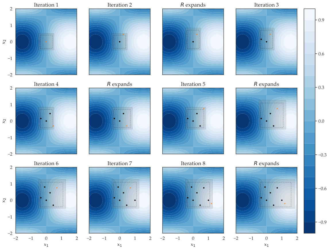
The Adaptive Region Bayesian Optimization (ARBO) [16] is a modified version of Bayesian Optimization (BO) that was developed at INFN-LNL and utilizes the base BO Python package v.1.4.3 from MIT [17], which uses a Matern Kernel ($\nu =2.5$) for its GP model and Upper Confidence Bound [18] (UCB, $\kappa =2.4$) as its acquisition function. An additional feature was added to BO in which the search region R is allowed to expand when the current best solution $X_{best}$ found by the algorithm lies near the boundary of the initially defined $R_{\mathrm{init}}$. The R is then updated for the next iteration of the optimization. The evolution of R under the ARBO algorithm is presented in Figure 1.

The expansion of R is applied independently to one or multiple parameters, depending on their proximity to the boundary, and is evaluated after each iteration. Global bounds, which the algorithm cannot exceed, are also imposed to ensure safe machine operation. With this new feature, only the dynamic expansion of the R is updated while the surrogate model and acquisition function of the BO remain unchanged. More detailed information regarding the algorithm is listed in

Table 1. Summary of the main parameters and default settings of the Adaptive Region Bayesian Optimization (ARBO) algorithm.

Feature	ARBO
Initial search region ($R_{\mathrm{init}}$)	$\{\mathbf{x}\in {\mathbb{R}}^n\mid x_i\in [x_{i,\mathrm{init}}-\Delta x_i,x_{i,\mathrm{init}}+\Delta x_i],i=1,\dots ,n\}$
Boundary proximity check	After each iteration (default)
Boundary proximity threshold	$X_{\mathrm{best}}$ lies within 10% of the boundary (default)
Region expansion factor	Expansion of the lower and/or upper bounds by 33% of current R (default)
Exploration vs. exploitation	Upper Confidence Bound (UCB) with $\kappa =2.4$ (default from BO)

.

The default parameters of the BO module were used in order to focus the study on the impact of the physics-informed initialization of the search region. The boundary proximity check can be adjusted depending on the difficulty and cost associated with evaluating the objective function. In this work, both the boundary proximity threshold and the region expansion factor were set to relatively small values to fully exploit the adaptive expansion mechanism, allowing the search region to grow only when necessary. The selection of expansion parameters introduces a trade-off: overly restrictive values limit exploration and may result in slow convergence, whereas excessively large values increase the search space and can delay convergence, especially in high-dimensional problems. The intended use of the algorithm assumes the availability of a good initial solution, typically obtained from high-fidelity physics simulations or nominal accelerator configurations, from which further optimization is performed. Consequently, the method is not designed for global optimization, but rather for efficiently refining solutions and converging to a local optimum within a reduced computational time.

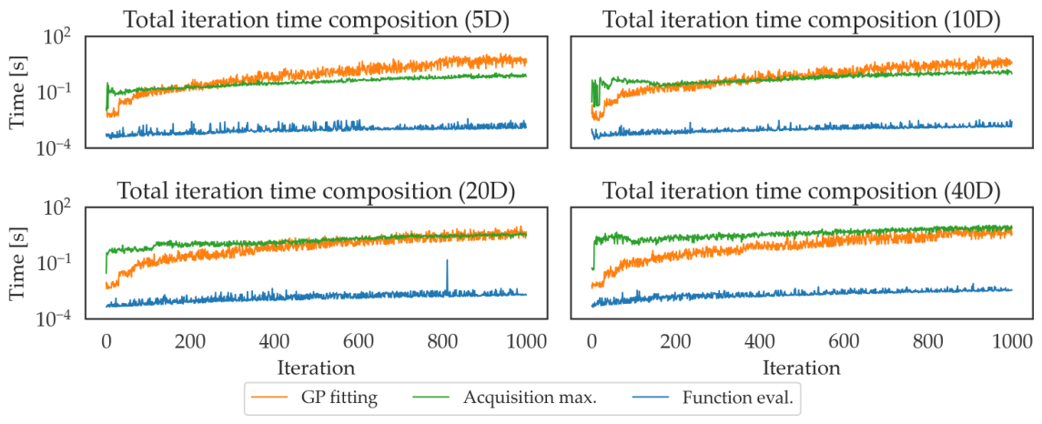
The ARBO algorithm was evaluated on the Ackley function, which is also used to benchmark TuRBO [14], across increasing input dimensions d$ϵ${$5,10,20,40$} with a fixed number of iterations $n=1000$. This function has a global search domain of [−5, 10]^d. The runtime per iteration was decomposed into three components: GP model fitting, acquisition function maximization, and objective function evaluation, as shown in Figure 2.

The objective function evaluation time (on the order of milliseconds) is negligible compared to the other components, although it shows a mild increase with both the number of samples and dimensionality. In accelerator applications, such as beam transport with particle tracking (offline) or real-time control of accelerator components (online), this cost is expected to become dominant. The GP model fitting time increases with the number of samples ($n_{1–1000}$: $8.30\pm 1.70$ ms to $3.87\pm 0.55$ s) and is independent of the input dimensionality as mentioned in [6].

In contrast, the acquisition function maximization depends on both n and d, as it involves solving a nested optimization problem. Each evaluation of the acquisition function requires computing GP posterior quantities, which involves kernel evaluations between the candidate point and all observed samples, scaling approximately as $O(n·d)$. These evaluations are performed repeatedly during the L-BFGS-B [19] optimization process, whose per-iteration cost also increases with dimensionality. Furthermore, the acquisition landscape becomes more complex in higher dimensions, leading to more expensive optimization. As a result, acquisition maximization dominates the overall iteration time with averages ranging from $0.39\pm 0.21$ s at $d=5$ to $4.37\pm 2.24$ s at $d=40$.

2.2. ARBO Parameters

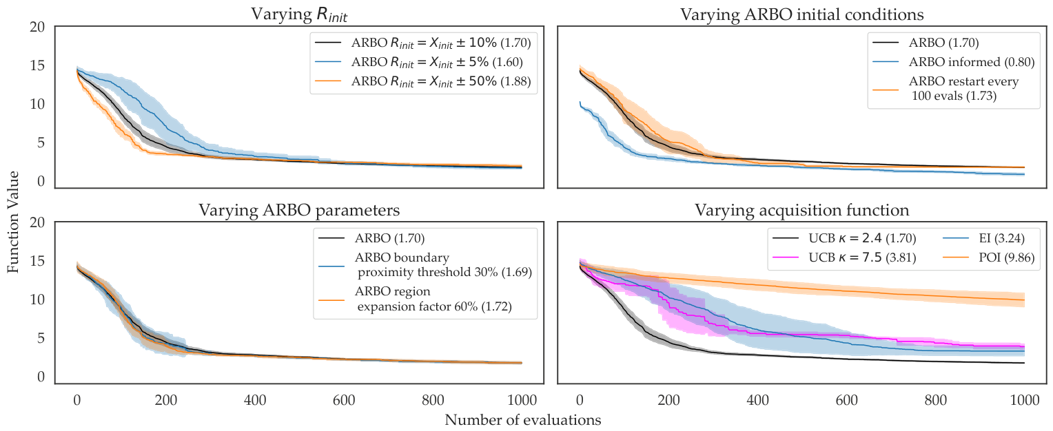
A study varying the $R_{\mathrm{init}}$, boundary proximity threshold, region expansion factor, informed starting point, and acquisition functions of the ARBO algorithm was conducted on the 40D Ackley function. Since the dimensionality of the problem cannot be easily reduced without decomposing it into lower-dimensional subproblems, an alternative strategy was investigated: restarting the optimization procedure before the computational cost becomes prohibitive due to the increasing number of observations (e.g., around $n=100$ where the total iteration time is still less than 1 s in 20D and 2 s in 40D). The results of this study are presented in Figure 3.

In this study, $R_{\mathrm{init}}$ is defined as a fraction of the global search space, centered around a randomly selected initial point. The results indicate that overly restricting $R_{\mathrm{init}}$ slows down convergence, whereas increasing $R_{\mathrm{init}}$ beyond a moderate size does not significantly improve performance. However, this behavior may not fully reflect the intended application (accelerator tuning) where different control parameters (e.g., magnetic elements or RF cavities) have varying levels of influence on the objective function. In such cases, allowing unrestricted exploration may lead to undesirable evaluations that could negatively affect the system.

An increase in both the boundary proximity threshold and in the region expansion factor had minimal impact on performance, similarly to the case of larger $R_{\mathrm{init}}$ values. Providing a more informed initial solution consistently led to faster convergence and improved final performance. Introducing periodic restarts every 100 iterations resulted in solution quality comparable to standard ARBO, while significantly reducing overall runtime. This is because the computational cost does not grow as steeply with the number of observations, although more total function evaluations are required to achieve similar performance.

With the varying acquisition functions, the performance can be ranked with UCB ($\kappa =2.4$) outperforming both UCB ($\kappa =7.5$) and Expected Improvement (EI) [20], and Probability of Improvement (POI) [21] performing worst, which can be explained by the interaction between the acquisition function and ARBO’s region-based search. A moderate $\kappa$ value in UCB provides a balanced weighting between the predicted mean and uncertainty, ensuring that uncertain regions, such as those near the boundaries, which may have moderate uncertainty but high posterior mean, are sampled efficiently without being dominated by regions of high uncertainty. In contrast, EI in high-dimensional settings can have negligible probability of improvement in large portions of the domain, causing the acquisition function to become nearly flat in those regions making it difficult to optimize [6,22] and limiting exploration of uncertain but potentially informative areas. POI, being strongly exploitative [23,24], fails to adequately explore region boundaries, leading to slower convergence and poorer overall performance.

2.3. Comparison of ARBO with Vanilla BO and TuRBO

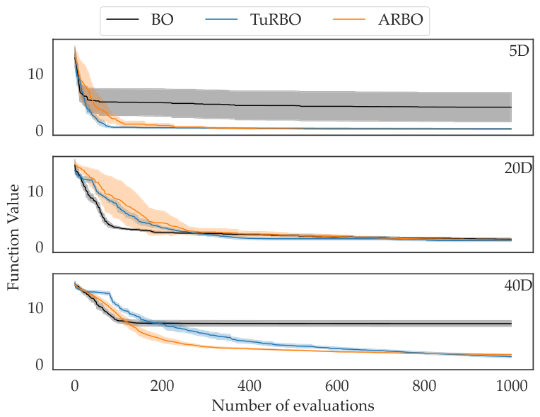
To compare the ARBO algorithm against established optimizers, namely vanilla BO and TuRBO, their performance in optimizing the Ackley function in 5D, 20D, and 40D was evaluated and the results are presented in Figure 4. The TuRBO implementation used is from [14] (v0.0.1), specifically the TuRBO-1 variant with default hyperparameter settings. Both BO and TuRBO were provided with the global search bounds, while ARBO was initialized with a local region defined as $R_{\mathrm{init}}=X_{\mathrm{init}}\pm 10\%$, corresponding to a search space covering 20% of the global search domain and was centered around a randomly selected initial setpoint.

In the 5D case, TuRBO and ARBO outperformed vanilla BO, which in several instances prematurely converged to suboptimal regions, leading to early stagnation and a larger confidence interval. In 20D, BO exhibited faster initial convergence than TuRBO and ARBO; however, all methods achieved comparable final performance. In contrast, BO performance degraded significantly in the 40D case due to the increased dimensionality and failed to reach the function values obtained by ARBO and TuRBO. Both ARBO and TuRBO converged to similar values in this setting, with ARBO showing faster convergence.

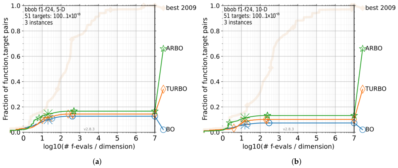
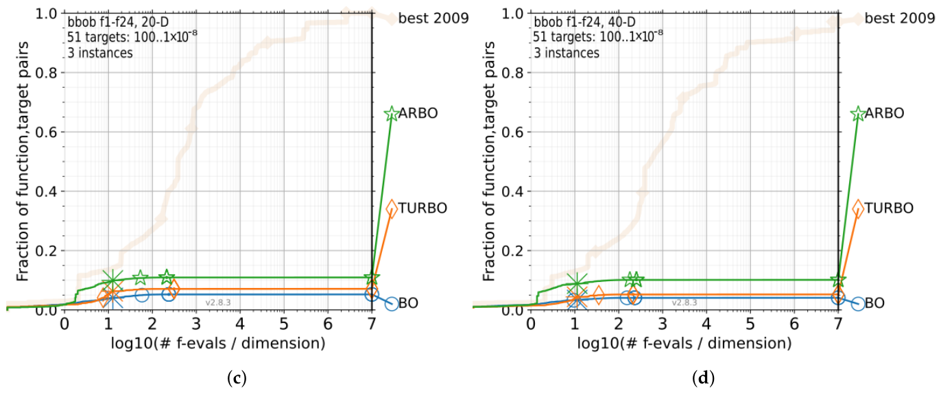
In addition, ARBO was benchmarked against BO and TuRBO-1 on the Black-Box Optimization Benchmarking (BBOB) suite from the COCO platform [25,26,27]. The results, evaluated using ECDF performance profiles across multiple dimensions (5–40D), confirm trends consistent with the Ackley experiments, with ARBO showing competitive or improved performance in higher-dimensional settings. A detailed description of the benchmark setup and results are provided in Figure A1 of Appendix C.

The main difference between ARBO and TuRBO lies in their adaptive region mechanisms. In ARBO, the initial region $R_{\mathrm{init}}$ can vary across parameters, allowing the search space to be tailored individually. This is particularly advantageous in applications such as accelerator tuning, where different parameters influence the objective function to varying degrees. In contrast to TuRBO, the adaptive expansion and contraction of the trust region based on successive successes or failures is not included in the present implementation. Instead, ARBO focuses on flexible initialization and region shaping, while the incorporation of dynamic resizing strategies during optimization remains a subject for future work.

Furthermore, the expansion of the search region in ARBO is not uniform: it is applied selectively to specific parameters that trigger the expansion criteria. In contrast, TuRBO expands or contracts the trust region uniformly across all parameters, based on the success or failure of consecutive optimization iterations. Comparisons of BO, ARBO and TuRBO applied in an accelerator setting are presented in the next section for the ANTHEM MEBT line offline optimization as well as in [16], where the methods were applied for tuning the PIAVE-ALPI accelerator at INFN-LNL.

2.4. General Methodology

To simplify the application of the algorithm to different accelerator facilities, a general workflow was developed which involves the following steps:

1.

Identify the part of the accelerator that needs to be optimized;

2.

Develop an objective function specific to the optimization problem;

3.

Determine a reasonable size for the initial search region $R_{\mathrm{init}}$;

4.

Integrate and apply the algorithm within the beam transport simulator or the accelerator control system.

2.5. EPICS Implementation to Online Accelerator Systems

The PIAVE–ALPI control system is based on Experimental Physics and Industrial Control System (EPICS) [28] and is distributed across several tens of Input/Output Controllers (IOCs), managing several thousand Process Variables (PVs) associated with magnets (quadrupoles, dipoles, steerers), RF cavities, and diagnostic instrumentation (Faraday cups, NMR probes, gauss meters). For each optimization session, ARBO operates on a selected subset of PVs, defined by the components involved.

Integration with the EPICS environment was implemented through an external Python application interfacing with PVs via the Channel Access (CA) protocol. For the ESS case, the same framework was adapted to the local computing infrastructure and control architecture, while preserving only the essential functionality required for reading and writing the relevant PVs.

At each iteration, the interaction mechanism with the accelerator follows these steps:

1.

The new setpoints computed by the algorithm are written to the control PVs via caput operations. The number of PVs written at each evaluation corresponds to the dimensionality of the optimization search space.

2.

A fixed settling time, empirically determined on the basis of preliminary measurements of the beam behaviour, is awaited to ensure system stabilization before reading the objective function. This parameter represents a potential margin for further improvement of the algorithm’s performance.

3.

The relevant beam diagnostics are read via caget and processed as described above to obtain the objective function value.

To ensure accelerator safety, software boundaries on the setpoint search space were defined and maintained throughout all optimization sessions, in addition to the hardware limits already present at the EPICS level.

2.6. Offline Optimization of the ANTHEM MEBT Line

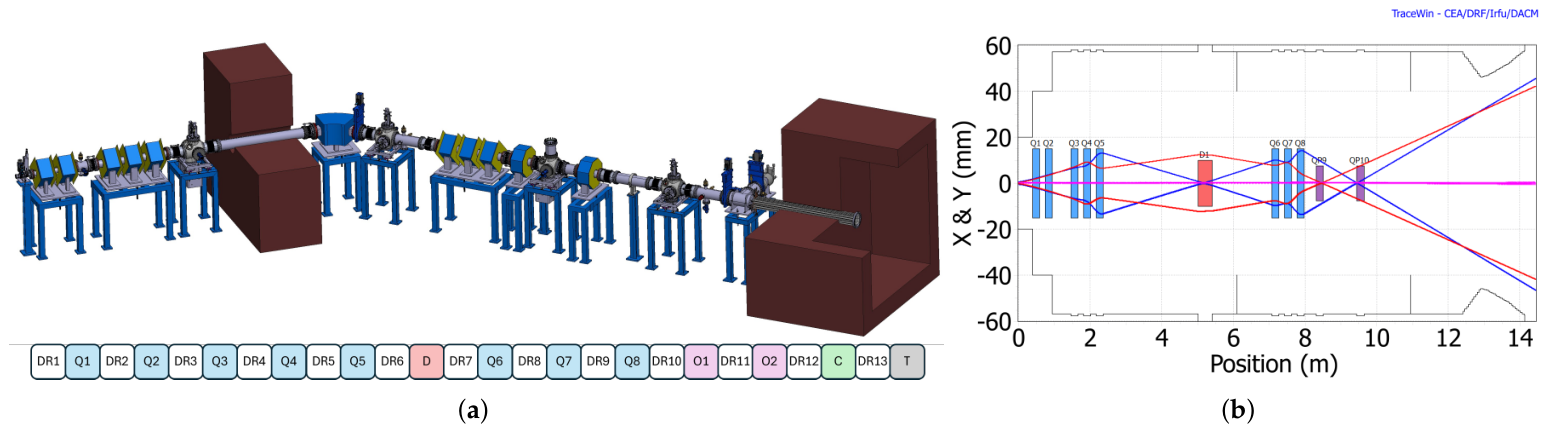
The ANTHEM research project will construct a BNCT facility in Caserta, Italy, which will utilize accelerator-based neutron beam production. A 30 mA proton beam will be accelerated to 5 MeV by the TRASCO Radio-Frequency Quadrupole (RFQ), transported through the Medium Energy Beam Transport (MEBT) line, and directed onto a beryllium target to provide the neutron flux required for treatment [29]. The optimization problem addressed in this work concerns the determination of optimal magnet settings in the MEBT, which are critical for beam transport and shaping at the target location. The key challenge is to exploit the nonlinear effects arising from the high-intensity beam and the octupole magnets to shape the beam and deliver approximately 1 kW·cm⁻² of beam power to the 120 mm×120 mm target while maintaining high beam transmission. The design of the MEBT line consists of one dipole magnet, eight quadrupole magnets, and two octupole magnets and is illustrated in Figure 5. The lengths and starting edges of each component of the MEBT are detailed in

Table A2. Magnetic element dimensions and their starting edges with respect to the start of the ANTHEM MEBT line used in the beam uniformity and transport optimizations.

Element	Length [m]	Edge [m]	Element Type
DR1	0.40	0.00	Drift
Q1	0.20	0.40	Quadrupole
DR2	0.15	0.60	Drift
Q2	0.20	0.75	Quadrupole
DR3	0.50	0.95	Drift
Q3	0.20	1.45	Quadrupole
DR4	0.15	1.65	Drift
Q4	0.20	1.80	Quadrupole
DR5	0.15	2.00	Drift
Q5	0.20	2.15	Quadrupole
DR6	2.67	2.35	Drift
D1	0.39	5.02	Dipole
DR7	1.66	5.42	Drift
Q6	0.20	7.08	Quadrupole
DR8	0.15	7.28	Drift
Q7	0.20	7.43	Quadrupole
DR9	0.50	7.63	Drift
Q8	0.20	7.78	Quadrupole
DR10	0.34	7.98	Drift
O1	0.20	8.32	Octupole
DR11	0.94	8.52	Drift
O1	0.20	9.46	Octupole
DR12	3.22	9.66	Drift
C	1.27	12.88	Collimator
DR13	0.3	14.15	Drift
T	-	14.45	Target

of Appendix A. The realistic input beam used in the beam transport simulations was obtained from a TRASCO RFQ beam dynamics simulation performed with the TOUTATIS particle-in-cell RFQ code [30], as distributed within the TraceWin framework [31], corresponding to the installation available in May 2023. The code solves the Poisson equation for a continuous beam loaded into the specified vane geometry.

Prior to the beam uniformity optimization, the beamline was first optimized to transport the beam through the MEBT without losses, with beam waists located at the positions of the octupole magnets while these elements were deactivated. This approach, known as tail-folding, was adopted to decouple the nonlinear effects of the octupoles from the beam distribution [32,33,34]. This initial optimization was performed using TraceWin v.2.23, a beam dynamics simulation code that employs a particle-in-cell (PIC) method to model beam transport and includes a built-in numerical optimizer based on the simplex algorithm [31]. Once nominal magnet settings were obtained, the last three quadrupoles and the two octupoles were optimized using vanilla BO, TuRBO, and the ARBO algorithm. The search domains for vanilla BO and TuRBO were defined as $R_k=k_{i,\mathrm{init}}\pm 0.5$ T·m⁻¹ for the quadrupoles and $R_o=o_{i,\mathrm{init}}\pm 500$ T·m⁻³, where $k_{i,\mathrm{init}}$ and $o_{i,\mathrm{init}}$ denote the nominal values. In contrast, the initial search region for ARBO was set to $R_{k,\mathrm{init}}=k_{i,\mathrm{init}}\pm \{0.05,0.1,0.5\}$ T·m⁻¹ and $R_{o,\mathrm{init}}=o_{i,\mathrm{init}}\pm \{50,100,500\}$ T·m⁻³. The latter offsets correspond to 5%, 10%, and 50% of the BO/TuRBO search domain. The smaller bounds were chosen to explore the vicinity of the nominal solution while limiting large deviations in the beam dynamics, whereas the larger bounds enable direct comparison with BO and TuRBO and illustrate the sensitivity to the choice of the initial search region $R_{\mathrm{init}}$.

The objective function was designed to balance beam uniformity u and transmission t, with the latter constrained to remain above 85% in order to ensure sufficient neutron production yield. The definitions of the beam uniformity, beam transmission, and the objective function are given in Equation (1):

$$\begin{array}{cc}\hfill u& ={\displaystyle \frac{{\rho }_{max}-{\rho }_{min}}{{\rho }_{max}+{\rho }_{min}}}\hfill \\ \hfill t& ={\displaystyle \frac{N_{\mathrm{out}}}{N_{\mathrm{in}}}}\hfill \\ \hfill \mathbf{max}f(u,t)& ={\displaystyle \frac{w_{t}t+w_{u,120}[(1-u_{x,120})+(1-u_{y,120})]+w_{u,110}[(1-u_{x,110})+(1-u_{y,110})]}{w_t+2w_{u,120}+2w_{u,110}}}\hfill \end{array}$$

(1)

Here, ${\rho }_{min}$ and ${\rho }_{max}$ denote the minimum and maximum particle densities in the beam projection, while $N_{\mathrm{in}}$ and $N_{\mathrm{out}}$ represent the number of particles at the entrance of the MEBT and at the target position, respectively. The parameters $w_t$, $w_{u,120}$, and $w_{u,110}$ are weighting factors for beam transmission and uniformity, evaluated over beam regions of 120 mm [−60, 60] mm and 110 mm [−55, 55] mm, respectively (see

Table A4. Facility−specific parameters for the ARBO algorithm applied to the different case studies.

Parameter	ANTHEM MEBT	INFN-LNL TAP	ESS-NCL
Optimized parameters $x_i$ ($i=1,\dots ,n$)	$k_i:n=3$ $o_i:n=2$	$I_{\mathrm{d},\mathrm{i}}^{\mathrm{norm}}:n=16$ $I_{k,i}^{\mathrm{ave}}:n=11$ $I_{k,i}^{\mathrm{unb}}:n=10$ ${\varphi }_i:n=40$	$d_i:n=52$ $k_i:n=4$ $V_{\mathrm{acc},i}:n=3$ ${\varphi }_i:n=3$
Initial search bounds $\Delta x_i$ ($R_{\mathrm{init}}=[x_{i,\mathrm{init}}\pm \Delta x_i]$)	$\Delta k_i:\pm 0.05,0.1,0.5$ T·m−1 $\Delta o_i:\pm 50,100,500$ T·m−3	$\Delta I_{\mathrm{d},\mathrm{i}}^{\mathrm{norm}}:\pm 2$ % $\Delta I_{k,i}^{\mathrm{ave}}:\pm 0.5$ % ($\pm 0.05$–$0.24$ T·m−1) * $\Delta I_{k,i}^{\mathrm{unb}}:\pm 0.003$ $\Delta {\varphi }_i:\pm 2$ deg	$\Delta d_i:\pm 0.36$ A ($\pm 2$ mT) $\Delta k_i:\pm 0.6$ A ($\pm 0.1$ T·m−1) $\Delta V_{\mathrm{acc},i}:\pm 1$ V $\Delta {\varphi }_i:\pm 2$ deg
Number of diagnostics/observables used in the objective functions	$u:4,t:1$	$I:1$	$I:2,c:50,s:291$
Objective weighting factors w	$w_t=1.5$, $w_{u,120}=0.25$, $w_{u,110}=0.75$	–	$f_t:w_I=100,w_c=1$
			$f_l:w_I=5000,w_s=1$

* Depends on the magnet calibrations.

in Appendix B for the values used).

The selection of appropriate weighting factors is critical for balancing optimization performance and was determined through a preliminary hyperparameter optimization. Transmission was assigned a higher weight than uniformity, as beam losses can significantly impact both the target and upstream components if not properly controlled.

Furthermore, enforcing a sharp, square beam profile can lead to strong edge effects in the density distribution, which may bias the uniformity metric. To mitigate this, the uniformity was evaluated over two regions: a wider interval [−60, 60] mm and a narrower core region [−55, 55] mm, with the latter assigned a higher weight.

TraceWin, which was used solely for beam transport simulations, was coupled with the optimization algorithms, which acted as an external optimizer to explore the parameter space and select the next set of parameters to be evaluated. A summary of the key parameters used for the TraceWin particle tracking simulations are listed in

Table A1. Summary of the key parameters for the TraceWin particle tracking simulation of the ANTHEM MEBT line.

Variable	Value	Description
Particle	Proton	Particle type used for the simulation.
Number of particles	207,611	Number of particles used for the simulation.
Energy	5 MeV	Energy of the particles used for the simulation.
Beam current	31.12 mA	Beam current used for the simulation.
${ϵ}_{x{x}^{\prime }}$	0.22 $\pi$.mm.mrad	X-X’ normalized RMS emittance of the input beam.
${ϵ}_{y{y}^{\prime }}$	0.25 $\pi$.mm.mrad	Y-Y’ normalized RMS emittance of the input beam.
${ϵ}_{\varphi w}$	1.78 $\pi$.deg.MeV	Longitudinal RMS emittance of the input beam.
Space-charge routine	PICNIC(3D)	Space-charge routine used for the simulation.
Mesh (x-y, z)	6, 6	3D mesh for the Particle In Cells integration.
Calculation step	${\displaystyle \frac{50}{\beta \lambda }}$	The number of calculation step for particle tracking.
Space-charge step	${\displaystyle \frac{25}{\beta \lambda }}$	The number of space-charge kicks for particle tracking.

of Appendix A. The beam projection and beam transmission at the target were extracted and computed from the TraceWin output files.

2.7. Online Optimization of the INFN-LNL TAP Facility

The INFN-LNL TAP accelerator complex comprises the ALPI superconducting linear accelerator, which consists of 20 cryostats (CRs), each housing four quarter-wave cavities. These cavities were originally designed to operate at an accelerating gradient of 3 MV·m⁻¹ with a 10 mm bore aperture and require independent tuning depending on the ion species. The lattice design of ALPI employs a triplet focusing structure for every two cryostats in order to maximize space efficiency. Over the years, advancements in superconducting technology have nearly doubled the achievable accelerating fields of the cavities; however, this improvement has resulted in reduced transmission efficiency [35].

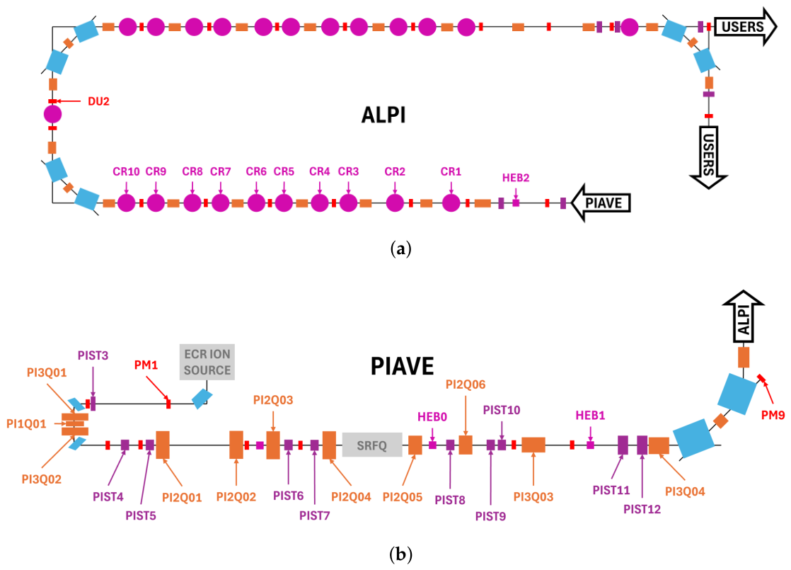
The TAP complex features two injectors: the electrostatic TANDEM accelerator, which accelerates light ions, and the PIAVE superconducting RFQ, which accelerates heavier ions to an output energy of 587.5 keV·u⁻¹. Both injectors suffer from low transmission to ALPI due to the aggressive focusing of the ALPI lattice, which makes the system highly sensitive to beam misalignments. The design transmission efficiency of the ALPI–PIAVE configuration is approximately 65% (PIAVE: 70% maximum, ALPI: 93% maximum [35]); however, the actual operational transmission is typically around 20% (PIAVE: 55% on average, ALPI: 35% on average [35]). These operational values are significantly lower than the theoretical limits, as machine setup is complex and frequent instabilities shift the optimal working point, requiring re-optimization every few hours. Further details regarding the beam dynamics limitations of ALPI are discussed in [35]. The layout of the ALPI-PIAVE facility is presented in Figure 6.

From 19–27 June 2024, a series of ML-based beam transport optimization tests were performed at the ALPI-PIAVE with a ${}^{129}\mathrm{Xe}^{\text{25+}}$ beam. More information regarding the beam parameters used in the tests is provided in

Table A3. Summary of the key parameters for the ML-based beam optimization at INFN-LNL TAP facility and ESS.

Variable	Value	Description
INFN-LNL TAP facility
Beam	${}^{129}\mathrm{Xe}^{\text{25+}}$	Type of beam optimized.
Energy	587.5 keV·u−1 (end of PIAVE) 4.9 MeV·u−1 (at FC DU2)	Energy of the beam during optimization.
Beam current	∼900 nA	Beam current from ion source during optimization.
ESS
Beam	Proton	Type of beam optimized.
Energy	90 MeV (end of DTL) 0.8 GeV (at Beam dump, cavities until HBL05 active)	Energy of the beam during optimization.
Beam current	∼5 mA	Beam current from ion source during optimization.
Pulse length	5 $\mathrm{\mu }$s	Pulse length of the beam during optimization.
Repetition rate	1 Hz	Repetition rate of the beam pulse during optimization.

of Appendix A. Due to the lack of diagnostics along the beamline, the beam current measured with Faraday Cups (FCs) was the sole performance indicator available to the optimization algorithm and therefore served as the objective function to be maximized (Equation (2)).

$$\mathbf{max}f\left(I\right)=I_{\mathrm{FC}}$$

(2)

FC measurements were performed by waiting two seconds after the accelerator components reached their setpoints, after which five readings were taken at 0.5 s intervals. The maximum value among the five readings was then returned to the algorithm, provided it exceeded the a noise threshold of 0.5 nA (empirically determined from baseline FC fluctuations).

Transverse and longitudinal optics were optimized separately to determine suitable initial search regions, $R_{\mathrm{init}}$, for each parameter. This was achieved by performing runs of approximately 100 iterations with progressively increasing $R_{\mathrm{init}}$ and selecting the value that provided the best performance for subsequent optimizations. The tested $R_{\mathrm{init}}$ values were relatively small (<10% of the maximum applied current for magnets and <10° for cavity phases), as the initial settings were derived from beam transport simulations or from magnet scaling based on the beam $A/q$.

The transverse optimization included the applied quadrupole currents ($I_{\mathrm{Q},i}^{\mathrm{ave}}$, $I_{\mathrm{Q},i}^{\mathrm{unb}}$) and steerer currents ($I_{\mathrm{d},i}^{\mathrm{norm}}$), while the longitudinal optimization involved the cavity and buncher phases (${\varphi }_i$).

2.8. Online Optimization of the ESS-NCL

In contrast, the European Spallation Source (ESS) is a high-intensity proton linear accelerator designed for neutron production via spallation. It is divided into two main sections: the normal conducting linac (NCL) and the superconducting linac (SCL). The accelerator is designed to operate at a duty cycle of 4% (2.86 ms beam pulses at 14 Hz repetition rate) and to accelerate a proton beam with a peak current of 62.5 mA to an energy of 2 GeV. The operational frequencies are 352.21 MHz for the NCL and spoke cavities, and 704.42 MHz for the elliptical cavities [36].

This study focused on the optimization of the NCL section, specifically the matching between the MEBT line and the Drift Tube Linac (DTL), which is critical for proper beam injection into the superconducting linac. Controlling beam losses along the beamline was the primary challenge, as even low-duty-cycle losses can damage the machine. Beam current alone is insufficient to achieve the desired matching because the ESS design features a large acceptance. Therefore, additional diagnostic metrics, including beam trajectories measured by beam position monitors (BPMs) and beam loss signals from beam loss monitors (BLMs), were incorporated into the optimization. The layout of the ESS linac is shown in Figure 7.

From 10–12 June 2025, transverse and longitudinal optics were optimized separately using different combinations of diagnostic metrics to construct the objective function. Details on the beam parameters used in these tests are provided in Table A3 of Appendix A. The transverse optimizations included MEBT quadrupoles ($k_i$) and steerers ($d_i$), as well as DTL steerers, while monitoring beam trajectories and beam current up to the exit of DTL5, where the beam was dumped. To rigorously test the algorithm, the beam was intentionally misaligned at the entrance of the MEBT, resulting in initial beam losses exceeding 20%.

For the longitudinal optimization, the beam was accelerated to the dump with both the NCL and SCL active, reaching a proton energy above 800 MeV [36]. The phases (${\varphi }_i$) and fields ($V_{\mathrm{acc},i}$) of the MEBT bunchers were optimized to improve matching between the MEBT and DTL, while monitoring beam transmission to the dump and BLM signals along the SCL section.

The initial search region, $R_{\mathrm{init}}$, for each parameter was determined from pre-experimental simulations through short runs exploring different values of $R_{\mathrm{init}}$. Starting from the nominal design settings of the ESS linac, the tested $R_{\mathrm{init}}$ values were kept relatively small to avoid introducing large perturbations that could lead to uncontrolled beam losses. The objective functions for the transverse, $f_t$, and longitudinal, $f_l$, optimizations are defined as follows:

$$\begin{array}{cc}\hfill \mathbf{max}{f}_t(I,c)& ={\displaystyle \frac{w_I\left(-\frac{|I_{\mathrm{RFQ},\mathrm{exit}}-I_{\mathrm{DTL}5,\mathrm{exit}}|}{I_{\mathrm{RFQ},\mathrm{exit}}}\right)+w_c{\sum }_{i=1}^n(-|c_{x,i}\left|\right)+w_c{\sum }_{i=1}^m(-|c_{y,i}\left|\right)}{w_I+w_{c}n+w_{c}m}}\hfill \\ \hfill \mathbf{max}{f}_l(I,s)& ={\displaystyle \frac{w_I\left(\frac{I_{\mathrm{Dump}}}{I_{\mathrm{RFQ},\mathrm{exit}}}\right)+w_s\left(\frac{1}{n}{\sum }_{i=1}^n{s}_i\right)}{w_I+w_s}}.\hfill \end{array}$$

(3)

Here, $I_{\mathrm{RFQ},\mathrm{exit}}$, $I_{\mathrm{DTL}5,\mathrm{exit}}$, and $I_{\mathrm{Dump}}$ denote the beam currents measured at the RFQ exit, the DTL5 exit, and the beam dump, respectively. The quantities $c_{x,i}$ and $c_{y,i}$ represent the horizontal and vertical beam trajectory deviations measured by the beam position monitors, while $s_i$ denotes the beam loss signal measured by the beam loss monitors. The parameters $w_I$, $w_c$, and $w_s$ are weighting factors that balance the relative importance of beam transmission, trajectory control, and beam loss minimization.

The ratio between $w_I$ and $w_c$ is intentionally skewed, as the primary goal was to avoid beam losses along the beamline; thus, the optimizer is first driven to maximize transmission before fine-tuning the trajectory. This effect was further emphasized in the longitudinal optimization, where the beam was transported up to the dump with the SCL cavities activated, requiring more conservative weighting to ensure transmission preservation.

Five diagnostic measurements (BPMs, BCMs, and BLMs, depending on the test) were acquired every second following a two-second settling time after reaching the accelerator component setpoints. In contrast to the PIAVE–ALPI case, the average of the readings was computed and returned to the optimizer instead of the maximum value. The BPMs have a position accuracy of $\pm 400\mathrm{\mu }$m at 6.3 mA and a 5 $\mathrm{\mu }$s pulse length [37], while the BCMs have an accuracy of approximately 0.1 mA with a noise level below 50 $\mathrm{\mu }$A [38]. During the tests, the BLMs were not yet calibrated; therefore, their signals are reported in relative units. A noise threshold of 0.5 a.u. (arbitrary units), determined empirically, was applied to improve discrimination between noise and true loss events, with values below this threshold set to zero in the objective function evaluation. Further details regarding the number of parameters optimized and their initial search regions used in all three tests (ANTHEM, PIAVE-ALPI, ESS) are listed in Table A4 of Appendix B.

3. Results

3.1. Beam Uniformity Optimization in the ANTHEM MEBT Line

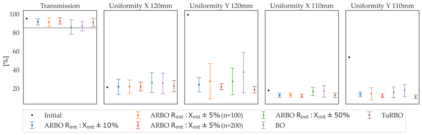
The transport and uniformity of the proton beam through the MEBT line were optimized using vanilla BO, TuRBO, and ARBO, each run 20 times with different random seeds for $n=100$ iterations (with an additional $n=200$ iterations for ARBO with $R_{\mathrm{init}}=X_{\mathrm{init}}\pm 5\%$). The beam transmission and uniformity achieved by the best solutions found by each algorithm are presented in Figure 8. The average beam transmission across all algorithms exceeds the 85% requirement; however, some runs using BO and ARBO with a larger initial search region, comparable to that used in BO and TuRBO, yielded transmission values below this threshold.

The beam uniformity over a 120 mm region improved from initial values of 21.12% and 99.18% in the horizontal and vertical planes, respectively, to mean values below 30% and 40% after optimization. The improvement was most pronounced in the vertical plane, while the horizontal plane remained at a comparable level. Within the 110 mm region, all uniformity values were below 20%, indicating a clear improvement from the initial distribution. ARBO with $R_{\mathrm{init}}=X_{\mathrm{init}}\pm 5\%$ was allowed to continue up to $n=200$ iterations and achieved better overall performance than the $R_{\mathrm{init}}=X_{\mathrm{init}}\pm 10\%$ configuration, albeit requiring more iterations. This highlights the trade-off between faster convergence and improved solution quality.

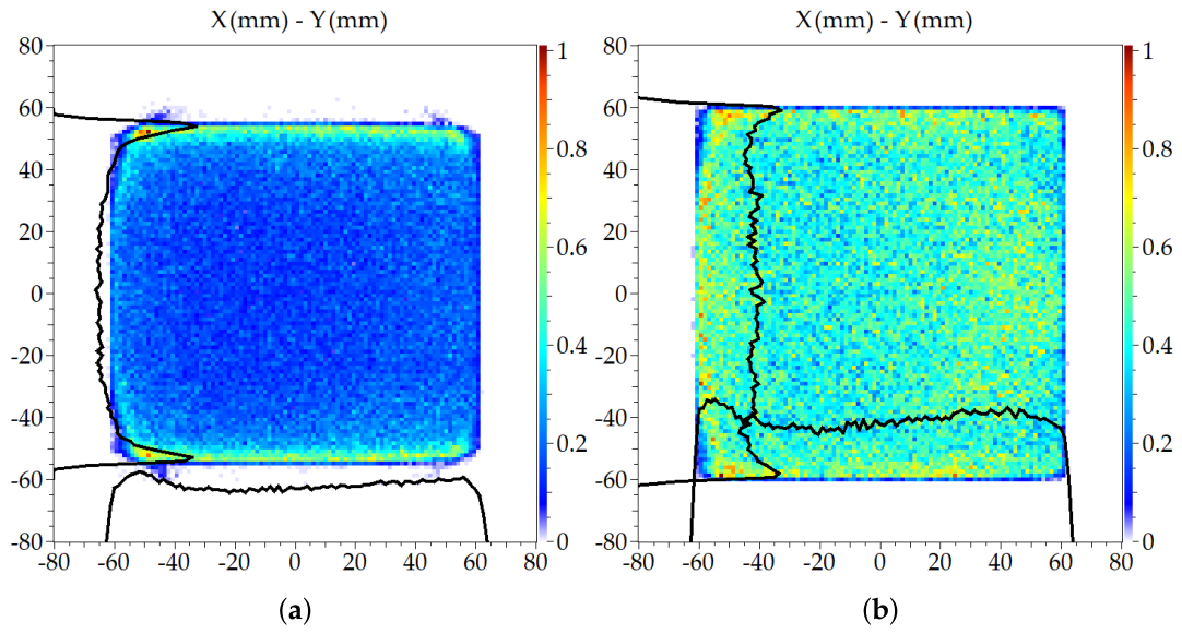
Figure 9 shows the beam distribution, together with the horizontal and vertical projections at the target position, before and after optimization (best ARBO run with $R_{\mathrm{init}}=X_{\mathrm{init}}\pm 10\%$). This run achieved beam uniformities of ±16.54% in the horizontal direction and ±17.52% in the vertical direction over a 120 mm × 120 mm beam area, while maintaining a high transmission of 92.09%.

3.2. Beam Transport Optimization of the INFN-LNL TAP Facility

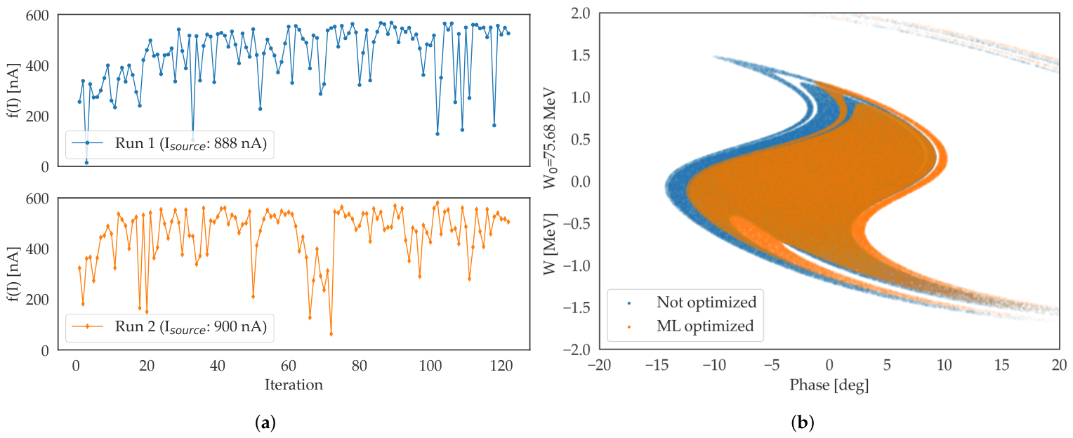
The results of the transverse and longitudinal beam transport optimizations performed at the INFN-LNL ALPI-PIAVE accelerator complex are presented in Figure 10. The extracted source current measured at Faraday Cup PM1 during the week-long experiment was $861\pm 42$ nA and could only be measured before and after each optimization run, as the Faraday cup intercepts the full beam.

By applying ARBO to optimize all 37 transverse parameters (quadrupoles and steerers) of PIAVE, the beam current through PIAVE increased from 254 nA to 567 nA (Figure 10a, Run 1), corresponding to an improvement in beam transmission from approximately 33.7% to 64.6% at the exit of PIAVE (Faraday cup PM9). This improvement was achieved under stable source conditions, with the source current varying only from 882 nA to 888 nA. The result was obtained in 120 iterations, corresponding to less than 18 min of optimization time, and represents a substantial improvement over typical operational transmission, approaching the expected theoretical performance. A second optimization run (Figure 10a, Run 2) yielded consistent results, with beam transmission increasing from 35.8% to 64.5%.

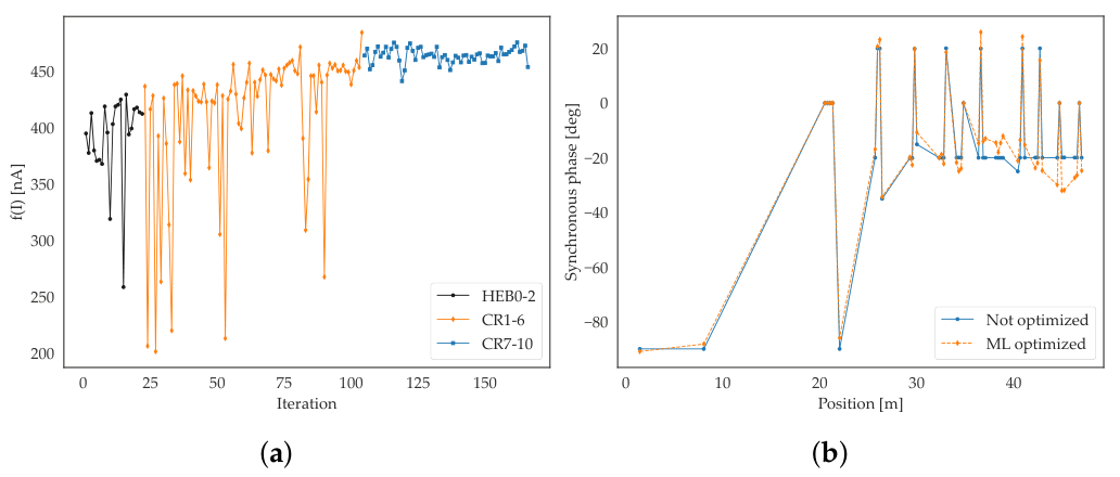
The longitudinal optics optimization was carried out through sequential runs, each focusing on a specific subset of elements. The optimized parameters, in the order of the runs, were: (1) HEB0-2 bunchers (3 parameters), (2) cryostats 1–6 (23 parameters), and (3) cryostats 7–10 (14 parameters). Before the longitudinal optics optimization, transverse optimization (both scaled settings and ARBO-based optics optimizations) for ALPI during gradual beam acceleration and re-optimization of both PIAVE and ALPI optics after CR10 beam acceleration were already performed. This sequential optimization increased the beam current measured at Faraday cup DU2, located at the midpoint of ALPI, from 394 nA to 475 nA, indicating an increase in beam transmission from approximately 44.2% (PIAVE ∼64%, ALPI ∼69%) to 52.6% (PIAVE ∼64%, ALPI ∼82%) through the PIAVE-mid ALPI section with the source current relatively stable (884 nA to 896 nA). This result was obtained after a total of 160 iterations (Run 1: 20 iterations, Run 2: 80 iterations, Run 3: 60 iterations). Figure A2 of Appendix C shows the evolution of the objective function for longitudinal optimization as a function of the algorithm iterations, as well as the synchronous phases of the bunchers and cavities before and after the optimization.

Figure 10b illustrates the longitudinal acceptances of ALPI up to DU2 before (black) and after (red) the optimization. The acceptances were computed in TraceWin by transporting a beam with large longitudinal emittance and a high number of particles through ALPI, and then tracking the surviving particles at the DU2 back to the entrance. The optimized changes in the synchronous phases of the bunchers and cavities resulted in a distortion of the acceptance shape, enhancing its coverage in the positive phase ($+\varphi$) direction.

3.3. Beam Transport Optimization in the ESS-NCL

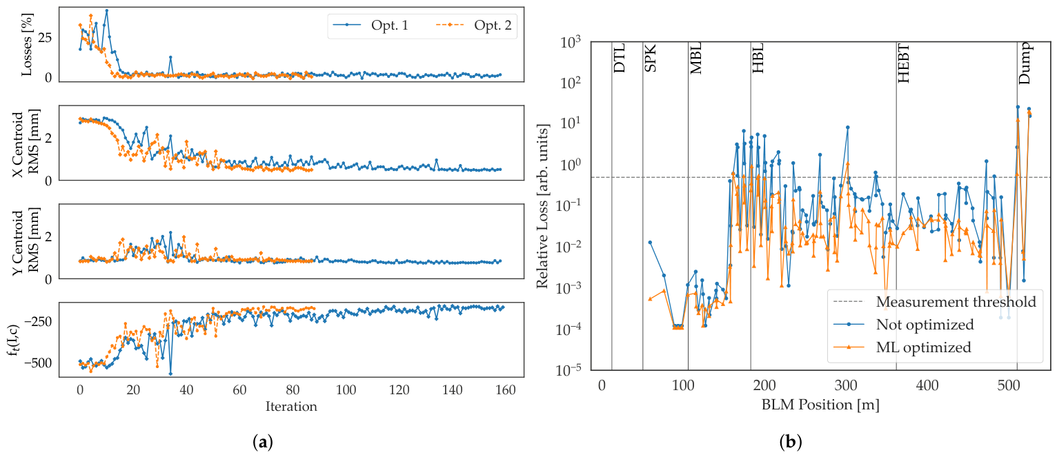
The results of the transverse and longitudinal beam transport optimizations performed at ESS are presented in Figure 11. For the transverse optics optimization of the ESS-NCL, 56 (Opt. 1: quadrupoles and steerers) and 52 (Opt. 2: steerers only) parameters were simultaneously tuned. The starting points of the two optimization runs are different since the for Opt. 1 the quadrupoles were also changed on top of the steerers. To accelerate convergence, the optimizations were divided into shorter sequential runs. Opt. 1 was performed in two runs, with a restart after 50 iterations, while Opt. 2 was carried out over four consecutive runs with restarts every 40 iterations.

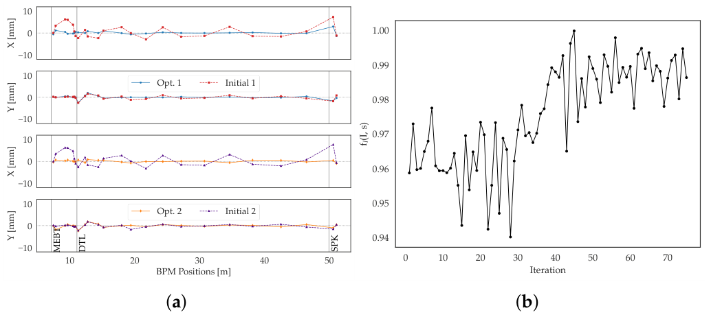
The evolution of the objective function as a function of accumulated iterations, together with the beam loss and the horizontal and vertical RMS beam centroid, is shown in Figure 11a. In Opt. 1, the optimization increased beam transmission from 67.4% to 99.4% and reduced beam losses within the first 20 iterations, requiring less than three minutes of optimization time. Subsequently, the algorithm focused on minimizing beam trajectory offsets. The horizontal and vertical beam trajectories from the MEBT to the first spoke cavities, before and after optimization, are shown in Figure A3a of Appendix C. The final optimized solution was obtained after 52 iterations, corresponding to less than ten minutes of total optimization time. A similar trend was observed for Opt. 2, where the algorithm initially prioritized transmission improvement before refining the beam trajectory.

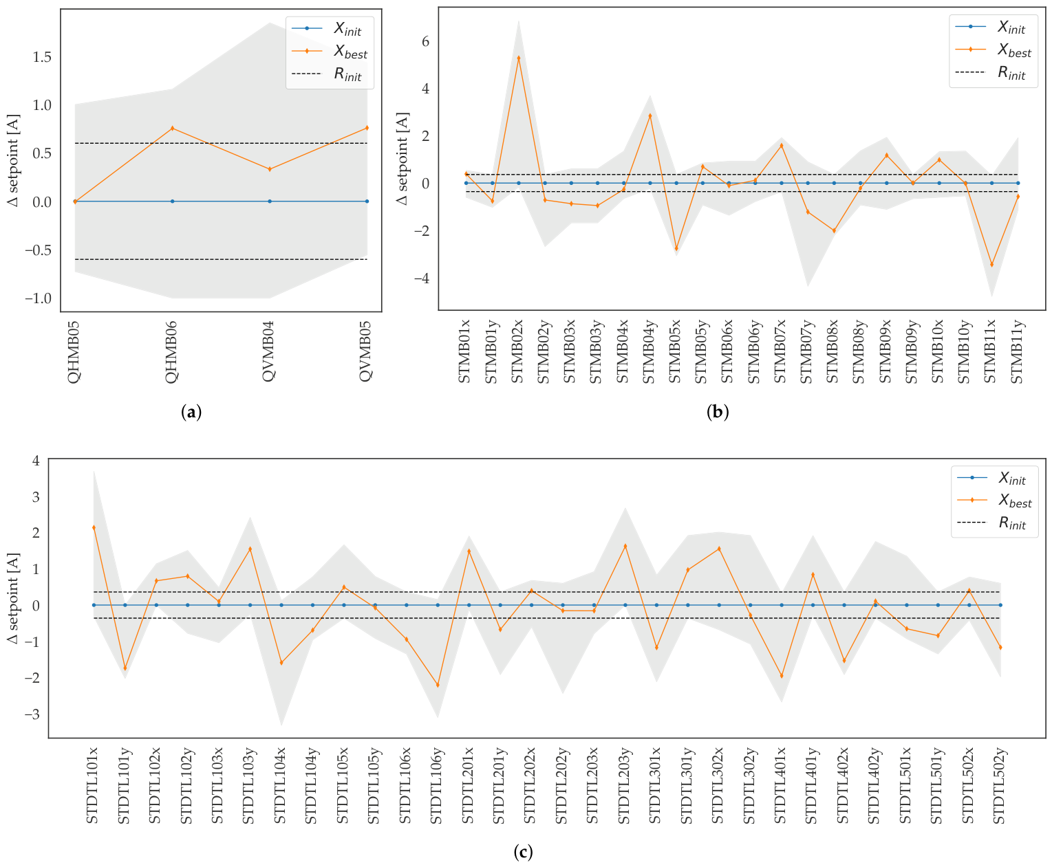
To illustrate the effectiveness of the adaptive region feature of ARBO, the parameter values explored by the algorithm during the optimization are shown in Figure A4 of Appendix C. Even with a more restrictive initial search region, as in the ESS case, the algorithm was able to explore and identify optimal solutions well beyond the initial boundaries.

The longitudinal optics optimization focused on the MEBT bunchers while monitoring beam loss monitor signals along the superconducting linac. Figure 11b shows the beam loss signals as a function of beam loss monitor position along the linac before and after optimization. Prior to optimization, significant beam losses were observed at the interface between the medium-$\beta$ linac (MBL) and the high-$\beta$ linac (HBL), which is after the frequency jump. These losses were substantially reduced following the machine learning based optimization. In addition, the overall beam transmission to the beam dump increased from 96.3% to 99.1%. A total of 75 iterations were performed, with the optimal solution reached at the 45th iteration in under ten minutes, as shown in Figure A3b of Appendix C.

4. Discussion

In this work, the ARBO algorithm was evaluated against vanilla BO and TuRBO using both benchmark test functions and experimental studies at three facilities, spanning offline and online optimization scenarios with distinct objectives. With its newly introduced features, ARBO successfully optimized the MEBT design of the ANTHEM BNCT facility in simulations, as well as beam transport in the INFN-LNL TAP facility and the European Spallation Source through online transverse and longitudinal optics optimizations. These machine learning-based approaches streamline both design and machine setup processes by efficiently sampling magnet and cavity settings, reducing the time required to achieve the desired beam characteristics.

From the benchmark function comparisons, ARBO showed performance comparable to BO and TuRBO for dimensionalities below $d<20$ while outperforming them in higher-dimensional problems. Nevertheless, further developments are needed, particularly in adaptive region management, including potential contraction strategies to avoid unnecessary sampling an early termination if a specified target is reached, and in extending the approach to parameter-specific trust regions, similar to TuRBO. Additional studies on high-dimensional systems, especially in comparison with TuRBO, are required to better assess the algorithm’s capabilities and limitations. More systematic strategies for defining $R_{\mathrm{init}}$ across accelerator components should also be explored.

For the ANTHEM MEBT optimization ($d=5$), ARBO with a physics-informed $R_{\mathrm{init}}$ achieved performance comparable to TuRBO. This highlights its potential even in low-dimensional settings, although validation on more complex configurations is still needed. An error study including beam input variations and magnet misalignments will be conducted around the optimized solution, and ARBO will be integrated into the beam tuning routine for commissioning and operation.

At the INFN-LNL TAP facility, beam transport optimization resulted in significant improvements in beam delivery and reduced machine downtime. The ARBO-based tests consistently revealed a shift in ALPI’s longitudinal acceptance, attributed to phase drifts likely caused by timing differences between PIAVE and ALPI or temperature fluctuations. These findings motivate further integration of machine learning-based algorithms into machine setup and tuning for future campaigns. A dedicated investigation is planned to identify the origin and location of these phase drifts, which could inform component upgrades or replacements.

At ESS, beam transport optimization demonstrated ARBO’s potential for broader application in high-intensity accelerator facilities. Physics-informed constraints, implemented through a restricted initial search region and a large weighting factor on beam transmission, guided the algorithm away from potentially unsafe regions. Combined with ARBO’s adaptive high-dimensional search strategy, this enabled efficient exploration while maintaining stable optimization behavior, allowing the simultaneous tuning of 56 parameters. Both transverse and longitudinal optimizations improved matching between the MEBT and DTL sections, as reflected by reduced BLM signals downstream of the frequency jump, where longitudinal acceptance is limited. Improved upstream matching further reduced losses after the frequency transition by minimizing longitudinal beam emittance and maintaining the beam within the acceptance. Comparison with simulations revealed a qualitative correlation between experimental losses at the frequency jump and phase offsets from the RFQ when varying the beam current, consistent with previous observations [39]. Future work will include a repeat of the ML-based optimization tests using calibrated BLM signals to improve the reliability of loss measurements. The methodology will then be extended to the SCL section of ESS to evaluate its performance in a higher-energy regime.

For both online case studies, improvements in data acquisition and processing, as well as more robust handling of noise from diagnostics and the system, are expected to further enhance optimization performance.

5. Conclusions

In this work, we demonstrated the applicability of a machine learning-based optimization framework (ARBO) for accelerator tuning and design across simulated and operational beamlines. The algorithm was benchmarked against vanilla Bayesian Optimization and TuRBO, and validated in three experimental facilities covering both offline design and online beam tuning scenarios.

Across all case studies, ARBO enabled efficient optimization of high-dimensional parameter spaces using a single-valued objective function, leading to consistent improvements in beam quality, transmission, and operational stability. The results highlight the importance of incorporating physics knowledge into the optimization process, particularly through the definition of the objective function and the selection of physically meaningful parameter bounds.

Future developments will focus on improving adaptive search strategies and extending the methodology to more complex high-dimensional accelerator systems, with the goal of further enhancing robustness, generalization, and automation in accelerator tuning.

References

1. Nagaitsev, S.; Huang, Z.; Power, J.; Vay, J.L.; Piot, P.; Spentzouris, L.; Rosenzweig, J.; Cai, Y.; Cousineau, S.; Conde, M.; et al. Accelerator and Beam Physics Research Goals and Opportunities. arXiv 2021, arXiv:2101.04107. [Google Scholar] [CrossRef]
2. U.S. Department of Energy, Office of Science. Accelerator and Beam Physics Roadmap 2023; U.S. Department of Energy, Office of Science: Washington, DC, USA, 2023.
3. Nelder, J.A.; Mead, R. A Simplex Method for Function Minimization. Comput. J. 1965, 7, 308–313. [Google Scholar] [CrossRef]
4. Huang, X. Robust simplex algorithm for online optimization. Phys. Rev. Accel. Beams 2018, 21, 104601. [Google Scholar] [CrossRef]
5. Huang, X.; Corbett, J.; Safranek, J.; Wu, J. An algorithm for online optimization of accelerators. Nucl. Instrum. Methods Phys. Res. Sect. A 2013, 726, 77–83. [Google Scholar] [CrossRef]
6. Roussel, R.; Edelen, A.L.; Boltz, T.; Kennedy, D.; Zhang, Z.; Ji, F.; Huang, X.; Ratner, D.; Santamaria Garcia, A.; Xu, C.; et al. Bayesian optimization algorithms for accelerator physics. Phys. Rev. Accel. Beams 2024, 27, 084801. [Google Scholar] [CrossRef]
7. Ferran Pousa, A.; Jalas, S.; Kirchen, M.; Martinez de la Ossa, A.; Thévenet, M.; Hudson, S.; Larson, J.; Huebl, A.; Vay, J.L.; Lehe, R. Bayesian optimization of laser-plasma accelerators assisted by reduced physical models. Phys. Rev. Accel. Beams 2023, 26, 084601. [Google Scholar] [CrossRef]
8. Xu, C.; Boltz, T.; Mochihashi, A.; Santamaria Garcia, A.; Schuh, M.; Müller, A.S. Bayesian optimization of the beam injection process into a storage ring. Phys. Rev. Accel. Beams 2023, 26, 034601. [Google Scholar] [CrossRef]
9. Jalas, S.; Kirchen, M.; Messner, P.; Winkler, P.; Hübner, L.; Dirkwinkel, J.; Schnepp, M.; Lehe, R.; Maier, A.R. Bayesian Optimization of a Laser-Plasma Accelerator. Phys. Rev. Lett. 2021, 126, 104801. [Google Scholar] [CrossRef] [PubMed]
10. Kaiser, J.; Xu, C.; Eichler, A.; Santamaria Garcia, A.; Stein, O.; Bründermann, E.; Kuropka, W.; Dinter, H.; Mayet, F.; Vinatier, T.; et al. Reinforcement learning-trained optimisers and Bayesian optimisation for online particle accelerator tuning. Sci. Rep. 2024, 14, 15733. [Google Scholar] [CrossRef]
11. Duris, J.; Kennedy, D.; Hanuka, A.; Shtalenkova, J.; Edelen, A.; Baxevanis, P.; Egger, A.; Cope, T.; McIntire, M.; Ermon, S.; et al. Bayesian Optimization of a Free-Electron Laser. Phys. Rev. Lett. 2020, 124, 124801. [Google Scholar] [CrossRef]
12. Shahriari, B.; Swersky, K.; Wang, Z.; Adams, R.P.; de Freitas, N. Taking the Human Out of the Loop: A Review of Bayesian Optimization. Proc. IEEE 2016, 104, 148–175. [Google Scholar] [CrossRef]
13. Rasmussen, C.E.; Nickisch, H. Gaussian Processes for Machine Learning (GPML) Toolbox. J. Mach. Learn. Res. 2010, 11, 3011–3015. [Google Scholar]
14. Eriksson, D.; Pearce, M.; Gardner, J.R.; Turner, R.; Poloczek, M. Scalable Global Optimization via Local Bayesian Optimization. In Proceedings of the Advances in Neural Information Processing Systems (NeurIPS 2019), Vancouver, BC, Canada, 8–14 December 2019. [Google Scholar] [CrossRef]
15. Liuzzo, S.M.; Agapov, I.V.; Böse, M.; Carmignani, N.; Carver, L.R.; Edelen, A.L.; Hellert, T.; Hoummi, L.; Keil, J.; Lacoste, D.; et al. Optimisation of the Touschek Lifetime in Synchrotron Light Sources Using Badger. In Proceedings of the 19th International Conference on Accelerator and Large Experimental Physics Control Systems (ICALEPCS’23), Cape Town, South Africa, 9–13 October 2023; pp. 108–115. [Google Scholar] [CrossRef]
16. Ong, Y.K.; Bellan, L.; Bortolato, D.; Montis, M.; Comunian, M.; Pisent, A.; Fagotti, E. ALPI-PIAVE performance at INFN-LNL with advanced optimization algorithms. In Proceedings of the 16th International Conference on Heavy Ion Accelerator Technology (HIAT 2025), East Lansing, MI, USA, 22–27 June 2025; pp. 211–214. [Google Scholar] [CrossRef]
17. Nogueira, F. Bayesian Optimization: Open Source Constrained Global Optimization Tool for Python, version 1.4.3; GitHub; 2014. Available online: https://github.com/bayesian-optimization/BayesianOptimization (accessed on 25 May 2026).
18. Srinivas, N.; Krause, A.; Kakade, S.M.; Seeger, M. Gaussian Process Optimization in the Bandit Setting: No Regret and Experimental Design. arXiv 2009, arXiv:0912.3995. [Google Scholar] [CrossRef]
19. Zhu, C.; Byrd, R.H.; Lu, P.; Nocedal, J. Algorithm 778: L-BFGS-B: Fortran subroutines for large-scale bound-constrained optimization. ACM Trans. Math. Softw. 1997, 23, 550–560. [Google Scholar] [CrossRef]
20. Mockus, J.; Tiesis, V.; Zilinskas, A. The Application of Bayesian Methods for Seeking the Extremum. Towards Glob. Optim. 1978, 2, 117–129. [Google Scholar]
21. Kushner, H.J. A New Method of Locating the Maximum Point of an Arbitrary Multipeak Curve in the Presence of Noise. J. Basic Eng. 1964, 86, 97–106. [Google Scholar] [CrossRef]
22. Ament, S.; Daulton, S.; Eriksson, D.; Balandat, M.; Bakshy, E. Unexpected Improvements to Expected Improvement for Bayesian Optimization. arXiv 2023, arXiv:2310.20708. [Google Scholar] [CrossRef]
23. Brochu, E.; Cora, V.M.; de Freitas, N. A Tutorial on Bayesian Optimization of Expensive Cost Functions, with Application to Active User Modeling and Hierarchical Reinforcement Learning. arXiv 2010, arXiv:1012.2599. [Google Scholar] [CrossRef]
24. Jones, D.R. A Taxonomy of Global Optimization Methods Based on Response Surfaces. J. Glob. Optim. 2001, 21, 345–383. [Google Scholar] [CrossRef]
25. Hansen, N.; Auger, A.; Brockhoff, D.; Tušar, T. Anytime Performance Assessment in Blackbox Optimization Benchmarking. IEEE Trans. Evol. Comput. 2022, 26, 1293–1305. [Google Scholar] [CrossRef]
26. Hansen, N.; Auger, A.; Finck, S.; Ros, R. Real-Parameter Black-Box Optimization Benchmarking 2009: Noiseless Functions Definitions; Research Report RR-6829; INRIA: Orsay, France, 2009. [Google Scholar]
27. Hansen, N.; Tušar, T.; Mersmann, O.; Auger, A.; Brockhoff, D. COCO: The Experimental Procedure. arXiv 2016, arXiv:1605.03560. [Google Scholar] [CrossRef]
28. Dalesio, L.R.; Hill, J.O.; Kraimer, M.; Lewis, S.; Murray, D.; Hunt, S.; Watson, W.; Clausen, M.; Dalesio, J. The experimental physics and industrial control system architecture: Past, present, and future. Nucl. Instrum. Methods Phys. Res. Sect. A 1994, 352, 179–184. [Google Scholar] [CrossRef]
29. Pisent, A.; Grespan, F.; Passarelli, A.; Selva, A.; Palmieri, A.; Baltador, C.; Mingioni, C.; Nicoletti, E.; Fagotti, E.; Esposito, J.; et al. ANTHEM Project, construction of a RFQ driven BNCT neutron source. In Proceedings of the 32nd Linear Accelerator Conference (LINAC 2024), Chicago, IL, USA, 25–30 August 2024; pp. 291–294. [Google Scholar] [CrossRef]
30. Duperrier, R. TOUTATIS: A radio frequency quadrupole code. Phys. Rev. Spec. Top.-Accel. Beams 2000, 3, 124201. [Google Scholar] [CrossRef]
31. Uriot, D.; Pichoff, N. TraceWin, version 2.23; CEA Saclay, DRF/Irfu/DACM/LEDA: Gif-sur-Yvette, France, 2009; Available online: https://www.dacm-logiciels.fr/tracewin (accessed on 25 May 2026).
32. Tsoupas, N.; Ahrens, L.; Bellavia, S.; Bonati, R.; Brown, K.A.; Chiang, I.H.; Gardner, C.J.; Gassner, D.; Jao, S.; Mackay, W.W.; et al. Uniform beam distributions at the target of the NASA Space Radiation Laboratory’s beam line. Phys. Rev. Spec. Top.-Accel. Beams 2007, 10, 024701. [Google Scholar] [CrossRef][Green Version]
33. Yuri, Y.; Miyawaki, N.; Kamiya, T.; Yokota, W.; Arakawa, K.; Fukuda, M. Uniformization of the transverse beam profile by means of nonlinear focusing method. Phys. Rev. Spec. Top.-Accel. Beams 2007, 10, 104001. [Google Scholar] [CrossRef]
34. Guo, Y.Y.; Xu, G. Design of transport lines for uniforming beam distribution with octupoles. Phys. Rev. Spec. Top.-Accel. Beams 2013, 16, 023501. [Google Scholar] [CrossRef][Green Version]
35. Bellan, L.; Galatà, A.; Pisent, A.; Gallo, C.S.; Bortolato, D.; Marcato, D.; Fagotti, E.; Munaron, E.; Gelain, F.; Grespan, F.; et al. Boost of ALPI superconducting linac performances using AI techniques. In Proceedings of the 16th International Conference on Heavy Ion Accelerator Technology (HIAT 2025), East Lansing, MI, USA, 22–27 June 2025; pp. 85–90. [Google Scholar] [CrossRef]
36. Gorgisyan, I.; Noll, D.; Salehi, E.; Eshraqi, M.; Milas, N.; Miyamoto, R.; Johannesson, S. First beam through the superconducting linac of European Spallation Source. In Proceedings of the 16th International Particle Accelerator Conference (IPAC’25); JACoW Publishing: Geneva, Switzerland, 2025; pp. 1560–1563. [Google Scholar] [CrossRef]
37. Baron, R.A.; Bustinduy, I.; Grespan, F.; Gräber, T.; Hassanzadegan, H.; Jansson, A.; Kocevar, H.; Lipka, D.; Poggi, M.; Rosengren, K.E.; et al. ESS Beam Position and Phase Monitor System. In Proceedings of the 8th International Beam Instrumentation Conference (IBIC 2019), Malmö, Sweden, 8–12 September 2019; pp. 543–547. [Google Scholar] [CrossRef]
38. Kittelmann, I.D.; Baron, R.A.; Bergman, E.C.; Donegani, E.M.; Grishin, V.; Hassanzadegan, H.; Kocevar, H.; Milas, N.; Miyamoto, R.; Mohammednezhad, M.; et al. Beam Instrumentation Performance During Commissioning of the ESS Normal Conducting Linac. In Proceedings of the 12th International Beam Instrumentation Conference (IBIC 2023), Saskatoon, SK, Canada, 10–14 September 2023; p. TU1I02. [Google Scholar] [CrossRef]
39. Bellan, L.; Grespan, F.; Bortolato, D.; Comunian, M.; Fagotti, E.; Montis, M.; Ong, Y.K.; Pisent, A.; Milas, N.; Miyamoto, R.; et al. AI techniques and strategies for linac tuning at LNL. In Proceedings of the 71st ICFA Advanced Beam Dynamics Workshop on High-Intensity and High-Brightness Hadron Beams (HB2025), Huizhou, China, 19–24 October 2025; pp. 183–186. [Google Scholar]
40. Santoni, M.L.; Raponi, E.; De Leone, R.; Doerr, C. Comparison of High-Dimensional Bayesian Optimization Algorithms on BBOB. ACM Trans. Evol. Learn. Optim. 2024, 4, 1–33. [Google Scholar] [CrossRef]
Figure 1. Evolution of the search region R of the ARBO algorithm composed of two parameters x 1 and x 2 . Orange crosses represent the current best solution X best while black points represent all the tested solutions. The gray area represents the current R and the broken lines represent the boundary proximity threshold that triggers the expansion of R.
Instruments 10 00033 g001
Figure 2. ARBO runtime comparison for different dimensions (5, 10, 20, and 40) tested on the Ackley test function.
Instruments 10 00033 g002
Figure 3. Comparison of the best-so-far values obtained on the 40D Ackley function for different ARBO hyperparameter configurations. The initial search region size, R init , is defined as a percentage of the global search space centered around the initial solution. For all configurations, a fixed initialization of R init = X init ± 10 % was used. Values in parentheses indicate the final mean convergence values. Solid lines represent the mean over 10 instances, while shaded regions indicate the 95% confidence intervals.
Instruments 10 00033 g003
Figure 4. Comparison of the best-so-far target values obtained on the 5D, 20D, and 40D Ackley functions as a function of iterations using vanilla BO, TuRBO, and ARBO. Final mean convergence values (BO/TuRBO/ARBO): 5D (3.97/0.19/0.02), 20D (1.33/1.11/1.22), 40D (7.18/1.33/1.70). Solid lines represent the mean over 10 instances, while shaded regions indicate the 95% confidence intervals.
Instruments 10 00033 g004
Figure 5. The ANTHEM BNCT MEBT line. (a) Realistic 3D rendering of the MEBT line with the magnetic elements, drift, collimator and target zones. (Image credit: ANTHEM). (b) MEBT nominal beam envelopes (X: blue lines, Y: red lines) with the magnets positions indicated.
Instruments 10 00033 g005
Figure 6. The ALPI-PIAVE accelerator facility. (a) Layout of the ALPI superconducting linac. (b) Layout of the PIAVE injector. The beamline elements are color-coded: pink for cryostats and bunchers, purple for steerers, red for diagnostic boxes equipped with transverse beam profile monitors, Faraday cups, or both, blue for dipoles, and orange for quadrupoles. The elements labeled in the figure are those relevant to the present work.
Instruments 10 00033 g006
Figure 7. The ESS linac layout. The linac is divided into two main sections: the normal conducting section which starts from the source to the end of the DTL and the superconducting section which starts from the spoke cavities until the HEBT. The high- β cryomodules in gray were not installed during the tests. (Image credit: ESS [36]).
Instruments 10 00033 g007
Figure 8. Comparison of ML−based optimizations (BO, TuRBO, and ARBO) applied to the ANTHEM MEBT line beam uniformity optimization. Beam transmission and uniformity, evaluated over two regions (120 mm [ 60 ,   60 ] mm and 110 mm [ 55 ,   55 ] mm), are shown for the best solution obtained by each algorithm. The initial beam conditions are indicated by the black circle. The dashed line indicates the minimum required transmission threshold along the MEBT line, used as a constraint boundary for acceptable solutions. Transmission is maximized, while beam uniformity is minimized as a competing objective.
Instruments 10 00033 g008
Figure 9. Beam distribution in the ANTHEM MEBT line at the target position, including horizontal and vertical projections. (a) Before ML−based optimization. (b) After ML−based optimization (best ARBO run with R init = X init ± 10 % ).
Instruments 10 00033 g009
Figure 10. Results of the ML optimization tests at INFN-LNL ALPI-PIAVE accelerator complex. (a) Objective function of two full PIAVE transverse optics optimizations. (b) ALPI longitudinal acceptance before (blue) and after ML optimization (orange).
Instruments 10 00033 g010
Figure 11. Results of the ML optimization tests at ESS. (a) Summary of the transverse optics optimizations as a function of the algorithm iterations (top to bottom: beam loss, X centroid RMS, Y centroid RMS, objective function). (b) Relative loss signals measured along the linac before (blue) and after (orange) the ML optimization with the different sections of linac highlighted in black. Measurement threshold (gray dashed line) of 0.5 a.u. was applied to the BLM readings which set any value below this threshold to zero.
Instruments 10 00033 g011