Article

Predicting the Fishery Ground of Jumbo Flying Squid (Dosidicus gigas) off Peru by Extracting Features of the Ocean Environment

1
College of Information Technology, Shanghai Ocean University, Shanghai 201306, China
2
College of Marine Living Resource Sciences and Management, Shanghai Ocean University, Shanghai 201306, China
*
Authors to whom correspondence should be addressed.
Fishes 2024, 9(3), 81; https://doi.org/10.3390/fishes9030081
Submission received: 18 December 2023 / Revised: 14 February 2024 / Accepted: 19 February 2024 / Published: 21 February 2024
(This article belongs to the Special Issue AI and Fisheries)

Abstract

:
We introduce a novel method that combines satellite data, advanced clustering techniques, machine learning feature extraction, and statistical models to enhance fishery forecasting accuracy. Focusing on jumbo flying squid in the southeast Pacific Ocean near Peru, we utilize MODIS-Aqua and MODIS-Terra satellite data on sea surface temperature (SST) to construct a deep convolutional embedded clustering (DCEC) model and extract the monthly SST features ( F M ) based on an optimized number of clusters determined by the Davies–Bouldi index (DBI). We use the extracted F M to construct a series of Generalized Additive Models (GAM) to forecast the catch per unit effort (CPUE) of jumbo flying squid within a spatial resolution of 0.5° × 0.5°. Our results demonstrate the following findings: (1) The SST feature clusters obtained through the DCEC model could capture the SST monthly variations; (2) The GAM models with F M outperform the models with the traditional monthly average SST in terms of predictive accuracy; (3) Using both F M and average SST together can further improve model performance. This study demonstrates the effectiveness of the DCEC combined with DBI in extracting marine environmental features and highlights the ocean environment feature extraction method to enhance the precision and reliability of fishery forecasting models.
Key Contribution: We demonstrate that extracting marine environment features based on machine learning methods could enhance the forecast model for jumbo flying squid (Dosidicus gigas) in the southeast Pacific Ocean off Peru.

1. Introduction

The jumbo flying squid (Dosidicus gigas) is a cephalopod species with a relatively short life cycle. Due to this short life cycle, the fishing grounds of the jumbo flying squid are highly sensitive to changes in the marine environment [1,2,3]. Any alterations in factors such as water temperature, nutrient availability, and ocean currents can significantly impact the distribution and abundance of this species in its habitat [4,5,6]. In Peru, the current status of the species is relatively stable. Peru is one of the major fishing nations for this species, and the Peruvian government has implemented various measures to manage the fishery sustainably. Peru has set fishing quotas, established fishing seasons, and implemented gear restrictions to prevent overfishing of the jumbo flying squid. These regulations aim to maintain the population at healthy levels and ensure the long-term sustainability of the fishery [7]. Given the importance of sustainable fisheries management and marine conservation, it is essential to understand and monitor the distribution and abundance of this species and help the fisheries management organizations or government agencies make sustainable the management of jumbo flying squid fisheries.
The current fishery forecasting models for jumbo flying squid mainly include the statistical models and the machine learning models. The statistical models usually involve regression analysis, time series analysis, and spatial modeling to quantify the impact of environmental factors on jumbo flying squid abundance and distribution [8,9,10]. Machine learning models leverage computational algorithms to automatically learn patterns and make predictions based on input data. These models can process large and complex datasets, including environmental variables and historical fishery data, to identify non-linear relationships and forecast future squid distribution and abundance. Machine learning techniques such as neural networks, random forests, support vector machines and the maximum entropy model have shown promise in improving fishery forecasts [11,12,13]. However, most of the current models use the monthly average value of marine environmental factors in the fishing area [14,15]. These variables cannot reflect the monthly temporal and spatial dynamics and complexity of the marine environment and thus make it difficult to accurately analyze the temporal and spatial dynamic habitat of jumbo flying squid. Studies have shown that machine learning methods could extract sea surface dynamic feature values from remote sensing image data with high spatiotemporal resolution, which is beneficial for the model forecasting accuracy. For example, Waluda et al. (2006) studied the remotely sensed mesoscale oceanography of the central eastern Pacific and recruitment variability in jumbo flying squid [4,5]. Barth et al. (2020) used an artificial neural network convolution layer to extract local features of the sea surface temperature (SST) matrix [16]. Zhang et al. (2023) proposed deep convolutional embedded clustering (DCEC) to extract features from the remote sensing image data, which could encapsulate the multidimensional features of the images and provide valuable insights into long-term SST patterns and correlations with the growth of neon flying squid (Ommastrephes bartramii) in the north Pacific Ocean [17].
In this study, we extract marine environmental features in the southeast Pacific Ocean off Peru based on the DCEC model and build an improved statistical Generalized Additive Model (GAM) to forecast the distribution of the jumbo flying squid of that area. The integration of statistical model and machine learning model approaches may allow for a comprehensive understanding of jumbo flying squid dynamics, combining knowledge from statistical associations and pattern recognition. By leveraging the strengths of ocean environment feature extraction, we would like to improve the fishery forecasting models for jumbo flying squid, to make them more accurate and reliable and aid in effective fisheries management and conservation practices.

2. Materials and Methods

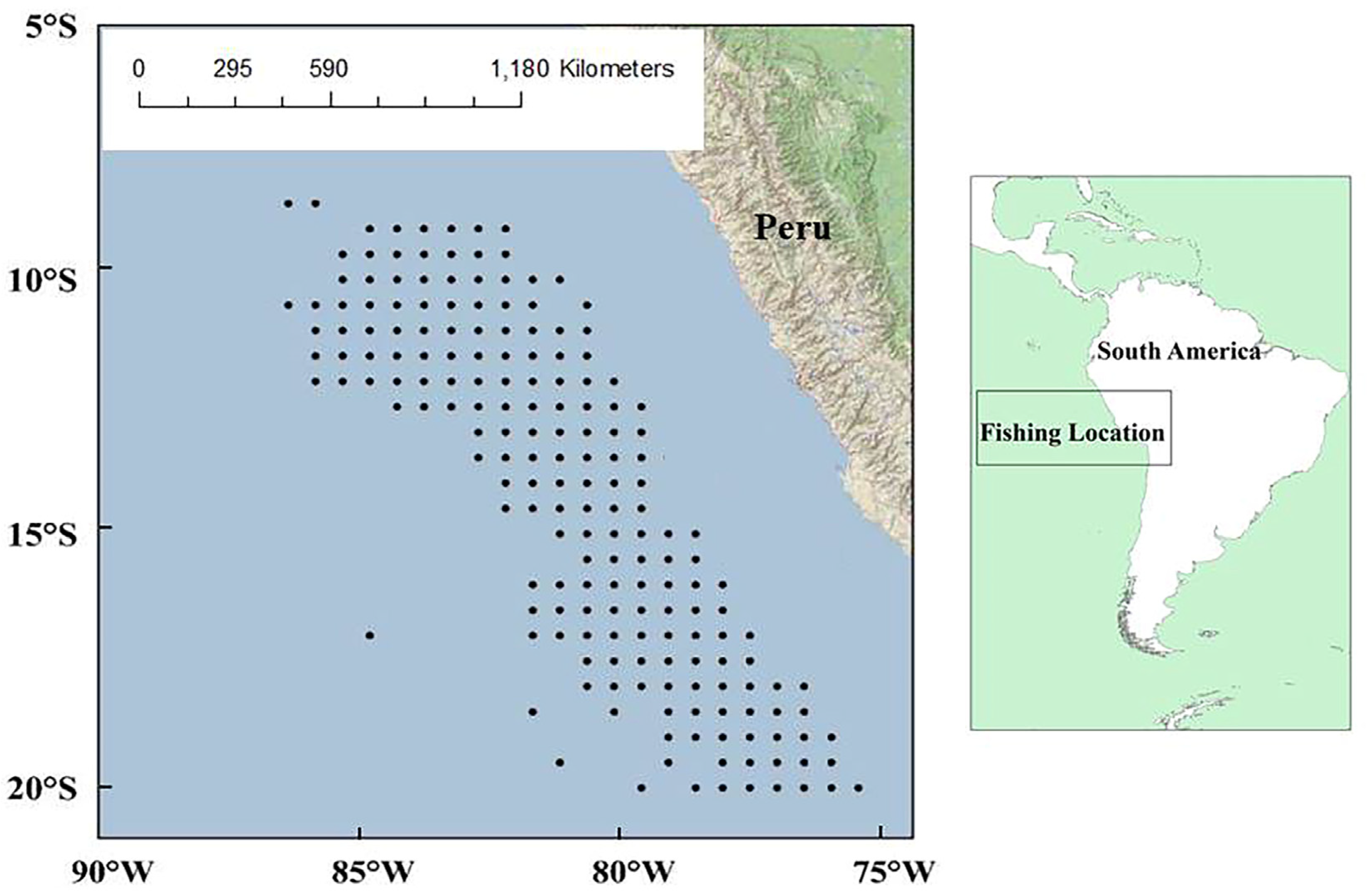
2.1. Jumbo Flying Squid Fisheries Data

We use the commercial fisheries data of jumbo flying squid in 2015 provided by the National Data Center for Distance-Water Fisheries of China (NDCDF), Shanghai Ocean University. The fishing locations for jumbo flying squid in the southeast Pacific Ocean off Peru (8°~20° S, 90°~75° W) are shown in Figure 1.
The fisheries data for jumbo flying squid in the southeast Pacific Ocean off Peru include information such as catch (tons), fishing date (year and month), fishing locations (latitude and longitude), and fishing effort (fishing days). These data are organized into daily databases and grouped based on a spatial resolution of 0.5°.
All Chinese squid-jigging vessels used for fishing are adaptations of the same type. They are equipped with identical engine power (120 kW), squid-attracting lamp (112 kW) with 16 squid-jigging machines, and fishing equipment. These vessels exclusively conduct fishing operations during nighttime [18]. Given that the Chinese squid-jigging vessels have similar characteristics and fishing practices, catch per unit effort (CPUE) became a dependable measure to assess the abundance of squid on the fishing grounds [19]. In this study, the monthly CPUE within a 0.5° × 0.5° grid cell is calculated using the equation provided by Cao et al. (2009) [1].
C P U E y m i j = Σ C ( y m i j ) Σ E ( y m i j )
where C P U E y m i j , Σ C ( y m i j ) , and Σ E ( y m i j ) are the monthly nominal CPUE (tons [t]/day [d]), the total catch for all fishing vessels operating within a specific fishing grid and the cumulative fishing effort of all vessels within that same grid at longitude i and latitude j in month m and year y.

2.2. Environmental Data

We select Moderate-Resolution Imaging Spectroradiometer (MODIS) Aqua and Terra sea surface temperature level 3 inversion image data (in days) from January to December 2015 to determine the environment feature. The website for the SST data is from NASA GSFC water color data network (https://oceancolor.gsfc.nasa.gov/ (accessed on 3 September 2023)).
The amount of the daily SST image data is, in total, 730 (in NetCDF format), and the initial spatial resolution of the image is 0.0416 ° × 0.0416 ° . We normalize these data based on Formula (2).
P ( i , j ) = M A X S S T ( i , j ) M A X M I N ,
where P ( i , j ) represents the normalized SST value at longitude i and latitude j, and S S T ( i , j ) represents the original SST value at the same coordinates; MAX denotes the maximum daily SST value recorded in 2015, while MIN represents the minimum daily SST value observed in the same year.
After normalizing daily SST images, we divide them into sub-images measuring 0.5° × 0.5°, which correspond to each CPUE grid. Each sub-image is then represented by 12 × 12 pixels. In total, we obtain 267,180 sub-images for the study area. However, since some of these sub-images do not fully cover a 0.5° × 0.5° fishing area, we perform image fusion using the following formula:
P ( i , j ) = P T i , j , P A i , j = 0 , P T i , j 0 P A i , j   , P A i , j 0 , P T i , j = 0 0 , P A i , j ,   P T i , j = 0 P T i , j + P A i , j 2 , P A i , j ,   P T i , j 0 ,
where P ( i , j ) represents the daily SST value at coordinates ( i , j ) after fusion; P A i , j represents the MODIS-Aqua SST value; and P T i , j   represents the MODIS-Terra SST value. After fusion, we receive a total of 56,468 sub-images. We also drop the sub-images with more than 50% pixels of zero values ( P ( i , j ) = 0 ). Finally, only 46,524 sub-images are left. The above preprocessing was based on MATLAB (2021 version) software.

2.3. SST Feature Extraction Based on the DCEC Model
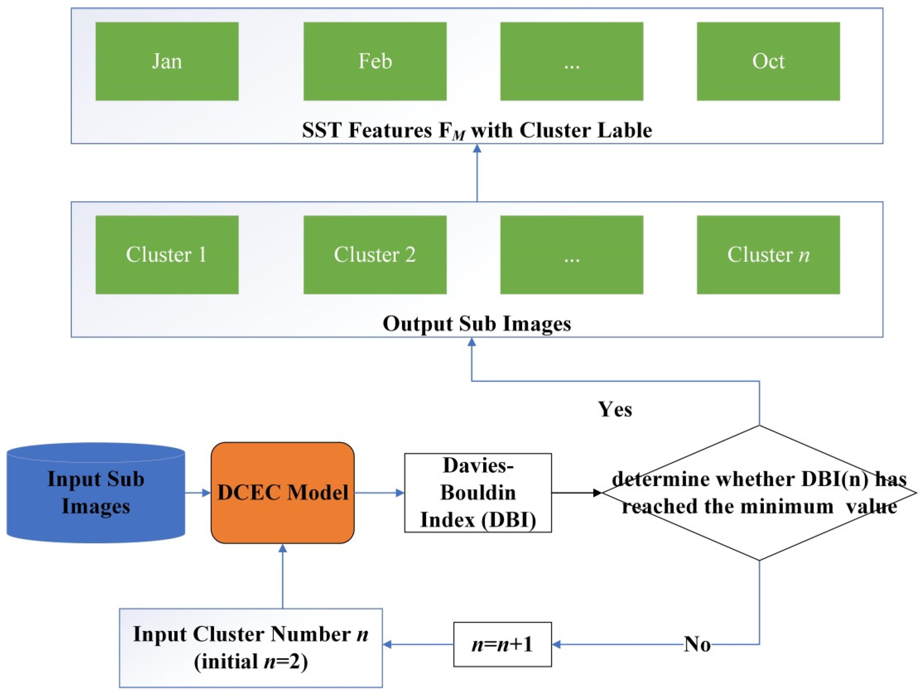
The deep convolutional embedded clustering (DCEC) model is a deep learning-based clustering algorithm proposed in the field of machine learning. It combines the features of convolutional neural networks (CNNs) and autoencoders to perform both dimensionality reduction and clustering in an unsupervised manner. The structure of the DCEC model incorporates a deep embedded clustering framework, and could be found in the published paper of Guo (2017) [20].
The DCEC model autoencoders consist of two main parts: the encoder and the decoder. The encoder’s purpose is to transform the input data into a lower-dimensional representation, while the decoder is responsible for reconstructing the output data from this lower-dimensional representation. Both the encoder and decoder layers consist of 3 convolutional layers, and the stride is set to 2. The input data x is passed through the encoder, after which it is flattened into a one-dimensional feature representation following the 3 convolutional layers. The output feature from the encoder is then received by the decoder and the clustering layer. The decoder then reconstructs images from the compressed latent space representation by minimizing the reconstruction error. The clustering layer assigns the images to different clusters based on the selection of the number of clusters. The result, denoted as x’, is the reconstructed images produced by the decoder. The optimal clustering results for x are generated by the clustering layer. The reconstructed images x’ are assigned cluster labels based on the optimal clusters and organized into monthly groups. The final monthly SST feature for each CPUE grid are determined by identifying the assigned cluster labels of the images that appear with the highest frequency within a month.
In this paper, the source code for the DCEC model is downloaded from the GitHub repository located at https://github.com/XifengGuo/DCEC (accessed on 15 September 2023).
The selection of the number of clusters is crucial during the training of the DCEC model. A small number of clusters may result in limited diversity in the extracted SST feature information, while a large number of clusters can lead to redundancy and increased computational costs. We utilize the Davies–Bouldin index (DBI) to determine the optimal number of clusters [21]. The DBI is calculated as the average of the maximum ratio of the within-cluster distance and the between-cluster distance for each cluster. A smaller DBI value indicates higher similarity among samples within clusters. The formula for calculating the DBI is as follows:
D B I = 1 N i = 1 , j i N m a x S i ¯ + S j ¯ W i W j 2 ,
where N is the number of clusters; S i ¯ (or S j ¯ ) is the average distance of all points in cluster   i (or j ) to the centroid of cluster   i   ( o r   j ) ; W i W j 2 is the distance between the centroids of clusters i and j .
Based on the DCEC model and the DBI index, the SST feature extraction process is performed as follows (Figure 2):
(1)
The 46,524 SST sub-images are put into the DCEC model, and the initial cluster number n is set as 2;
(2)
The input images pass through the autoencoders, and the clustering layer assigns the images to different clusters;
(3)
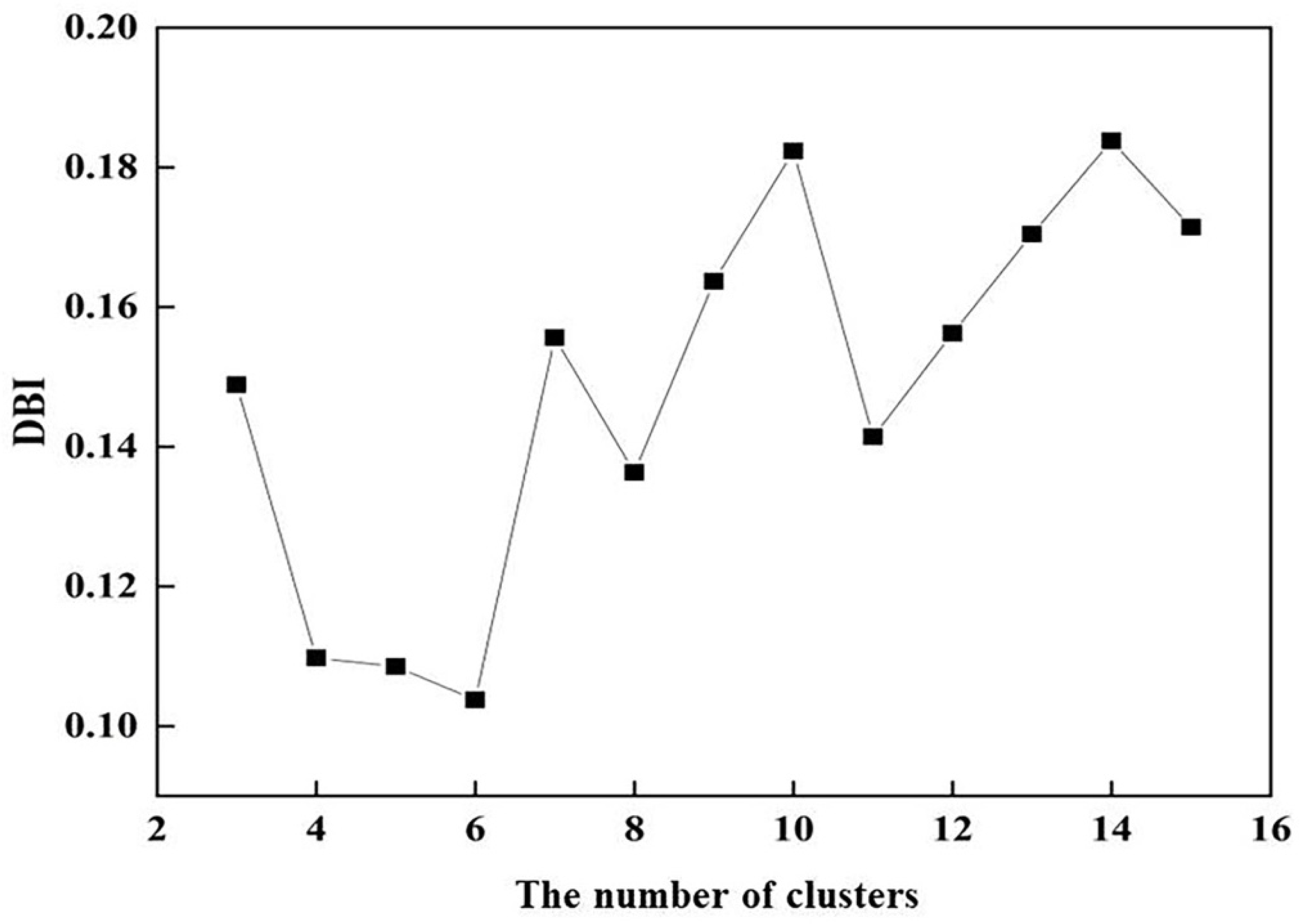
The Davies–Bouldin index (DBI) is calculated to test the similarity among images within clusters;
(4)
The cluster number is set as n + 1, and the above steps (2) and (3) continue until DBI has reached the minimum value, and then the optimal number of clusters is determined.
(5)
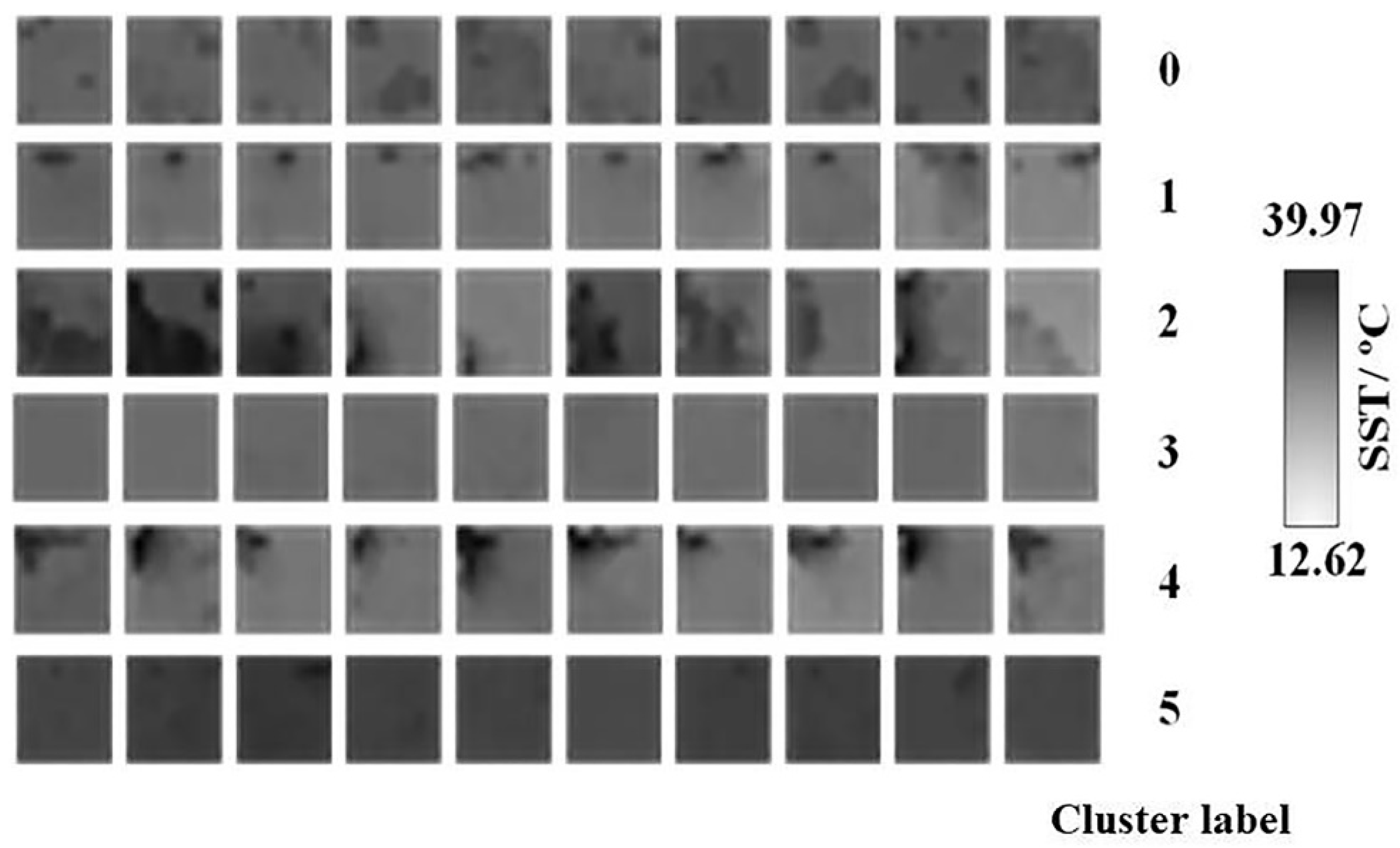
The output images are assigned the cluster labels based on the optimal clusters and organized into monthly groups.
(6)
For each CPUE grid, the SST feature F M for the Mth month is determined by identifying the assigned cluster labels of the images that appear with the highest frequency within a month. This is expressed as follows:
F M = M o d e { c 1 , c 2 , c k , c n }
where F M represents SST feature for the Mth month. The term “Mode” is a statistical term that refers to the value that occurs most frequently among the images in the Mth month; c 1 ,   c 2 ,   c k , c n are the labels of images in that specific month. The above feature extraction process is performed based on Python 3.7.

2.4. GAM Construction and Verification

Generalized Additive Model (GAM) is a data-driven model widely used in fishery research due to its nonparametric nature and high flexibility [22]. It employs smooth functions to establish the relationship between the expected response variables and each explanatory variable and allows for the independent analysis of the nonlinear impact of each explanatory variable on the response variables.
In this study, three types of Generalized Additive Models (GAMs) were developed using the controlled variable method.
(1)
Basic GAM, which uses the traditional monthly average SST value to predict CPUE. To address the issue of underfitting in fishery forecasting models caused by relying solely on a single factor, an additional variable—the monthly average concentration of chlorophyll-a (Chl a)—is included in the model. Chl a has been identified as an important factor influencing squid fishing grounds. We downloaded the 0.5 ° × 0.5 °   monthly average value of Chl a concentration from the NOAA website (https://oceanwatch.pifsc.noaa.gov/ (accessed on 3 September 2023)) from January to December in 2015.
The basic GAM was shown in Formula (6):
ln C P U E = s C h l   a + s S S T ,
where C P U E represents the monthly catch per unit effort; C h l   a represents the monthly average value of chlorophyll a concentration; S S T represents the monthly average value of sea surface temperature; the s function represents the natural cubic spline smoothing function. The error distribution of the model is assumed to be Gaussian distribution.
(2)
Improved GAM, which integrates the extracted SST features along with the average Chl a value. This approach aims to enhance the predictive capability of the model by incorporating more comprehensive and refining representations of the SST monthly feature. The improve GAM model expression is shown in Formula (7):
ln C P U E = s C h l   a + s F M ,
where C P U E represents the monthly catch per unit effort; C h l   a represents the monthly average of the concentration of chlorophyll a; F M represents the monthly SST extracted feature value; s ( · ) represents the natural cubic spline smoothing function. The error distribution of the model is assumed to be Gaussian distribution.
(3)
Full GAM, which includes both the traditional monthly average SST value and the extracted SST features, along with the average Chl a value. We tend to test the improvement of using full variables on the predictive capability of the models. The full GAM model expression is shown in Formula (8):
ln C P U E = s C h l   a + s S S T + s F M
where C P U E represents the monthly catch per unit effort; C h l   a represents the monthly average of the concentration of chlorophyll a; F M represents the monthly SST extracted feature value; s ( · ) represents the natural cubic spline smoothing function. The error distribution of the model is assumed to be Gaussian distribution.
The three types of models described above are constructed using a ten-fold cross-validation approach to divide the dataset into a training set (S) and a test set (T). The training set (S) is used to train and fit the GAM model while simultaneously recording the evaluation parameters of the explanatory variables. The test set (T) is kept separate and used solely for calculating the prediction error of the GAM model.
In this study, the goodness of the model is measured using AIC (Akaike Information Criterion). A lower AIC value indicates a higher goodness of fit for the model. It provides a comparative measurement to assess the relative performance and accuracy of different models. Furthermore, the Mean Squared Error (MSE) is calculated to evaluate the prediction accuracy of the model. The MSE measures the average squared difference between the measured values and the predicted values. On the same test set, a smaller MSE indicates a better prediction accuracy, as it reflects a smaller average discrepancy between the predicted values and the actual measured values. The calculation formula of MSE is shown in (9):
M S E = 1 m i = 1 m C P U E i ^ C P U E i 2 ,
where C P U E i ^ represents the predicted CPUE value of the model; C P U E i represents the measured CPUE value of the sample; m represents the number of samples in the test set.
To further evaluate the prediction effect of the model, the Pearson correlation coefficient (r) is calculated to quantify the strength and direction of the linear relationship between the measured values and the predicted values. The calculation formula of r is shown in (10):
r C P U E i ^ , C P U E i = C o v C P U E i ^ , C P U E i V a r C P U E i ^ V a r C P U E i ,
where   r ( C P U E i ^ , C P U E i ) represents the relationship between the measured values and the predicted values; C o v C P U E i ^ , C P U E i is the covariance of the predicted value and the measured value; Var[ C P U E i ^ ] is the variance of the predicted value; and Var[ C P U E i ] is the variance of the measured value.
The influence of the explanatory variables in the GAM model on the response variables is verified using a joint hypothesis F test. Following the F test, if the p-value associated with an explanatory variable is less than 0.05, it indicates that the variable has a significant impact on the response variable. Based on this result, the explanatory rate of each variable is compared and analyzed. We also draw the response curve for visualizing the relationship between the explanatory variables and the CPUE of jumbo flying squid.

3. Results

3.1. SST Feature Extraction Results Based on DCEC Model

The DBI value reaches its minimum when the cluster number n is 6, as shown in Figure 3. Therefore, the optimal cluster number is 6.
We randomly selected 10 sub-images from each of the six clusters to show the SST distribution pattern, as shown in Figure 4.
In Figure 4, when F M is 0, there is an intersection of cold and warm currents, resulting in an intricate intersection pattern. When F M is 1 and 4, a cold current is observed from south or southeast. On the other hand, an F M of 2 indicates a cold current converging with a warm current from the southwest. Meanwhile, when the SST spatial distribution pattern is characterized by F M s of 3 and 5, the temperature distribution appears relatively uniform. The lowest temperature is observed when the F M value is 3, while a relatively higher temperature is seen when the F M value is 5.

3.2. Model Evaluation Results

The AIC and MSE values, as well as the correlation coefficients r between the predicted CPUE values and the measured values of the basic GAM, the improved GAM, and the full GAM, are shown in Table 1.
Based on Table 1, the improved and full GAM models show that the AIC value is 9.72% and 27.4% lower than the basic GAM model. Additionally, the MSE decreases by 31.1% and 46.6%. The correlation coefficient r increases to 0.60 in the improved GAM and 0.67 in the full GAM, indicating a stronger correlation compared to the basic GAM.

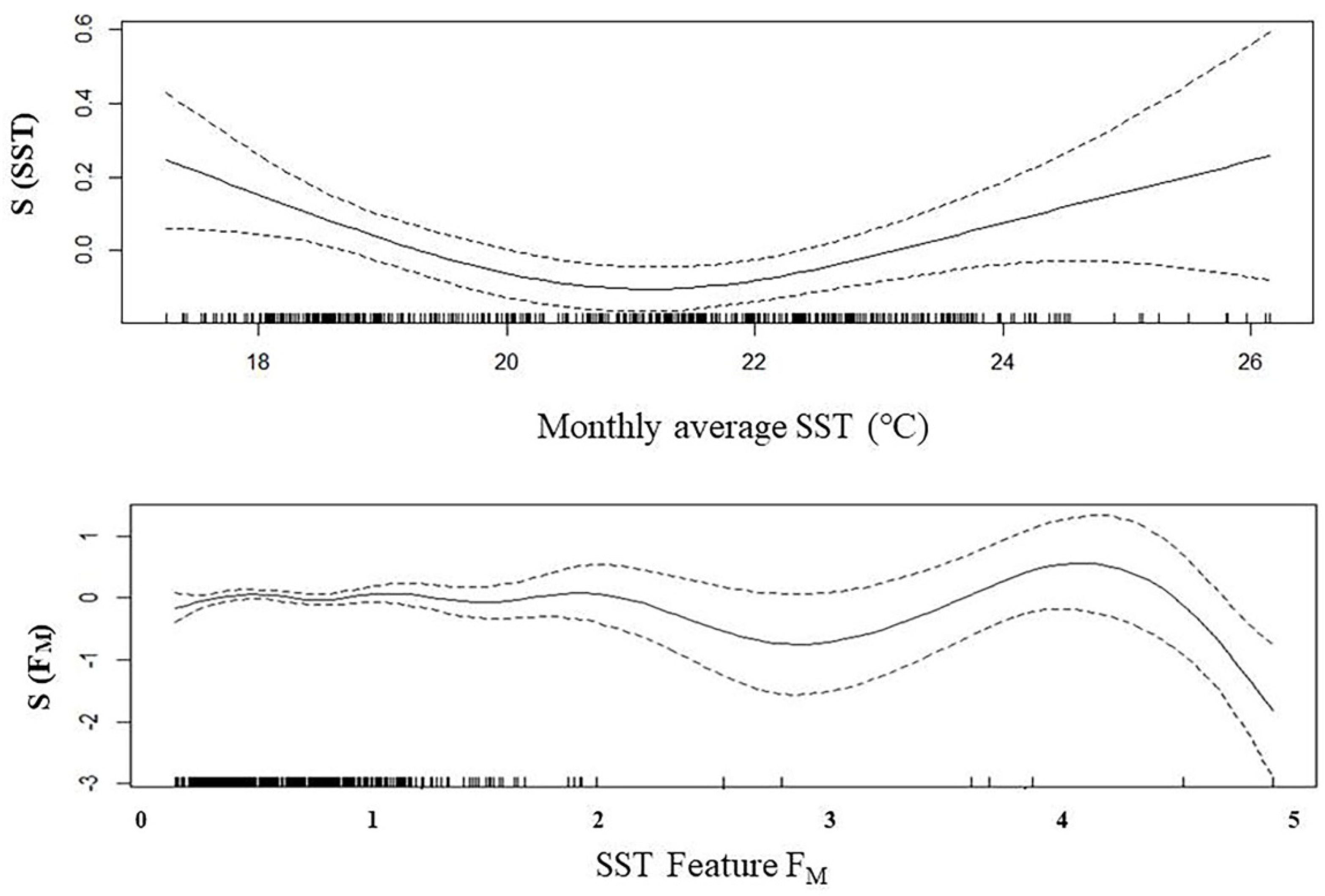
3.3. The Influence of the Explanatory Variables

Table 2 presents the p-values for the F test and variable interpretation rate in the basic, improved, and full GAM.
The results reveal that the p values for SST, F M , and Chl a are less than 0.05, indicating the significant impact of these variables on the response variable. Irrespective of whether F M   is used alone or combined with the Chl a factor in the improved GAM, the factor interpretation rate of the improved GAM consistently surpasses that of the basic GAM. This underscores the significant influence of the extracted F M value in this study. In the full GAM, the factor interpretation rate of the full variables increased to 34.54%, which demonstrates that using all the features together can further improve model performance.
Figure 5 displays the response curve illustrating the relationship between the average SST and the response variable for the basic GAM and the relationship between the F M value and the response variable for the improved GAM.
In the basic model, the response curve depicts a distribution of high CPUE values at relatively low temperatures. The average SST between the upper and lower 95% confidence interval dashed lines ranges from 19 to 23 °C. However, it is not possible to accurately determine the optimal temperature pattern for jumbo flying squid abundance. In the improved model, high CPUE values are observed when F M is 0, 1, 2, and 4, while a relatively low CPUE value is observed when F M is 3 or 5. These results suggest that the intersection of cold and warm ocean currents could have a substantial effect on the abundance of jumbo flying squid.

4. Discussion

4.1. The Effectiveness of the Model in Extracting SST Features

The six clusters of the SST sub-images extracted based on DCEC and DBI showed unique temperature distribution patterns. They exhibit similarity within each cluster and comparability between different clusters. The effectiveness of the model in extracting ocean features relies on several factors, such as model performance, data quality and quantity, and complexity of the features [23]. Firstly, the DCEC model combines the power of deep convolutional autoencoders, which are neural networks used for dimensionality reduction, with clustering algorithms to perform joint feature learning and clustering simultaneously [24,25]. This model has shown promising results in various image-related tasks, such as object recognition and segmentation, remote sensing image classification, data dimensionality reduction, and image noise reduction [12,26,27,28]. In comparison to traditional feature extraction methods, the high-level features extracted by the DCEC model provide better amplitude and phase information. In this study, the DCEC model automatically learns hierarchical representations from the 46,524 daily SST sub-images and processes the high-dimensional ocean data and extracts the meaningful low-dimensional representations. Secondly, MODIS-Aqua and MODIS-Terra SST three-level inversion image data have the relatively high resolution of approximately 1 km, and the MODIS instruments undergo regular calibration processes to ensure the accuracy and consistency of the data [12]. We also make the performed image fusion to ensure that each sub-image can cover each CPUE fishing area, so that each type of image classification result can reflect the monthly dynamics of SST in a small range (0.5° × 0.5°). Lastly, the daily SST sub-images from the southeast Pacific Ocean off Peru over the course of a year may include complex and diverse features. We use DBI to determine the optimal number of clusters, as it produces a single numerical value that indicates the quality of clustering, making it easy to understand and compare different clustering solutions [29]. Our results show that each type of the clusters determined by DBI reflect distinctive patterns of cold and warm currents, showcasing the potential to capture important spatial and temporal information about the ocean current dynamics. On the above basis, this study demonstrates the capability of the DCEC model combined with DBI in extracting ocean SST features.

4.2. The Improvement of GAM Based on the Ocean Feature Extraction Approach

Our study showed that applying an ocean feature extraction approach in the GAM models led to improved prediction accuracy compared to using basic GAM models. This improvement can be attributed to two key factors. First, as discussed above, the ocean feature extraction approach effectively captured the SST distribution pattern. By considering the fine-grained details and spatial variations of the SST data, the GAM models were able to better understand and model the underlying relationships between the SST dynamic and the abundance distribution of jumbo flying squid. Second, the ocean feature extraction approach mitigated the smoothing effect caused by using monthly average SST values. Monthly averages tend to smooth out the inherent variability in SST, potentially leading to an oversimplified representation of the true SST distribution. By extracting ocean features, which likely include more granular and localized SST information, the GAM models were able to capture and incorporate these smaller-scale variations into their predictions. As a result, the improved models were better equipped to account for the true complexity and heterogeneity of the SST distribution pattern, leading to enhanced prediction accuracy.
Our results also demonstrate that using both F M and average SST together can further improve model performance, as they provide complementary information that captures different aspects of the ocean SST environment. F M provides valuable insights into the complex dynamics of the ocean SST and helps the model better understand the underlying patterns and relationships in the data. On the other hand, average SST is a simple but important metric that represents the overall thermal conditions of the ocean surface. By combining ocean feature extraction features with average SST, the model can leverage both detailed and high-dimensional information from the extracted features and the holistic view provided by the average SST. This combination allows the model to make more informed and accurate predictions by considering a wider range of oceanic characteristics and their interactions. In essence, the synergy between the detailed features and the overall SST can lead to a more comprehensive understanding of the ocean system and ultimately improve the model’s performance.
This study found that the extracted SST features, F M , have a significant impact on the abundance distribution of jumbo flying squid in the southeast Pacific Ocean off Peru. The distribution and migration of jumbo flying squid are influenced by various factors, including the SST and ocean currents. The F M features extracted in this study directly represent the changes in these factors. Based on the images of each F M cluster, we could distinguish the regions with high or low temperature and find the intersection of cold and warm currents. The relationship curve between the F M and CPUE of jumbo flying squid showed that the high catch rate was concentrated in the intersection area of warm and cold currents when F M was 0, 1, 2, and 4, while the low catch rate was concentrated in the area with uniform high or low temperature distribution when F M was 3 and 5. The mixing of warm and cold currents creates nutrient-rich waters, attracting an abundance of prey species, such as small fish and plankton, which are the main food sources for squid. Additionally, the varying temperatures in this region create favorable conditions for squid eggs and larvae to develop. The F M feature also indicated that SST and ocean currents play a crucial role in shaping the movement and distribution of jumbo flying squid. Previous studies have shown that jumbo flying squid have specific SST preferences and are often associated with areas where water temperature levels are within their preferred range (18~22 °C) [9]. Suitable hydrological conditions can influence squid behavior, aggregations, and foraging opportunities. In addition, the squid populations tend to follow oceanic currents, which provide them with a means of transportation and facilitate their dispersal over large distances [30,31]. In the southeast Pacific Ocean off Peru, the main oceanic currents that significantly influence the region’s hydrodynamics and marine ecosystem include (1) the Humboldt Current, which is a cold, nutrient-rich current that flows northward along the western coast of South America. It is a major upwelling system, bringing deep, cold, and nutrient-rich waters to the surface, which support a highly productive ecosystem; (2) the Peru-Chile Current, which is an extension of the Humboldt Current and flows parallel to the coast of Peru and Chile. It transports the cold, nutrient-rich waters further north along the coast, allowing for sustained upwelling and supporting a diverse range of marine life; (3) the South Equatorial Current, which flows eastward in the southern hemisphere between approximately 5° S and 20° S latitude. While it does not directly impact the coast of Peru, it influences the circulation patterns in the wider eastern Pacific region, including the southeastern Pacific Ocean off Peru [32,33]. These currents drive the unique hydrological characteristics in the southeast Pacific Ocean off Peru, such as the cold waters associated with upwelling events. The combination of these currents and upwelling processes creates a highly productive marine ecosystem that supports the jumbo flying squid [34,35,36].
Overall, our study highlighted the importance of considering domain-specific ocean feature extraction methods in GAM modeling, particularly when dealing with spatially varying and fine-grained data like SST. These findings have implications for similar modeling scenarios, where capturing and incorporating detailed patterns and mitigating potential smoothing effects can lead to improved prediction performance.

4.3. Prospect

Although the improved GAM model shows better prediction accuracy compared to the basic GAM model, the extent of improvement is not significant. There are several main shortcomings and areas that need further improvement. (1) There are two sources of images, MODIS-Aqua and MODIS-Terra, which are used for fusion in certain areas. In the data preprocessing stage, image data with invalid pixels exceeding 50% are discarded. However, this step partially disrupts the time correlation of the SST image data and reduces the original data space. Consequently, it can lead to a loss of precision in the feature extraction process of the DCEC model and subsequently impact the fitting and prediction accuracy of the improved GAM model. To address these issues, we need to explore the development of a multi-source data fusion method, which could generate more complete SST image data and minimize experimental errors; (2) The fishing ground is a complex system influenced by various factors, such as dissolved oxygen, thermocline, and ocean currents. In this study, the DCEC model was solely employed to extract characteristics from SST data, resulting in limited improvement in the GAM. For future research, it is crucial to integrate multiple factors to extract more dynamic temporal and spatial characteristics of the marine environment; (3) As the new generation of artificial intelligence (AI) continues to evolve, big data and statistical machine learning (SML) technologies are becoming more deeply integrated to significantly improve the processing and forecasting accuracy of fishery models. Examples include the applications of SML in fishery weather simulation and forecasting, such as generating synthetic weather data, developing weather forecast models, and developing extreme weather warning systems [37]. By analyzing historical data, SML algorithms can learn the patterns and relationships between weather variables and then use these patterns and relationships to predict future weather conditions. In this study, we only exacted the SST patterns based on the AI model and used the patterns in the traditional GAM for forecasting the fishery ground. In the future, we may try to use SML to directly analyze the patterns and the associations among multiple variables to make fishery predictions.

5. Conclusions

This study proposed a method for extracting marine environmental features based on the DCEC model combined with the GAM model to forecast the jumbo flying squid in the southeast Pacific Ocean off Peru. We used the extracted SST feature F M to construct an improved GAM model and the monthly average value of SST to construct a basic GAM model. The comparison results of the two types of models show that (1) The SST feature clusters obtained through the DCEC model could capture the SST monthly variations within 0.5° × 0.5°; (2) The GAM models with F M outperform the models with the traditional monthly average SST in terms of predictive accuracy; (3) Using both F M and average SST together can further improve model performance. The results prove the effectiveness of DCEC combined with DBI in marine feature extraction and suggest that using the ocean environment feature extraction based on machine learning could improve the fishery forecasting models for jumbo flying squid, making them more accurate and reliable.

Author Contributions

Conceptualization, T.Z. and H.Y.; methodology, T.Z. and J.X.; software, T.Z. and J.X.; validation, L.S., H.Y. and Z.Y.; formal analysis, L.S. and T.Z.; investigation, T.Z. and J.X.; resources, L.S., W.Y. and H.Y.; data curation, T.Z. and W.Y.; writing—original draft preparation, T.Z.; writing—review and editing, L.S., H.Y. and Z.Y.; visualization, J.X.; supervision, H.Y. and W.Y.; project administration, L.S.; funding acquisition, H.Y. All authors have read and agreed to the published version of the manuscript.

Funding

This research was funded by the National Key R&D Program of China: 2023YFD2401303; the National Natural Science Foundation of China: 32273185; the Special Foundation for Science and Technology Development of Shanghai Ocean University: A2-2006-22-200204; and the Open Fund for Key Laboratory of Sustainable Exploitation of Oceanic Fisheries Resources in Shanghai Ocean University: A1-2006-23-200207.

Institutional Review Board Statement

The animal study protocol was approved by the Institutional Review Board (or Ethics Committee) of Shanghai Ocean University (protocol code SHOU-DW-296-001 and date of approval is 10 April 2016).

Data Availability Statement

The fishery data presented in this study are available on request from the corresponding author. The data are not publicly available due to trade secrets of the fishing vessel company.

Acknowledgments

The authors wish to thank Bo Song, China Institute of FTZ Supply Chain, Shanghai Maritime University, Shanghai, China, for suggesting improvements in the language. The authors also wish to thank Shuyan Sun, Changchun University of Technology, Changchun, Jilin, China, for improving the quality of the figures in the manuscript.

Conflicts of Interest

The authors declare no conflicts of interest.

References

  1. Cao, J.; Chen, X.J.; Chen, Y. Influence of surface oceanographic variability on abundance of the western winter-spring cohort of neon flying squid Ommastrephes bartramii in the NW Pacific Ocean. Mar. Ecol. Prog. Ser. 2009, 381, 119–127. [Google Scholar] [CrossRef]
  2. Chen, X.J.; Tian, S.Q.; Chen, Y.; Liu, B.L. A modeling approach to identify optimal habitat and suitable fishing grounds for neon flying squid (Ommastrephes bartramii) in the Northwest Pacific Ocean. Fish. Bull. 2010, 108, 1–14. [Google Scholar]
  3. Chen, X.; Lu, H.; Liu, B.; Chen, Y. Age, growth and population structure of jumbo flying squid, Dosidicus gigas, based on statolith microstructure off the Exclusive Economic Zone of Chilean waters. J. Mar. Biol. Assoc. U. K. 2011, 91, 229–235. [Google Scholar] [CrossRef]
  4. Waluda, C.M.; Rodhouse, P.G. Remotely sensed mesoscale oceanography of the Central Eastern Pacific and recruitment variability in Dosidicus gigas. Mar. Ecol. Prog. Ser. 2006, 310, 25–32. [Google Scholar] [CrossRef]
  5. Waluda, C.M.; Yamashiro, C.; Rodhouse, P.G. Influence of the ENSO cycle on the light-fishery for Dosidicus gigas in the Peru Current: An analysis of remotely sensed data. Fish. Res. 2006, 79, 56–63. [Google Scholar] [CrossRef]
  6. Igarashi, H.; Ichii, T.; Sakai, M.; Ishikawa, Y.; Toyoda, T.; Masuda, S.; Sugiura, N.; Mahapatra, K.; Awaji, T. Possible link between interannual variation of neon flying squid (Ommastrephes bartramii) abundance in the north pacific and the climate phase shift in 1998/1999. Prog. Oceanogr. 2015, 150, 20–34. [Google Scholar] [CrossRef]
  7. Montecalvo, I.; Le Billon, P.; Arsenault, C.; Schvartzman, M. Ocean predators: Squids, Chinese fleets and the geopolitics of high seas fishing. Mar. Policy 2023, 152, 105584. [Google Scholar] [CrossRef]
  8. Xu, L.L.; Chen, X.J.; Wang, J.T. Inter-annual variation in abundance index of Dosidicus gigas off Peru during 2003 to 2012. J. Shanghai Ocean. Univ. 2015, 24, 280–286. [Google Scholar]
  9. Paulino, C.; Segura, M.; Chacón, G. Spatial variability of jumbo flying squid (Dosidicus gigas) fishery related to remotely sensed SST and chlorophyll-a concentration (2004–2012). Fish. Res. 2016, 173, 122–127. [Google Scholar] [CrossRef]
  10. Hu, G.; Boenish, R.; Gao, C.; Li, B.; Chen, X.; Chen, Y.; Punt, A.E. Spatio-temporal variability in trophic ecology of jumbo squid (Dosidicus gigas) in the southeastern Pacific: Insights from isotopic signatures in beaks. Fish. Res. 2019, 212, 56–62. [Google Scholar] [CrossRef]
  11. Frawley, T.H.; Briscoe, D.K.; Daniel, P.C.; Britten, G.L.; Crowder, L.B.; Robinson, C.J.; Gilly, W.F. Impacts of a shift to a warm-water regime in the Gulf of California on jumbo squid (Dosidicus gigas). ICES J. Mar. Sci. 2019, 76, 2413–2426. [Google Scholar] [CrossRef]
  12. Zhang, T.; Song, L.; Yuan, H.; Song, B.; Ngando, N.E. A comparative study on habitat models for adult bigeye tuna in the Indian Ocean based on gridded tuna longline fishery data. Fish. Oceanogr. 2021, 30, 584–607. [Google Scholar] [CrossRef]
  13. Song, L.; Li, T.; Zhang, T.; Sui, H.; Li, B.; Zhang, M. Comparison of machine learning models within different spatial resolutions for predicting the bigeye tuna fishing grounds in tropical waters of the Atlantic Ocean. Fish. Oceanogr. 2023, 32, 509–526. [Google Scholar] [CrossRef]
  14. Tian, S.; Chen, X.; Chen, Y.; Xu, L.; Dai, X. Evaluating habitat suitability indices derived from CPUE and fishing effort data for Ommatrephes bratramii in the northwestern Pacific Ocean. Fish. Res. 2009, 95, 181–188. [Google Scholar] [CrossRef]
  15. Ramos, J.E.; Ramos-Rodríguez, A.; Ferreri, G.B.; Kurczyn, J.A.; Rivas, D.; Salinas-Zavala, C.A. Characterization of the northernmost spawning habitat of Dosidicus gigas with implications for its northwards range extension. Mar. Ecol. Prog. Ser. 2017, 572, 179–192. [Google Scholar] [CrossRef]
  16. Barth, A.; Alvera-Azcárate, A.; Licer, M.; Beckers, J.M. DINCAE 1.0: A convolutional neural network with error estimates to reconstruct sea surface temperature satellite observations. Geosci. Model Dev. 2020, 13, 1609–1622. [Google Scholar] [CrossRef]
  17. Medellín-Ortiz, A.; Cadena-Cárdenas, L.; Santana-Morales, O. Environmental effects on the jumbo squid fishery along Baja California’s west coast. Fish. Sci. 2016, 82, 851–861. [Google Scholar] [CrossRef]
  18. Wang, Y.; Chen, X. The Resource and Biology of Economic Oceanic Squid in the World; Ocean Press: Beijing, China, 2005; pp. 79–295. [Google Scholar]
  19. Chen, X.; Zhao, X.; Chen, Y. Influence of El Niño/La Niña on the western winter–spring cohort of neon flying squid (Ommastrephes bartramii) in the northwestern Pacific Ocean. ICES J. Mar. Sci. 2007, 64, 1152–1160. [Google Scholar] [CrossRef]
  20. Guo, X.; Liu, X.; Zhu, E.; Yin, J. Deep clustering with convolutional autoencoders. In Neural Information Processing, Proceedings of the 24th International Conference, ICONIP 2017, Guangzhou, China, 14–18 November 2017; Springer International Publishing: Cham, Switzerland, 2017; pp. 373–382. [Google Scholar] [CrossRef]
  21. Thomas, J.C.R.; Penas, M.S.; Mora, M. New version of Davies-Bouldin Index for clustering validation based on cylindrical distance. In Proceedings of the 32nd International Conference of the Chilean Computer Science Society (SCCC), Temuco, Chile, 11–15 November 2013; IEEE: Piscataway, NJ, USA, 2013. [Google Scholar] [CrossRef]
  22. Guisan, A.; Edwards, T.C.; Hastie, T. Generalized linear and generalized additive models in studies of species distributions: Setting the scene. Ecol. Model. 2002, 157, 89–100. [Google Scholar] [CrossRef]
  23. Himeur, Y.; Rimal, B.; Tiwary, A.; Amira, A. Using artificial intelligence and data fusion for environmental monitoring: A review and future perspectives. Inf. Fusion 2022, 86, 44–75. [Google Scholar] [CrossRef]
  24. Srivastava, N.; Hinton, G.E.; Krizhevsky, A.; Sutskever, I.; Salakhutdinov, R. Dropout: A simple way to prevent neural networks from overfitting. J. Mach. Learn. Res. 2014, 15, 1929–1958. [Google Scholar]
  25. Guo, Y.; Liao, J.; Shen, G. A deep learning model with capsules embedded for high-resolution image classification. IEEE J. Sel. Top. Appl. Earth Obs. Remote Sens. 2020, 14, 214–223. [Google Scholar] [CrossRef]
  26. Duan, Y.; Zheng, X.; Hu, L.; Sun, L. Seismic facies analysis based on deep convolutional embedded clustering. Geophysics 2019, 84, IM87–IM97. [Google Scholar] [CrossRef]
  27. Castellano, G.; Vessio, G. Deep convolutional embedding for digitized painting clustering. In Proceedings of the 2020 25th International Conference on Pattern Recognition (ICPR), Milan, Italy, 10–15 January 2021; IEEE: Piscataway, NJ, USA, 2021; pp. 2708–2715. [Google Scholar] [CrossRef]
  28. van Strien, M.J.; Grêt-Regamey, A. Unsupervised deep learning of landscape typologies from remote sensing images and other continuous spatial data. Environ. Model. Softw. 2022, 155, 105462. [Google Scholar] [CrossRef]
  29. Xiao, J.; Lu, J.; Li, X. Davies Bouldin Index based hierarchical initialization K-means. Intell. Data Anal. 2017, 21, 1327–1338. [Google Scholar] [CrossRef]
  30. Yu, W.; Chen, X. Ocean warming-induced range-shifting of potential habitat for jumbo flying squid Dosidicus gigas in the Southeast Pacific Ocean off Peru. Fish. Res. 2018, 204, 137–146. [Google Scholar] [CrossRef]
  31. Alabia, I.D.; Saitoh, S.I.; Mugo, R.; Igarashi, H.; Ishikawa, Y.; Usui, N.; Kamachi, M.; Awaji, T.; Seito, M. Seasonal potential fishing ground prediction of neon flying squid (Ommastrephes bartramii) in the western and central North Pacific. Fish. Oceanogr. 2015, 24, 190–203. [Google Scholar] [CrossRef]
  32. Taipe, A.; Yamashiro, C.; Mariategui, L.; Rojas, P.; Roque, C. Distribution and concentrations of jumboying squid (Dosidicus gigas) off the peruvian coast between 1991 and 1999. Fish. Res. 2001, 54, 21–32. [Google Scholar] [CrossRef]
  33. Lamy, F.; Rühlemann, C.; Hebbeln, D.; Wefer, G. High- and low-latitude climate control on the position of the southern Peru-Chile Current during the Holocene. Paleoceanography 2002, 17, 16. [Google Scholar] [CrossRef]
  34. Penven, P.; Echevin, V.; Pasapera, J.; Colas, F.; Tam, J. Average circulation, seasonal cycle, and mesoscale dynamics of the Peru Current System: A modeling approach. J. Geophys. Res. Ocean. 2005, 110, 10021. [Google Scholar] [CrossRef]
  35. Ortega, H.; Hidalgo, M. Freshwater fishes and aquatic habitats in Peru: Current knowledge and conservation. Aquat. Ecosyst. Health Manag. 2008, 11, 257–271. [Google Scholar] [CrossRef]
  36. Argüelles, J.; Csirke, J.; Grados, D.; Tafur, R.; Mendoza, J. Changes in the predominance of phenotypic groups of jumbo flying squid Dosidicus gigas and other indicators of a possible regime change in Peruvian waters. In Proceedings of the 7th Meeting of the Scientific Committee of the SPRFMO, La Havana, Cuba, 5–12 October 2019; pp. 5–12. [Google Scholar]
  37. Fu, X.; Zhang, C.; Chang, F.; Han, L.; Zhao, X.; Wang, Z.; Ma, Q. Simulation and forecasting of fishery weather based on statistical machine learning. Inf. Process. Agric. 2023; in press. [Google Scholar] [CrossRef]
Figure 1. The fishing locations for jumbo flying squid in the southeast Pacific Ocean off Peru.
Fishes 09 00081 g001
Figure 2. SST feature extraction process based on the DCEC model and the DBI index.
Fishes 09 00081 g002
Figure 3. The curve representing the relationship between the number of clusters and DBI value.
Fishes 09 00081 g003
Figure 4. SST sub-images within the optimal clusters (10 images were randomly selected for each cluster).
Fishes 09 00081 g004
Figure 5. The relationship curve between the monthly average SST and CPUE in the basic GAM (top); the relationship curve between the SST feature F M and CPUE in the improved GAM (bottom).
Fishes 09 00081 g005
Table 1. AIC, MSE, and correlation coefficients r of the basic, improved, and full GAM.
ModelAICMSEr
Basic GAM9050.0450.21
Improved GAM8170.0310.60
Full GAM6570.0240.67
Table 2. The p-values andvariable interpretation rate in the basic, improved, and full GAM.
ModelModel FactorpInterpretation Rate/%
Basic GAM s C h l   a 0.0007.65
s S S T 0.00111.82
s C h l   a + s ( S S T ) 0.00416.18
Improved GAM s C h l   a 0.0006.84
s F M 0.00015.60
s C h l   a + s ( F M ) 0.00219.76
Full GAM s C h l   a 0.0007.86
s F M 0.00016.37
s S S T 0.00113.59
s C h l   a + s ( F M ) +   s ( S S T ) 0.00234.54
Disclaimer/Publisher’s Note: The statements, opinions and data contained in all publications are solely those of the individual author(s) and contributor(s) and not of MDPI and/or the editor(s). MDPI and/or the editor(s) disclaim responsibility for any injury to people or property resulting from any ideas, methods, instructions or products referred to in the content.

