Deep Learning-Based Fishing Ground Prediction Using Asymmetric Spatiotemporal Scales: A Case Study of Ommastrephes bartramii

Abstract

Selecting the optimal spatiotemporal scale in fishing ground prediction models can maximize prediction accuracy. Current research on spatiotemporal scales shows that they are symmetrically distributed, which may not capture specific oceanographic features conducive to fishing ground formation. Recent studies have shown that deep learning is a promising research direction for addressing spatiotemporal scale issues. In the era of big data, deep learning outperforms traditional methods by more accurately and efficiently mining high-value, nonlinear information. In this study, taking Ommastrephes bartramii in the Northwest Pacific as an example, we used the U-Net model with sea surface temperature (SST) as the input factor and center fishing ground as the output factor. We constructed 80 different combinations of temporal scales and asymmetric spatial scales using data in 1998–2020. By comparing the results, we found that the optimal temporal scale for the deep learning fishing ground prediction model is 15 days, and the spatial scale is 0.25° × 0.25°. Larger time scales lead to higher model accuracy, and latitude has a greater impact on the model than longitude. It further enriches and refines the criteria for selecting spatiotemporal scales. This result deepens our understanding of the oceanographic characteristics of the Northwest Pacific environmental field and lays the foundation for future artificial intelligence-based fishery research. This study provides a scientific basis for the sustainable development of efficient fishery production.

1. Introduction

Accurately predicting the location of fishing grounds holds significant importance for increasing fishing yields and saving fuel costs [1]. The distribution of pelagic species’ fishing grounds is closely related to the climatic and oceanographic environment which they inhabit [2,3,4]. Therefore, fishing ground prediction research typically combines oceanographic remote sensing data to analyze the relationships between marine climate, environmental factors, and species spatial distribution. Linear or nonlinear models are then established for the prediction of fishing grounds. Currently, traditional fishing ground prediction methods such as generalized additive model [5], habitat suitability index model [6], and artificial neural network [7] have achieved notable results. However, with the advent of the big data era in ocean remote sensing and fisheries, traditional methods have struggled to extract valuable, sparse information accurately and efficiently from complex and extensive datasets. It has become challenging to establish highly accurate and robust nonlinear models. Furthermore, the environmental fields that give rise to fishing grounds are complex, dynamic, comprehensive processes with strong temporal and spatial correlations. The traditional methods face bottlenecks in handling the complex spatiotemporal relationships under big data, both in terms of efficiency and accuracy. Deep learning, as an emerging technology in the field of artificial intelligence in recent years, has demonstrated more apparent advantages in handling large-scale image data problems compared to traditional physics-based or statistical information extraction algorithms [8,9]. Moreover, the deep neural network structure and automatic calculation of node weights enable end-to-end learning between input and output. Currently, deep learning has yielded promising results in various applications of the fishery community, such as fish behavior monitoring [10], automatic fish age determination [11], fishery footprint tracking [12], ocean information extraction [13], marine ecology applications [14], environmental monitoring [15,16,17], and the ecology of animal movement [18].

The problem of fishing ground prediction can be viewed as an issue of semantic segmentation in images, where the spatial correlation between environmental field images and fishing ground distribution images is examined over a specific time period. The elaborate U-Net model, first introduced in 2015, was applied to biomedical image segmentation as a deep learning model [19]. It is a well-established artificial neural network for the semantic segmentation of images, and excels in processing spatial features. It represents a convolutional neural network (CNN) that incorporates an encoder–decoder structure, along with skip connections connecting the encoder and the decoder. This architecture enables the enhanced extraction of abstract features and facilitates pixelwise prediction [20]. After appropriate modifications, the U-Net model can be used to establish regression relationships between environmental field images and fishing ground distribution images, thus facilitating fishing ground prediction. In our previous work [21], we conducted preliminary research in this regard, confirming that the U-Net model can be employed for fishing ground prediction, offering an efficient, highly accurate, and stable solution.

In studies concerning spatial distribution relationships, a critical aspect that needs to be addressed is the rational planning of spatiotemporal scales [22]. In different application scenarios, the optimal spatiotemporal scales for different model outcomes may vary [23]. It has been demonstrated in research on the abundance of fishery resources and environmental factors that spatiotemporal scales have a significant impact on predictive model results. Choosing inappropriate spatial scales can lead to significant errors in models. Optimal spatiotemporal scales for models have already been explored in research involving the generalized additive model [24,25], habitat suitability index [26], artificial neural network [27], and other models [28,29]. However, current spatiotemporal scale designs are based on symmetric distributions. This symmetric spatiotemporal scale design may not effectively capture dynamic features, particularly irregular spatial distributions of marine phenomena such as eddies, currents, and fronts, that occur in the ocean. Nonetheless, investigating asymmetric spatiotemporal scales demands extensive, accurate, and efficient data processing, making it challenging for traditional approaches to effectively handle this task. Deep learning, known for its robust data processing and information mining capabilities, offers a solution. Therefore, we employed deep learning techniques, with Ommastrephes bartramii in the Northwest Pacific as a case study, to analyze the impact of asymmetric spatiotemporal scales on fishing ground prediction.

Neon flying squid (Ommastrephes bartramii) holds significant economic value as a cephalopod species in the Northwest Pacific Ocean [1]. This species is characterized by its opportunistic nature, typically completing its life cycle within a year. Previous research has highlighted the influential role of the marine climatic environment in governing the distribution and abundance of the neon flying squid [6]. Among the environmental factors that influence fishing ground variations, sea surface temperature (SST) stands out as one of the primary factors, frequently employed as a contributing factor in constructing fishing ground prediction models [30]. Climate events of varying intensities, such as the Pacific decadal oscillation (PDO) [31] and El Niño-La Niña [32], also regulate the interannual variability in fishing ground distribution. Information pertaining to these decadal climate events is encapsulated within the temporal and spatial variations in SST. Hence, in this study, we utilized SST as the input factor and the distribution of center fishing grounds as the output factor. We designed 80 different asymmetric spatiotemporal scale cases using data spanning 23 years from July to November (1998–2020). The fishing ground prediction model was constructed based on U-Net. By comparing the impacts of different spatiotemporal scales on the model, we selected the optimal spatiotemporal scale for the model and analyzed the sensitivity of the model’s performance to different latitudes and longitudes.

2. Material and Methods

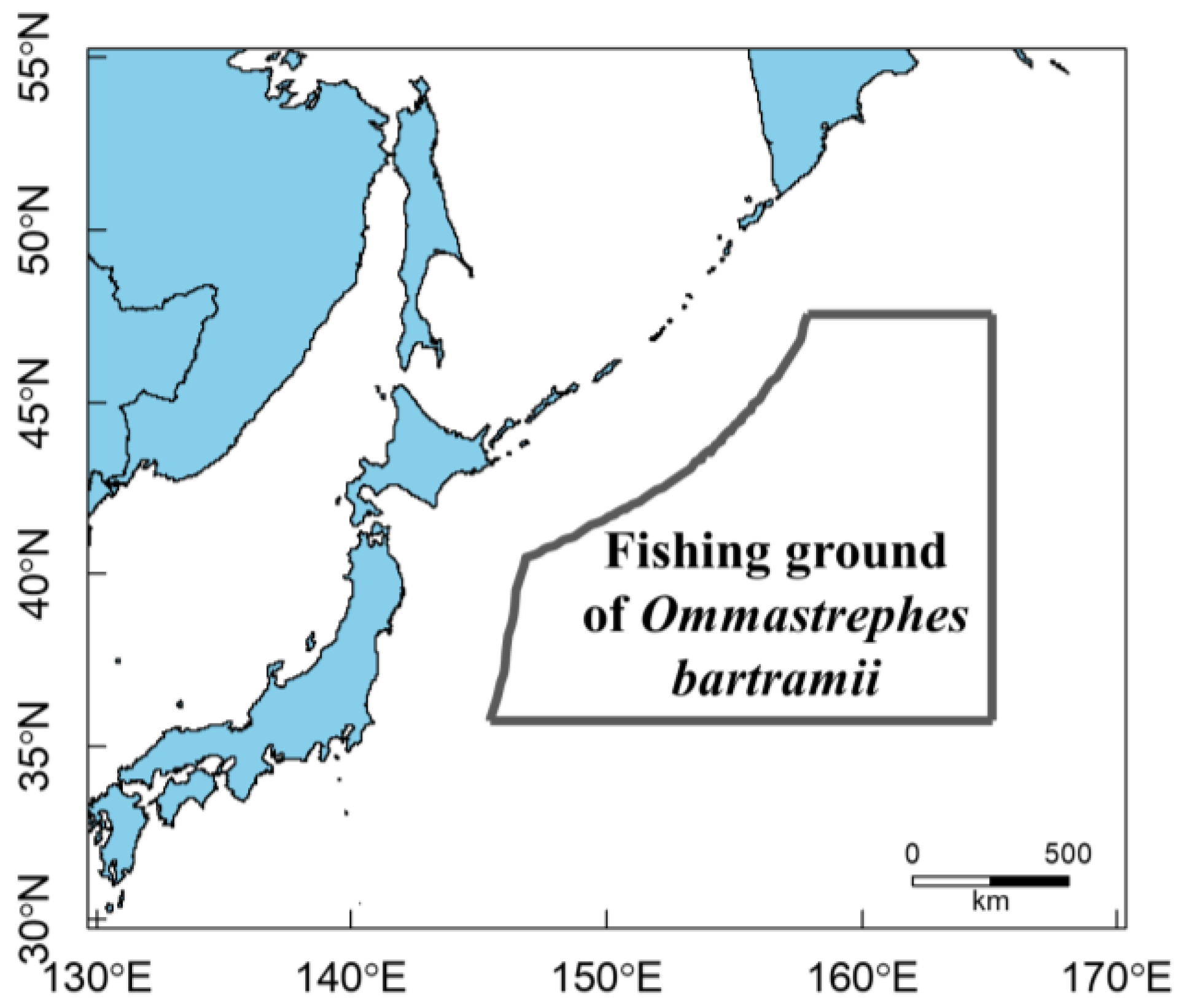
2.1. Data Collection

The commercial fishery data were generously provided by the Chinese Squid-Jigging Technology Group, affiliated with Shanghai Ocean University. The study area encompasses the traditional fishing grounds of Ommastrephes bartramii in the Northwest Pacific Ocean, bounded by coordinates 36° N to 48° N and 145° E to 165° E (Figure 1). This dataset includes detailed information such as fishing dates and locations specified by longitude and latitude at a spatial scale of 0.01°, the numbers of fishing vessels, and the total daily catch (ton). The time range for these records spans the primary fishing season from July to November, covering the years from 1998 to 2020.

The SST data used in this study were sourced from the National Oceanic and Atmospheric Administration (NOAA, https://oceanwatch.pifsc.noaa.gov/, accessed on 7 October 2022). These SST data are available at a temporal scale of 1 day and a spatial scale of 0.05°.

2.2. Data Preprocessing

2.2.1. Definition of the Center Fishing Ground

The resource abundance index of the fishery data was matched with SST data into various spatiotemporal scale cases using the interpolation method (Figure 2). Temporal scales were set at five intervals: 3 days, 6 days, 10 days, 15 days, and 30 days. Spatial scales were set at four intervals: 0.05°, 0.1°, 0.25°, and 0.5°. A total of 80 cases were created by combining asymmetric latitude and longitude scales. Following on from previous research results [21], the catch index [33] for each specific time period within each year was matched with the corresponding SST range, serving as an environmental indicator characterizing the center fishing ground. The SST range of the fishing grounds was defined as the maximum and minimum values observed across all years from 1998 to 2020.

The catch index of the fishing ground has a large degree of dispersion, and the high values of the catch index are relatively concentrated. According to this characteristic, we used the quartile method to classify the fishing ground types according to the SST range corresponding to the catch index of each period. The SST range with index values greater than the upper quartile defines the center fishing ground, labeled 1; otherwise, the non-center fishing ground, labeled 0.

2.2.2. Normalization and Invalid Value Handling

In order to enhance the fitting efficiency of the deep learning model, the SST data were subjected to a normalization process within the range of 0–1. This normalization procedure was performed using the following equation:

$$x=\frac{x_i-x_{\mathrm{m}\mathrm{i}\mathrm{n}}}{x_{\mathrm{m}\mathrm{a}\mathrm{x}}-x_{\mathrm{m}\mathrm{i}\mathrm{n}}}$$

(1)

where x represents the normalized value of the sample, $x_i$ is the original value, and $x_{\mathrm{m}\mathrm{a}\mathrm{x}}$ and $x_{\mathrm{m}\mathrm{i}\mathrm{n}}$ correspond to the maximum and minimum values observed within the sample dataset, respectively. All values that were found to be invalid were consistently replaced with −1 during this normalization process.

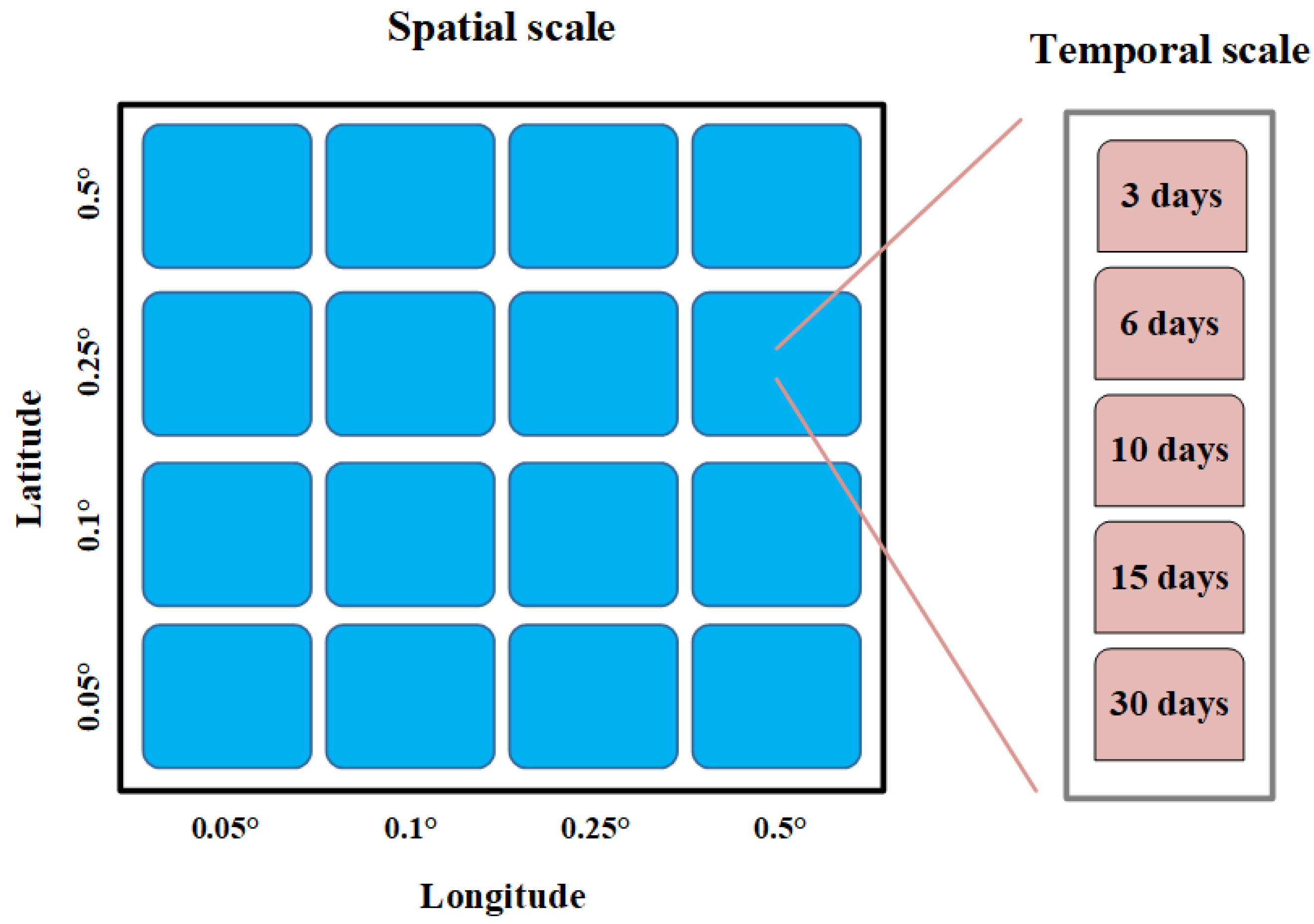
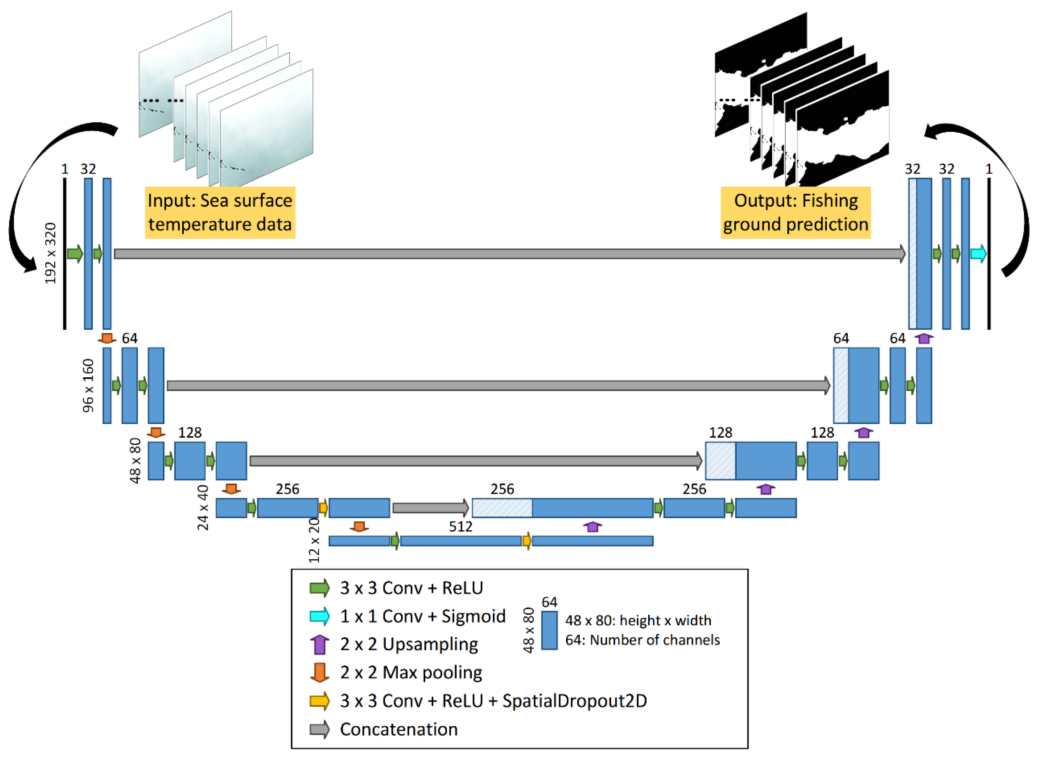
2.3. Prediction Model and Case Design

The fishing ground prediction model, as illustrated in Figure 3, is based on the U-Net model [20]. The U-Net model features a fully convolutional design, comprising two pathways: encoding and decoding. The encoding pathway is responsible for diminishing spatial dimensions while extracting high-level feature data, essential for precise classification. It includes a series of convolutional layers with rectified linear unit (ReLU) activation functions, along with max-pooling operations. The decoding pathway serves to merge abstracted and high-resolution features through a sequence of upsampling and concatenation processes [34]. This segment consists of upsampling operations and convolutional layers with ReLU activation. The model concludes with pixel-level predictions, enabling both classification and regression tasks. As delineated in Figure 3, the model incorporates four upsampling layers, four max-pooling layers, two dropout layers, and four skip connections. The max-pooling and convolution layers employ strides of 2 and 1, respectively. The application of max-pooling effectively reduces the computational load, expands the receptive field of convolutions, facilitates feature learning at multiple scales, and enhances the model’s resilience to noise and clutter. Notably, our preliminary experiments exposed substantial overfitting issues, necessitating a specific remedy. To address this, we introduced the SpatialDropout2D layer [35] to the fourth and fifth convolutional layers. The utilization of this layer proved effective in regulating overfitting. In this study, the dropout rate for the SpatialDropout2D layer is set at 0.75. Considering the model’s binary classification objective, distinguishing center fishing ground from non-center fishing ground, the final convolutional layer utilizes sigmoid activation. Correspondingly, the model employs a binary cross-entropy loss function for the same purpose.

We devised a total of 80 different combinations involving varying temporal and asymmetric spatial scales and subsequently conducted a comparative analysis (Figure 2). It is important to note that a larger spatial scale results in a reduced sample size, while a longer temporal scale corresponds to a smaller number of samples. To maintain a sufficient number of training samples, we imposed restrictions such that the temporal scale does not exceed 30 days and the spatial scale does not exceed 0.5°. As an illustration, consider the following case involving a spatial scale of 0.05° × 0.05° and a temporal scale of 3 days: this configuration yields a sample size of 192 × 320 and a total of 1100 samples (Figure 3).

Following the encoding and decoding processes, the sample size remains unaltered, and the model effectively extracts image features. This feature-rich model is then equipped to provide pixel-level predictions, effectively transforming marine environmental data into detailed fishing ground forecasts. It is imperative to emphasize that this model was specifically tailored for predicting the fishing grounds of the neon flying squid within the Northwest Pacific Ocean [21].

2.4. Case Implementation and Evaluation

In order to assess the model’s performance, we employed several key metrics. The overall accuracy (OA), which is a fundamental indicator, quantifies the ratio of accurately predicted pixels to the total number of pixels. Furthermore, to comprehensively evaluate the model, we calculated the precision, recall, and F1 score of the prediction results. Precision signifies the proportion of correct predictions among all the pixels identified as fishing ground. Recall quantifies the proportion of actual center fishing ground pixels that were correctly predicted. Since there is often a trade-off relationship between precision and recall, we introduce the F1 score, which is the harmonic mean of both precision and recall. These metrics, in accordance with previous research [20], are calculated as follows:

$$\mathrm{O}\mathrm{v}\mathrm{e}\mathrm{r}\mathrm{a}\mathrm{l}\mathrm{l} \mathrm{a}\mathrm{c}\mathrm{c}\mathrm{u}\mathrm{r}\mathrm{a}\mathrm{c}\mathrm{y}:OA=\frac{N_{\mathrm{T}\mathrm{P}}+N_{\mathrm{T}\mathrm{N}}}{N_{\mathrm{T}\mathrm{P}}+N_{\mathrm{T}\mathrm{N}}+N_{\mathrm{F}\mathrm{P}}+N_{\mathrm{F}\mathrm{N}}}\times 100\%$$

(2)

$$\mathrm{P}\mathrm{r}\mathrm{e}\mathrm{c}\mathrm{i}\mathrm{s}\mathrm{i}\mathrm{o}\mathrm{n}:P=\frac{N_{\mathrm{T}\mathrm{P}}}{N_{\mathrm{T}\mathrm{P}}+N_{\mathrm{F}\mathrm{P}}}$$

(3)

$$\mathrm{R}\mathrm{e}\mathrm{c}\mathrm{a}\mathrm{l}\mathrm{l}: R=\frac{N_{\mathrm{T}\mathrm{P}}}{N_{\mathrm{T}\mathrm{P}}+N_{\mathrm{F}\mathrm{N}}}$$

(4)

$$F1=\frac{2PR}{P+R}=\frac{2N_{\mathrm{T}\mathrm{P}}}{{2N}_{\mathrm{T}\mathrm{P}}+N_{\mathrm{F}\mathrm{P}}+N_{\mathrm{F}\mathrm{N}}}$$

(5)

where $N_{\mathrm{T}\mathrm{P}}$ (TP stands for true positive) represents the number of correctly predicted pixels corresponding to center fishing ground; $N_{\mathrm{T}\mathrm{N}}$ (TN stands for true negative) represents the number of correctly predicted pixels corresponding to non-center fishing ground; $N_{\mathrm{F}\mathrm{P}}$ (FP stands for false positive) represents the number of falsely predicted pixels corresponding to center fishing ground; and $N_{\mathrm{F}\mathrm{N}}$ (FN stands for false negative) represents the number of falsely predicted pixels corresponding to non-center fishing ground.

The fishing ground prediction model was implemented using TensorFlow 2.4.1 within a Python 3.7 environment. The model’s execution was conducted on the NVIDIA GeForce RTX 2080 Ti graphics processing unit, and the operating system employed was Ubuntu. To commence the model, we utilized sea surface temperature (SST) data spanning the region of 36° to 48° N and 145° to 165° E in the Northwest Pacific Ocean for the years 1998 to 2020. These SST data were paired with the corresponding ground truth data for the center fishing ground, thereby establishing a one-to-one correspondence. Subsequently, a dataset accommodating various temporal and spatial scales was carefully constructed. Within this dataset, we designated samples from the years 1998 to 2019 for training purposes. These training samples underwent a random split, dividing them into training and validation sets at a ratio of 4:1. The fishing ground prediction model was then trained on the dedicated training set, with the optimal parameters for model fitting determined through an iterative process utilizing the validation set. Lastly, the model’s performance evaluation was executed on the samples from 2020, which constituted the testing set.

3. Results

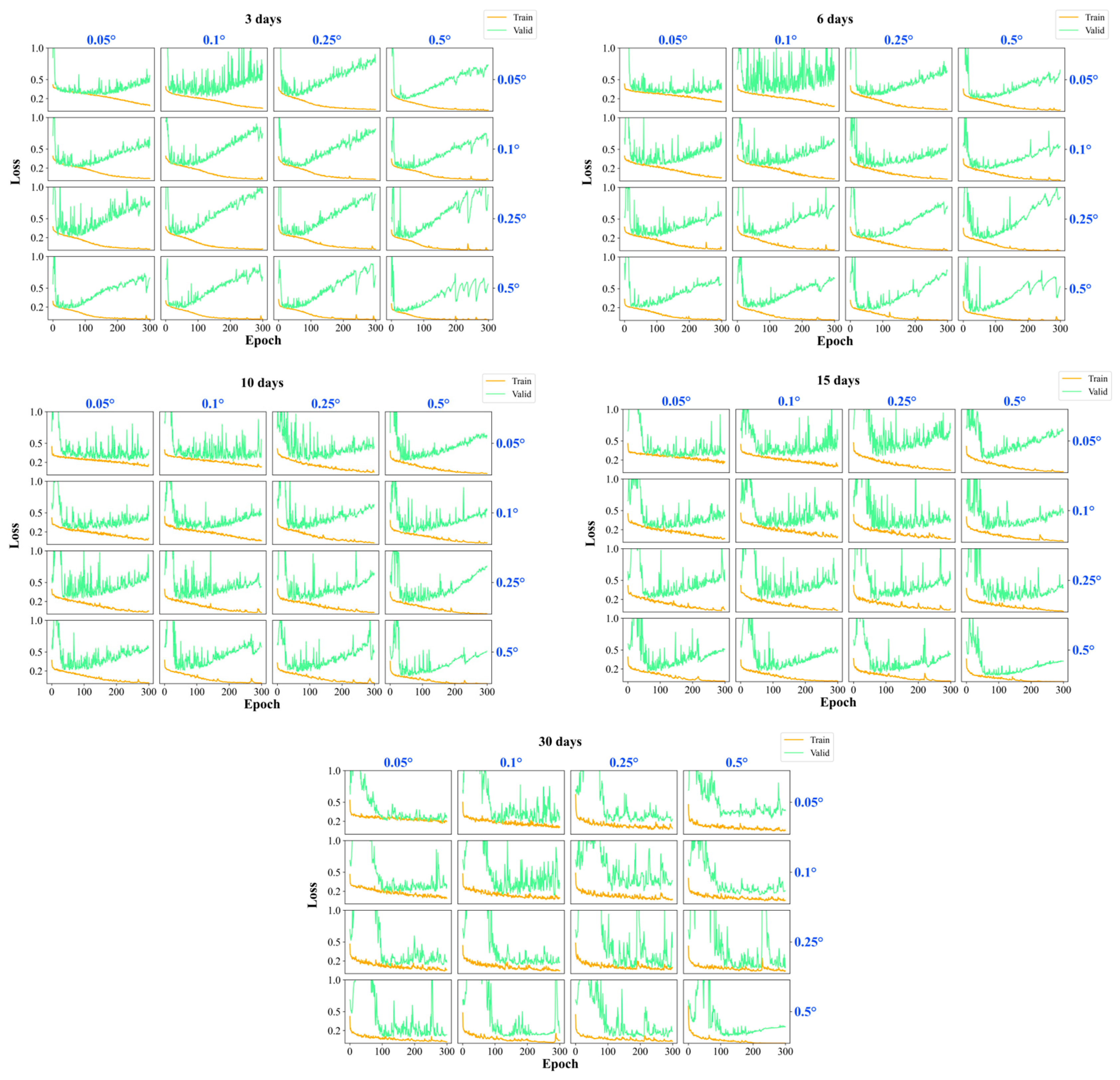
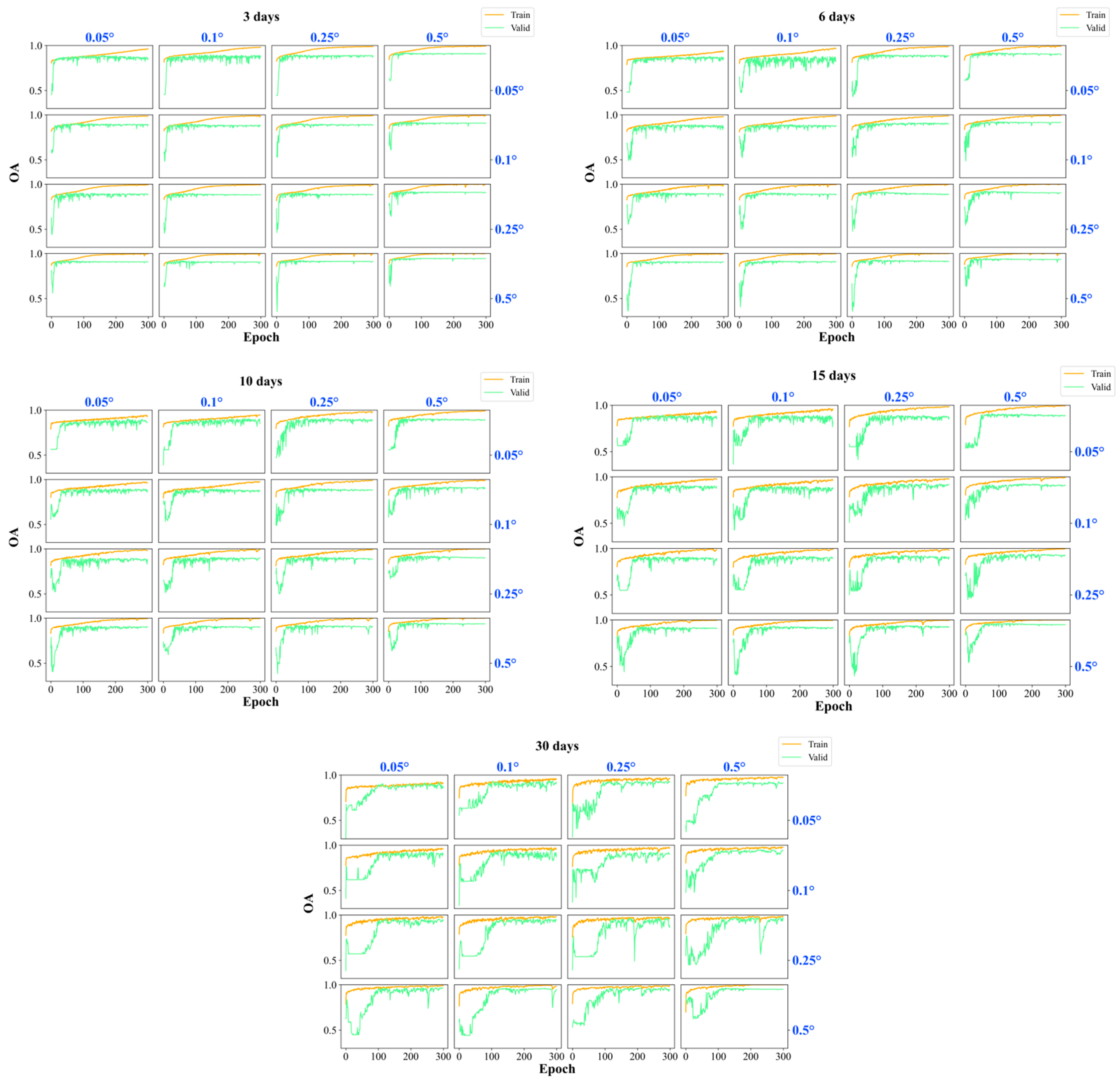
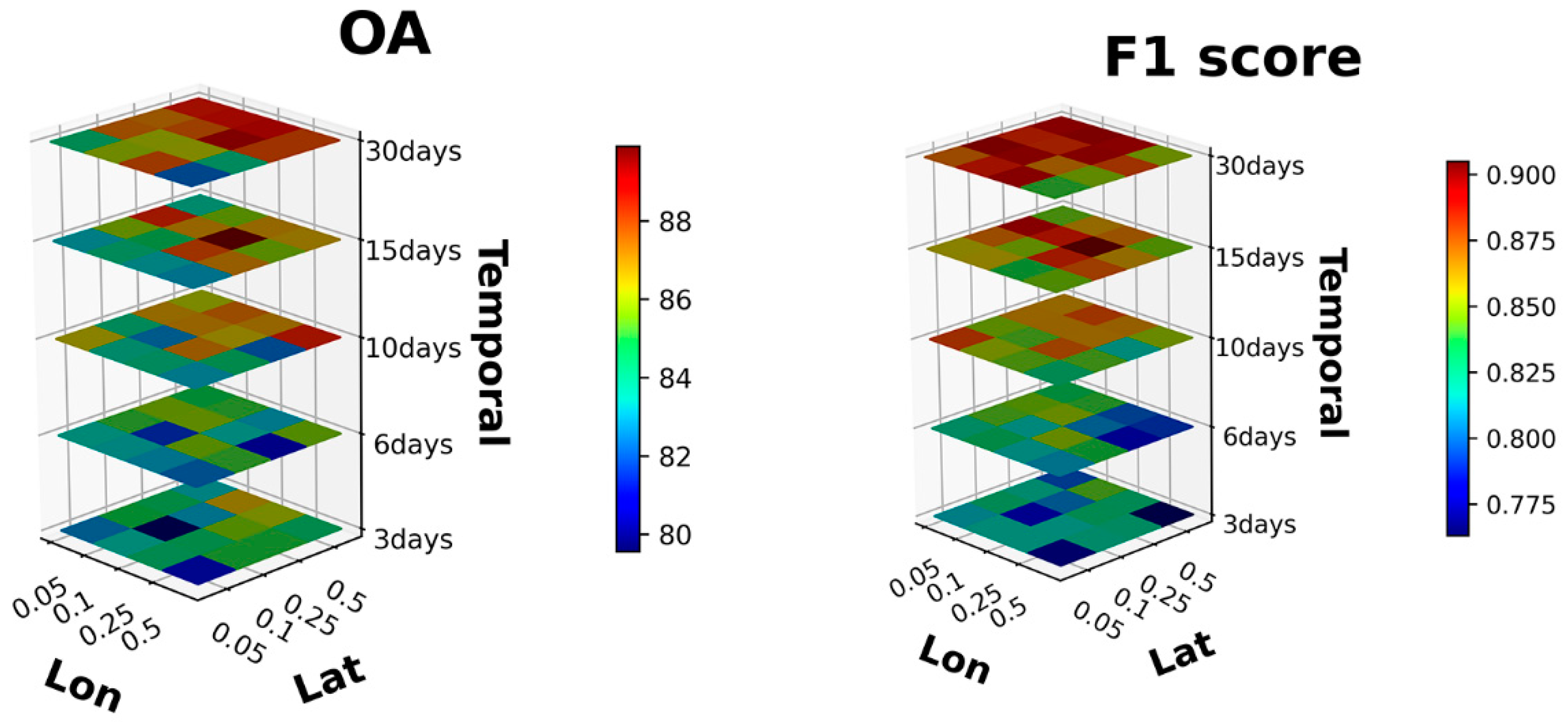
3.1. Model Results in Different Spatiotemporal Scales

In the different spatiotemporal scale cases, we obtained the following results. The minimum loss range for the training set is 0.03 to 0.25. For the validation set, the minimum loss range is 0.08 to 0.27, with an average of 0.19 (Figure 4). The optimal accuracy range for the validation set is 86.94% to 97.01%, with an average of 91.82% (Figure 5). An epoch refers to one complete pass through the entire training dataset during the training of a neural network. The loss curves of the training and validation sets reveal that all model cases, across different temporal and spatial scenarios, achieved a satisfactory fit within the 300-epoch limit. Additionally, the inclusion of two layers of SpatialDropout2D regularization helped mitigate model overfitting.

3.2. Spatiotemporal Scale Variability Evaluation

To assess the performance of the fishing ground prediction model under different temporal and spatial scales, it was tested on the testing set using OA and F1 score as evaluation metrics. The best performing case, with a spatial scale of 0.25° × 0.25° and a temporal scale of 15 days, achieved an OA of 89.90% and an F1 score of 0.9050, whereas the worst performing case, with a spatial scale of 0.1° × 0.1° and a temporal scale of 3 days, attained an OA of 79.56% and an F1 score of 0.7789. On average, the OA was 85.21% with a standard deviation of 2.12%, while the average F1 score was 0.8460 with a standard deviation of 0.03. Although the evaluation results varied, the overall performance was satisfactory (Figure 6). The findings indicated that a larger temporal scale leads to relatively better model performance. The influence of latitude in the spatial scale is more pronounced compared to longitude.

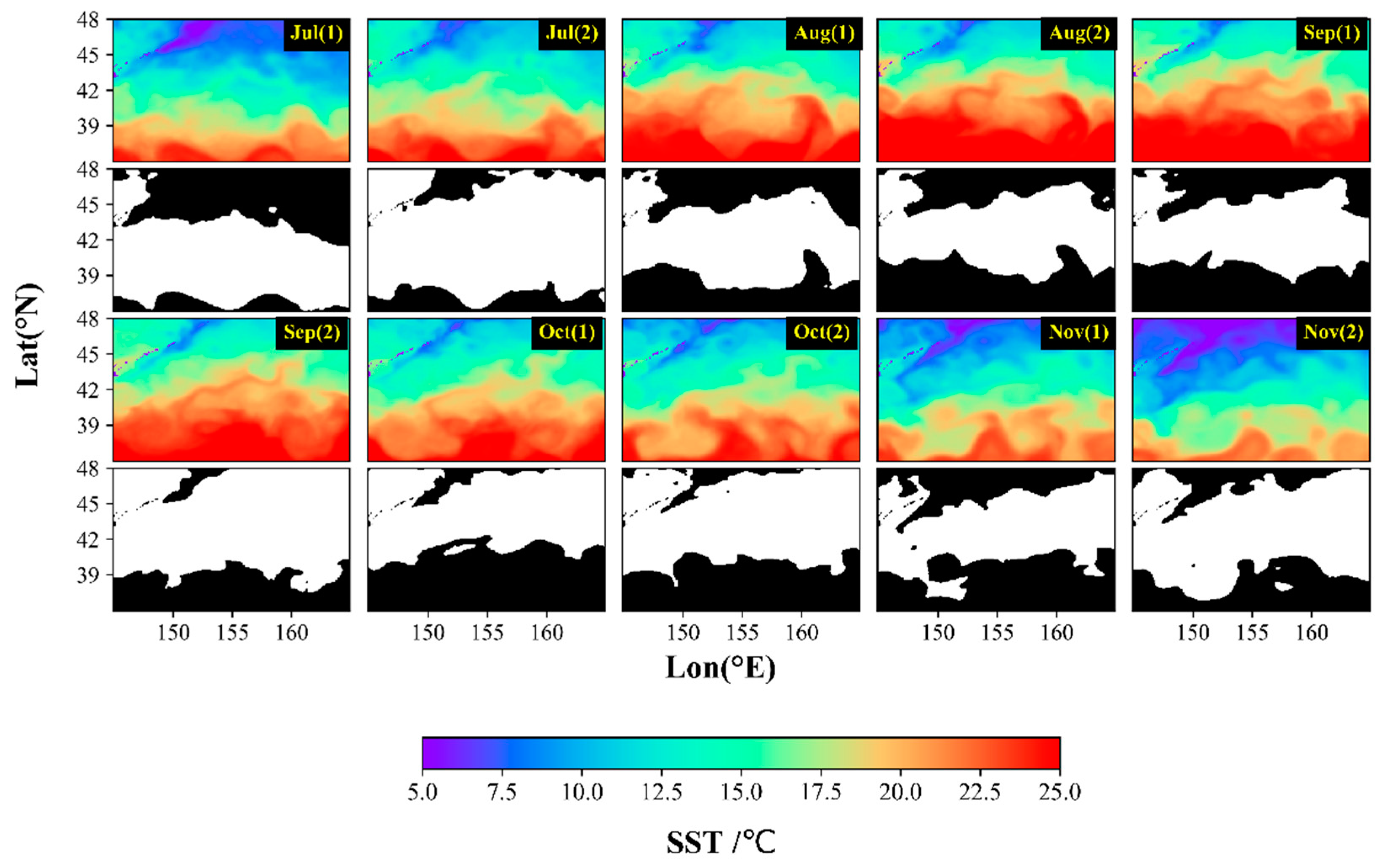
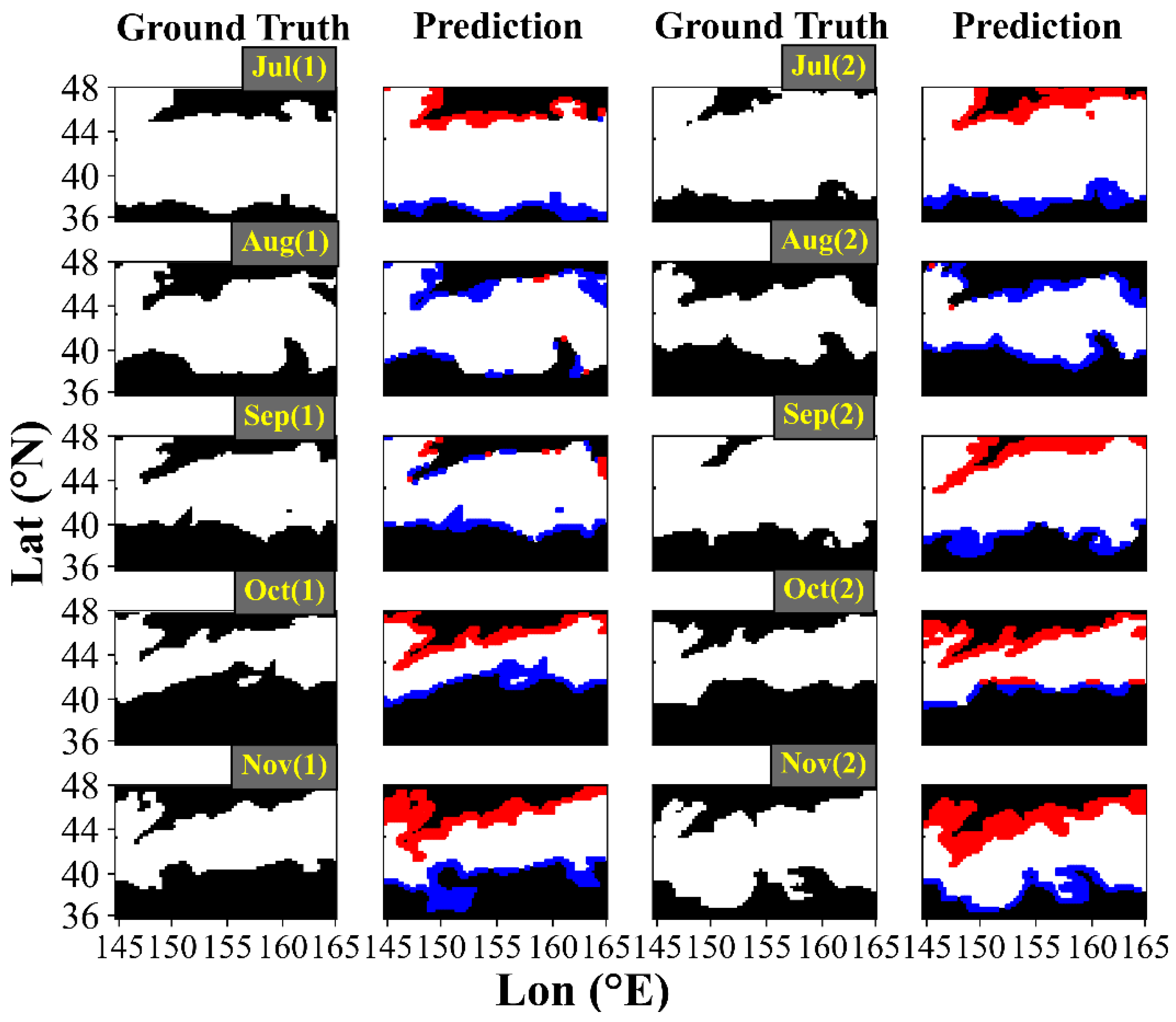
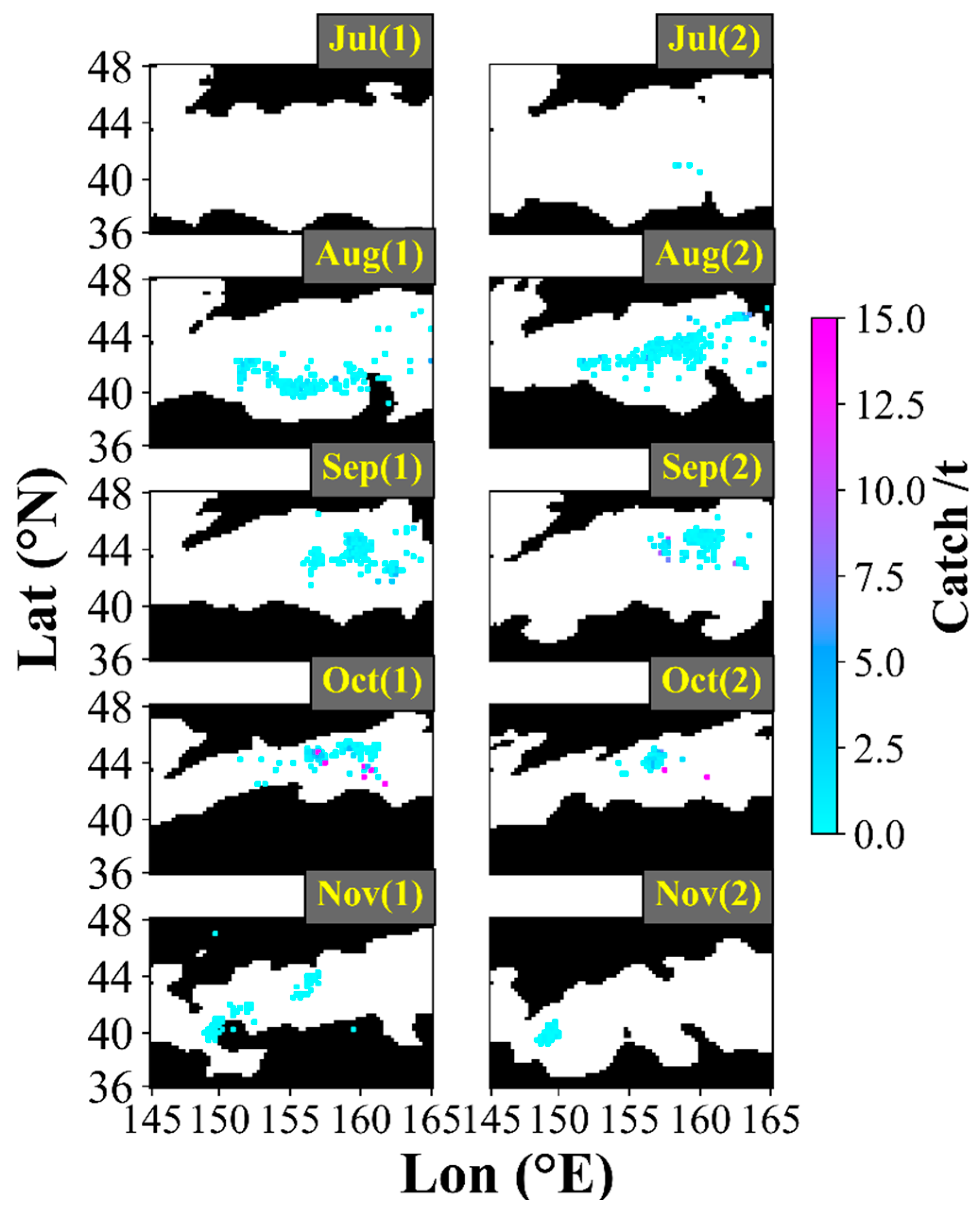
3.3. Prediction Performance of the Best Case

The best prediction performance was achieved in the first half of September, with an OA of 95.60% and an F1 score of 0.9600 (

Table 1. The testing results of the fishing ground prediction model in the best spatiotemporal scale case in each period.

Period	Overall Accuracy(OA, %)	Precision	Recall	F1 Score
July (1st half)	91.72	0.9427	0.9441	0.9434
July (2nd half)	88.75	0.9322	0.9160	0.9240
August (1st half)	94.51	0.9183	0.9974	0.9562
August (2nd half)	93.80	0.8810	0.9990	0.9360
September (1st half)	95.60	0.9390	0.9830	0.9600
September (2nd half)	87.55	0.9280	0.8910	0.9090
October (1st half)	90.55	0.8920	0.8610	0.8760
October (2nd half)	90.83	0.9229	0.8563	0.8883
November (1st half)	83.57	0.8553	0.7884	0.8205
November (2nd half)	82.14	0.9130	0.7701	0.8355
Mean ± Standard deviation	89.90 ± 4.25	0.9125 ± 0.0265	0.9005 ± 0.0782	0.9050 ± 0.0465

). During this period, the outline of the center fishing ground appeared smooth, and the prediction accuracy of the center fishing ground along the edge of the SST front at 44° to 48° N was high (Figure 7). Conversely, the worst prediction performance occurred in the second half of November, with an OA of 82.14% and an F1 score of 0.8355 (Table 1). In this period, the outline of the center fishing ground appeared relatively rough, and the correct prediction of the center fishing ground to the north of 44° N was challenging, particularly in the area of 145° to 150° E and 42° to 46° N. Overall, apart from November, the testing results for each period were satisfactory, confirming the model’s high stability over different periods. The fishing ground prediction model successfully extracted and predicted two significant pieces of information (Figure 7): the contour of the center fishing ground and the latitudinal change at different periods. However, the prediction results in November were not as accurate. The predicted center fishing grounds exhibited smoother outlines than the ground truth, and certain fine structures were not well predicted [36]. Furthermore, the prediction showed a southward shift compared to the ground truth, with higher SST values, which constituted the primary source of error.

4. Discussion

4.1. Impact of Asymmetric Spatiotemporal Scales on the Model

By examining the performance of models under various asymmetric spatial and temporal scale cases (Figure 6), significant differences in model performance are evident. Regarding temporal scales, the trends in OA and F1 are generally consistent. A larger temporal scale corresponds to better model performance (Figure 8). Concerning spatial scales, the influence of longitude and latitude on model performance is asymmetric. Cases with a longitude of 0.5° and a latitude of 0.05° are unfavorable for model results. When examining the dispersion across different spatial scales, it is observed that model performance exhibits greater dispersion in the latitude direction. This could be attributed to the fact that center fishing grounds are defined based on SST ranges, and changes in the latitude direction are more pronounced than in the longitude direction. Models with longitudes of 0.05° and 0.1° display more outliers in terms of dispersion. This could be due to the irregular distribution of center fishing grounds in the longitude direction, which does not conform to a normal distribution (Figure 8). Since both temporal and asymmetric spatial scales jointly influence model performance, the optimal case is determined to be 15 days for the temporal scale and 0.25° × 0.25° for the spatial scale. Previous studies have suggested optimal spatial scales ranging from 0.25° to 0.5° [25] and optimal temporal resolutions of 30 days [37]. The slight disparities between our results and previous research can be attributed to differences in data sources and models, along with the finding that a latitude of 0.5° yields better results, whereas a longitude of 0.5° yields poorer results in our study. Therefore, the previously established conclusion of a 0.5° optimal spatial scale might be influenced by the greater contribution of the latitude direction to model performance. The design of asymmetric spatial scales can better identify the most reasonable design case and enhance our understanding of distinct environmental characteristics in different marine regions.

Although there are substantial differences among various cases, the overall OA remains above 78%. Compared to traditional methods, the model has shown improvements in both accuracy and stability [1]. We believe this is because deep learning is more adept at handling the spatiotemporal distribution of fishing grounds compared to traditional methods, as evidenced by the U-Net model’s strong adaptability in pixel-level image segmentation. While the optimal spatiotemporal scale identified in this study is specific to Ommastrephes bartramii in the Northwest Pacific, other pelagic species may have different requirements for spatiotemporal scale (e.g., a minimum spatial scale of 0.5° for tuna [5]). However, the method proposed in this study does not rely on information specific to Ommastrephes bartramii. In other words, the concept of asymmetric spatiotemporal scale design presented in this paper can be extended to other species and may reveal different patterns of change in latitude, longitude, and temporal scales.

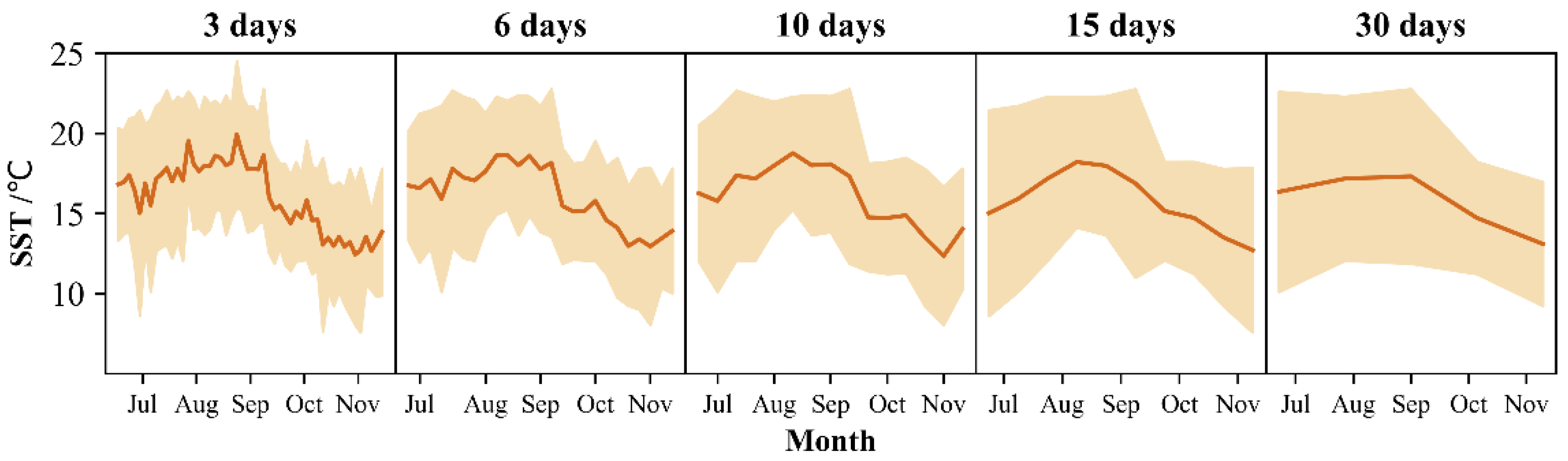
4.2. Impact of SST at Different Spatiotemporal Scales

SST is the most critical oceanic environmental factor affecting the distribution of pelagic commercial species [38,39,40,41,42]. The suitable SST range for Ommastrephes bartramii exhibits clear seasonal variation [1], characterized by an initial increase followed by a decrease, with the highest SST temperatures occurring in August and September. Examining the changes in the SST range of the center fishing grounds at different temporal scales (Figure 9), it becomes evident that with larger temporal scales, the SST range fluctuations of the center fishing grounds become smoother. This may lead to a better coupling between the environmental field and the center fishing grounds during model training, resulting in improved model performance. From a machine learning perspective, smaller temporal scales may offer a larger dataset for more comprehensive model training. However, from a fishery standpoint, the degree of matching between the environmental field and the fishing grounds also determines the model’s results.

Because the center fishing grounds are delineated based on the SST range, the distribution of center fishing grounds primarily exhibits a zonal pattern in the latitude direction. This results in a more pronounced impact of latitude on the model compared to longitude (Figure 10). The fishing ground of Ommastrephes bartramii is dominated by two western boundary currents, the Kuroshio Current characterized as a warm and nutrient-poor current and the Oyashio Current characterized as a cold and nutrient-rich current. The Kuroshio–Oyashio transition zone with high biological productivity is an important feeding ground for many commercially important marine species including Ommastrephes bartramii [43,44]. Due to the influence of the Kuroshio Current, the Oyashio Current, and their associated eddies on the longitudinal distribution of SST in the center fishing grounds [45], the model results are affected. In the study results, the adverse impact of the 0.5° longitude cases on the model outcomes may be attributed to the significant spacing between longitudes, which could lead to the neglect of oceanographic features, especially currents and eddies. On the other hand, the unfavorable effect of the 0.05° latitude cases on the model results could be due to the excessively small latitude scale, resulting in less noticeable variations in SST that fail to align well with the latitudinal changes in the center fishing grounds.

4.3. Application Evaluation of the Optimal Model

The U-Net model is widely recognized as one of the standard benchmarking methods for deep learning-based pixel-level image classification. Its defining feature is a fully convolutional structure, which eliminates the conventional fully connected layer and employs deconvolution layers to restore image resolution. This architectural choice significantly enhances the model’s training efficiency and accuracy when dealing with pixel-level image classification tasks. In other words, the deep learning model based on U-Net outperforms traditional convolutional models with fully connected layers in terms of suitability and efficiency, particularly in pixel-level fishing ground prediction [46].

In this study, actual catch data were used for model testing. The fishing grounds predicted by the model with optimal temporal and spatial scales on the 2020 testing dataset were compared with the actual catch data (Figure 11). Two metrics were employed to evaluate the model’s performance. First, the site coverage rate is defined as the ratio of the number of catch sites in fishing ground covered by the predicted fishing ground to the total catch sites. Second, the catch coverage rate is defined as the ratio of the catch value at the sites covered by the predicted fishing ground to the total catch value. The results (

Table 2. Application evaluation of the center fishing ground prediction model on the testing set with actual catch data.

Period	Site Coverage Rate (%)	Catch Coverage Rate (%)
July (1st half)	/	/
July (2nd half)	100.00	100.00
August (1st half)	98.57	99.81
August (2nd half)	99.68	99.95
September (1st half)	100.00	100.00
September (2nd half)	100.00	100.00
October (1st half)	100.00	100.00
October (2nd half)	100.00	100.00
November (1st half)	94.38	93.62
November (2nd half)	100.00	100.00

) showed that in the prediction, the site coverage rate for the first half of August is 98.57%, and the catch coverage rate is 99.81%; for the second half of August, the site coverage rate is 99.68%, and the catch coverage rate is 99.95%; and for the first half of November, the site coverage rate is 94.38%, and the catch coverage rate is 93.62%. Except for these three periods and the first half of July where no actual catch data are available, the site coverage rate and catch coverage rate for the other periods are 100%, indicating excellent application performance. Particularly in the first half of October, this period exhibits more sites with high catch values compared to other periods. Although the predicted center fishing ground during this period is relatively narrow, the application performance remains excellent, demonstrating the model’s robustness and reliability. Compared to the predicted fishing ground distribution in traditional methods, deep learning places greater emphasis on the application effectiveness of the test set in predicting results. This better reflects the deep learning approach’s ability to learn the mechanisms of fishing ground changes, and the model exhibits greater stability.

The impressive application performance of the deep learning-based model can be attributed to the following main reasons. (1) The definition of the center fishing ground based on the upper quartile effectively encompasses actual catch sites, even those with lower catch values. This method of defining the center fishing ground, tailored to the data characteristics of fishing grounds, is not only feasible but also reliable. It facilitates the successful application of deep learning to fishing ground prediction. (2) The U-Net model possesses distinctive characteristics within its convolutional layers, including weight sharing and local connectivity. These features help reduce the complexity of the image feature extraction network. The U-Net model strikes a delicate balance between extracting deep features for semantic classification and preserving high resolution. Consequently, it excels in handling pixel-level image classification tasks, enabling it to fully exploit the multiscale information embedded in SST data. This results in accurate and reliable pixel-level fishing ground predictions. Moreover, the SST distribution map and the center fishing ground map exhibit varying scales of features, such as the large-scale spatial distribution of the center fishing ground, the fine-scale bending of isotherms at the edges, and north–south shifts in the center fishing ground. The U-Net model effectively extracts and captures these features. This study provides a scientific basis for the high-quality development of distant-sea fisheries and the accurate predicting of fishing ground. It also offers technological support for the sustainable development of fishery resources in the Northwest Pacific.

However, this study still has some limitations. (1) Fishing ground changes are influenced not only by environmental factors such as SST but also by other anthropogenic factors, including the captain’s experience, decisions made by fishing enterprises, and the fishing equipment on the vessels. These factors will be taken into consideration in subsequent research. (2) Only one influencing factor, SST, was selected as the input factor, which may result in an excessively large area for the center fishing ground. Subsequent research will incorporate multiple factors and analyze the impact of asymmetric spatiotemporal scales on the model under the combination of multiple environmental factors.

5. Conclusions

In this study, we proposed an innovative deep learning-based approach for predicting fishing ground using asymmetric spatiotemporal scales, contributing to the refinement of existing research on this topic. The research lays the groundwork for the development of precise and stable models tailored to the specific spatiotemporal scales of a particular marine species within a defined region.

Through an analysis of results obtained from various combinations of temporal and asymmetric spatial scale cases, we found the optimal model parameters: a temporal scale of 15 days and a spatial scale of 0.25° × 0.25°. Larger temporal scales were found to enhance model accuracy, with latitude exerting a greater impact than longitude, likely influenced by the specific oceanographic characteristics of the Northwest Pacific.

The asymmetric spatiotemporal scale analysis deepens our understanding of how environmental factors influence fishing ground distribution. It is important to note that this study considered only SST as an influencing factor, and future research will explore the impact of integrating multiple environmental factors. The methods and insights presented, although specific to the Ommastrephes bartramii fishing ground, can be extended and applied to research involving fishing grounds of other species.

References

1. Chen, X. Theory and Method of Fisheries Forecasting; Springer Nature: Singapore, 2022. [Google Scholar]
2. Barash, A.; Scheinin, A.; Bigal, E.; Zemah Shamir, Z.; Martinez, S.; Davidi, A.; Fadida, Y.; Pickholtz, R.; Tchernov, D. Some Like It Hot: Investigating Thermoregulatory Behavior of Carcharhinid Sharks in a Natural Environment with Artificially Elevated Temperatures. Fishes 2023, 8, 428. [Google Scholar] [CrossRef]
3. Alioravainen, N.; Orell, P.; Erkinaro, J. Long-Term Trends in Freshwater and Marine Growth Patterns in Three Sub-Arctic Atlantic Salmon Populations. Fishes 2023, 8, 441. [Google Scholar] [CrossRef]
4. Free, C.M.; Thorson, J.T.; Pinsky, M.L.; Oken, K.L.; Wiedenmann, J.; Jensen, O.P. Impacts of historical warming on marine fisheries production. Science 2019, 363, 979–983. [Google Scholar] [CrossRef] [PubMed]
5. Zhang, T.; Song, L.; Yuan, H.; Song, B.; Ebango Ngando, N. A comparative study on habitat models for adult bigeye tuna in the Indian Ocean based on gridded tuna longline fishery data. Fish. Oceanogr. 2021, 30, 584–607. [Google Scholar] [CrossRef]
6. Fei, Y.; Yang, S.; Huang, M.; Wu, X.; Yang, Z.; Zhao, J.; Tang, F.; Fan, W.; Yuan, S. Evaluating Suitability of Fishing Areas for Squid-Jigging Vessels in the Northwest Pacific Ocean Derived from AIS Data. Fishes 2023, 8, 530. [Google Scholar] [CrossRef]
7. Li, G.; Xiong, Y.; Zhong, X.; Song, D.; Kang, Z.; Li, D.; Yang, F.; Wu, X. Characterizing Fishing Behaviors and Intensity of Vessels Based on BeiDou VMS Data: A Case Study of TACs Project for Acetes chinensis in the Yellow Sea. Sustainability 2022, 14, 7588. [Google Scholar] [CrossRef]
8. Sheaves, M.; Bradley, M.; Herrera, C.; Mattone, C.; Lennard, C.; Sheaves, J.; Konovalov, D.A. Optimizing video sampling for juvenile fish surveys: Using deep learning and evaluation of assumptions to produce critical fisheries parameters. Fish Fish. 2020, 21, 1259–1276. [Google Scholar] [CrossRef]
9. Reichstein, M.; Camps-Valls, G.; Stevens, B.; Jung, M.; Denzler, J.; Carvalhais, N.; Prabhat, F. Deep learning and process understanding for data-driven Earth system science. Nature 2019, 566, 195–204. [Google Scholar] [CrossRef] [PubMed]
10. Iqbal, U.; Li, D.; Akhter, M. Intelligent diagnosis of fish behavior using deep learning method. Fishes 2022, 7, 201. [Google Scholar] [CrossRef]
11. Ordoñez, A.; Eikvil, L.; Salberg, A.B.; Harbitz, A.; Elvarsson, B.Þ. Automatic fish age determination across different otolith image labs using domain adaptation. Fishes 2022, 7, 71. [Google Scholar] [CrossRef]
12. Kroodsma, D.A.; Mayorga, J.; Hochberg, T.; Miller, N.A.; Boerder, K.; Ferretti, F.; Wilson, A.; Bergman, B.; White, T.D.; Block, B.A.; et al. Tracking the global footprint of fisheries. Science 2018, 359, 904–908. [Google Scholar] [CrossRef]
13. Li, X.; Liu, B.; Zheng, G.; Ren, Y.; Zhang, S.; Liu, Y.; Gao, L.; Liu, Y.; Zhang, B.; Wang, F. Deep-learning-based information mining from ocean remote-sensing imagery. Natl. Sci. Rev. 2020, 7, 1584–1605. [Google Scholar] [CrossRef] [PubMed]
14. Rubbens, P.; Brodie, S.; Cordier, T.; Destro Barcellos, D.; Devos, P.; Fernandes-Salvador, J.A.; Fincham, J.I.; Gomes, A.; Handegard, N.O.; Howell, K.; et al. Machine learning in marine ecology: An overview of techniques and applications. ICES J. Mar. Sci. 2023, 80, 1829–1853. [Google Scholar] [CrossRef]
15. Liu, B.; Li, X.; Zheng, G. Coastal inundation mapping from bi-temporal and dual-polarization SAR imagery based on deep convolutional neural networks. J. Geophys. Res. 2019, 124, 9101–9113. [Google Scholar] [CrossRef]
16. Ham, Y.G.; Kim, J.H.; Luo, J.J. Deep learning for multi-year ENSO forecasts. Nature 2019, 573, 568–572. [Google Scholar] [CrossRef] [PubMed]
17. Landy, J.C.; Dawson, G.J.; Tsamados, M.; Bushuk, M.; Stroeve, J.C.; Howell, S.E.; Krumpen, T.; Babb, D.G.; Komarov, A.S.; Heorton, H.B.S.; et al. A year-round satellite sea-ice thickness record from CryoSat-2. Nature 2022, 609, 517–522. [Google Scholar] [CrossRef] [PubMed]
18. Nathan, R.; Monk, C.T.; Arlinghaus, R.; Adam, T.; Alós, J.; Assaf, M.; Baktoft, H.; Beardsworth, C.E.; Bertram, M.G.; Bijleveld, A.I.; et al. Big-data approaches lead to an increased understanding of the ecology of animal movement. Science 2022, 375, eabg1780. [Google Scholar] [CrossRef] [PubMed]
19. Ouyang, J.; Liu, S.; Peng, H.; Garg, H.; Thanh, D.N. LEA U-Net: A U-Net-based deep learning framework with local feature enhancement and attention for retinal vessel segmentation. Complex Intell. Syst. 2023, 9, 6753–6766. [Google Scholar] [CrossRef]
20. Ronneberger, O.; Fischer, P.; Brox, T. U-net: Convolutional networks for biomedical image segmentation. In Proceedings of the International Conference on Medical Image Computing and Computer-Assisted Intervention, Munich, Germany, 5–9 October 2015; Springer International Publishing: Cham, Switzerland, 2015; pp. 234–241. [Google Scholar]
21. Xie, M.; Liu, B.; Chen, X. Prediction on fishing ground of Ommastrephes bartramii in Northwest Pacific based on deep learning. J. Fish. China 2022, 1–13. Online Publication. (In Chinese) [Google Scholar]
22. Chollett, I.; Perruso, L.; O’Farrell, S. Toward a better use of fisheries data in spatial planning. Fish Fish. 2022, 23, 1136–1149. [Google Scholar] [CrossRef]
23. Meng, W.; Gong, Y.; Wang, X.; Tong, J.; Han, D.; Chen, J.; Wu, J. Influence of spatial scale selection of environmental factors on the prediction of distribution of Coilia nasus in Changjiang River Estuary. Fishes 2021, 6, 48. [Google Scholar] [CrossRef]
24. Tian, S.; Chen, Y.; Chen, X.; Xu, L.; Dai, X. Impacts of spatial scales of fisheries and environmental data on catch per unit effort standardization. Mar. Freshw. Res. 2010, 60, 1273–1284. [Google Scholar] [CrossRef]
25. Feng, Y.; Cui, L.; Chen, X.; Chen, L.; Yang, Q. Impacts of changing spatial scales on CPUE-factor relationships of Ommastrephes bartramii in the northwest Pacific. Fish. Oceanogr. 2019, 28, 143–158. [Google Scholar] [CrossRef]
26. Ciannelli, L.; Fauchald, P.; Chan, K.S.; Agostini, V.N.; Dingsør, G.E. Spatial fisheries ecology: Recent progress and future prospects. J. Mar. Syst. 2008, 71, 223–236. [Google Scholar] [CrossRef]
27. Chagaris, D.; Mahmoudi, B.; Muller-Karger, F.; Cooper, W.; Fischer, K. Temporal and spatial availability of Atlantic Thread Herring, Opisthonema oglinum, in relation to oceanographic drivers and fishery landings on the Florida Panhandle. Fish. Oceanogr. 2015, 24, 257–273. [Google Scholar] [CrossRef]
28. Zhu, W.; Sun, W.; Li, D.; Han, L. Spatial-Temporal Characteristics and Influencing Factors of Marine Fishery Eco-Efficiency in China: Evidence from Coastal Regions. Fishes 2023, 8, 438. [Google Scholar] [CrossRef]
29. Guinet, C.; Dubroca, L.; Lea, M.A.; Goldsworthy, S.; Cherel, Y.; Duhamel, G.; Bonadonna, F.; Donnay, J.P. Spatial distribution of foraging in female Antarctic fur seals Arctocephalus gazella in relation to oceanographic variables: A scale-dependent approach using geographic information systems. Mar. Ecol. Prog. Ser. 2001, 219, 251–264. [Google Scholar] [CrossRef]
30. Forsythe, J.W. Accounting for the effect of temperature on squid growth in nature: From hypothesis to practice. Mar. Freshw. Res. 2004, 55, 331–339. [Google Scholar] [CrossRef]
31. Brander, K. Impacts of climate change on fisheries. J. Mar. Syst. 2010, 79, 389–402. [Google Scholar] [CrossRef]
32. Li, M.; Xu, Y.; Sun, M.; Li, J.; Zhou, X.; Chen, Z.; Zhang, K. Impacts of Strong ENSO Events on Fish Communities in an Overexploited Ecosystem in the South China Sea. Biology 2023, 12, 946. [Google Scholar] [CrossRef] [PubMed]
33. Tian, S.; Chen, X.; Chen, Y.; Xu, L.; Dai, X. Standardizing CPUE of Ommastrephes bartramii for Chinese squid-jigging fishery in Northwest Pacific Ocean. Chin. J. Oceanol. Limnol. 2009, 27, 729–739. [Google Scholar] [CrossRef]
34. Krizhevsky, A.; Sutskever, I.; Hinton, G.E. ImageNet classification with deep convolutional neural networks. Commun. ACM 2017, 60, 84–90. [Google Scholar] [CrossRef]
35. Tompson, J.; Goroshin, R.; Jain, A.; LeCun, Y.; Bregler, C. Efficient object localization using convolutional networks. In Proceedings of the IEEE Conference on Computer Vision and Pattern Recognition, Boston, MA, USA, 7–12 June 2015; pp. 648–656. [Google Scholar]
36. Ravuri, S.; Lenc, K.; Willson, M.; Kangin, D.; Lam, R.; Mirowski, P.; Fitzsimons, M.; Athanassiadou, M.; Kashem, S.; Madge, S.; et al. Skilful precipitation nowcasting using deep generative models of radar. Nature 2021, 597, 672–677. [Google Scholar] [CrossRef] [PubMed]
37. Gong, C.; Chen, X.; Gao, F.; Tian, S. Effect of spatial and temporal scales on habitat suitability modeling: A case study of Ommastrephes bartramii in the northwest Pacific Ocean. J. Ocean Univ. China 2014, 13, 1043–1053. [Google Scholar] [CrossRef]
38. Suca, J.J.; Santora, J.A.; Field, J.C.; Curtis, K.A.; Muhling, B.A.; Cimino, M.A.; Hazen, E.; Bograd, S.J. Temperature and upwelling dynamics drive market squid (Doryteuthis opalescens) distribution and abundance in the California Current. ICES J. Mar. Sci. 2022, 79, 2489–2509. [Google Scholar] [CrossRef]
39. Friedland, K.D.; Reddin, D.G.; McMenemy, J.R.; Drinkwater, K.F. Multidecadal trends in North American Atlantic salmon (Salmo salar) stocks and climate trends relevant to juvenile survival. Can. J. Fish. Aquat. Sci. 2023, 60, 563–583. [Google Scholar] [CrossRef]
40. Shi, Y.; Kang, B.; Fan, W.; Xu, L.; Zhang, S.; Cui, X.; Dai, Y. Spatio-Temporal Variations in the Potential Habitat Distribution of Pacific Sardine (Sardinops sagax) in the Northwest Pacific Ocean. Fishes 2023, 8, 86. [Google Scholar] [CrossRef]
41. Wiryawan, B.; Loneragan, N.; Mardhiah, U.; Kleinertz, S.; Wahyuningrum, P.I.; Pingkan, J.; Wildan; Timur, P.S.; Duggan, D.; Yulianto, I. Catch per unit effort dynamic of yellowfin tuna related to sea surface temperature and chlorophyll in Southern Indonesia. Fishes 2020, 5, 28. [Google Scholar] [CrossRef]
42. Mondal, S.; Vayghan, A.H.; Lee, M.; Wang, Y.; Semedi, B. Habitat suitability modeling for the feeding ground of immature Albacore in the Southern Indian Ocean using satellite-derived sea surface temperature and chlorophyll data. Remote Sens. 2021, 13, 2669. [Google Scholar] [CrossRef]
43. Ohshimo, S.; Hiraoka, Y.; Sato, T.; Nakatsuka, S. Feeding habits of bigeye tuna (Thunnus obesus) in the north pacific from 2011 to 2013. Mar. Freshw. Res. 2018, 69, 585–606. [Google Scholar] [CrossRef]
44. Ishak, N.H.A.; Tadokoro, K.; Okazaki, Y.; Kakehi, S.; Suyama, S.; Takahashi, K. Distribution, biomass, and species composition of salps and doliolids in the Oyashio-Kuroshio transitional region: Potential impact of massive bloom on the pelagic food web. J. Oceanogr. 2020, 76, 351–363. [Google Scholar] [CrossRef]
45. Zhang, Y.; Yu, W.; Chen, X.; Zhou, M.; Zhang, C. Evaluating the impacts of mesoscale eddies on abundance and distribution of neon flying squid in the Northwest Pacific Ocean. Front. Mar. Sci. 2022, 9, 862273. [Google Scholar] [CrossRef]
46. Han, H.; Jiang, B.; Shi, Y.; Jiang, P.; Zhang, H.; Shang, C.; Sun, Y.; Li, Y.; Xiang, D. Response of the Northwest Indian Ocean purpleback flying squid (Sthenoteuthis oualaniensis) fishing grounds to marine environmental changes and its prediction model construction based on multi-models and multi-spatial and temporal scales. Ecol. Indic. 2023, 154, 110809. [Google Scholar] [CrossRef]
Figure 1. Distribution of Ommastrephes bartramii fishing ground in the Northwest Pacific Ocean.
Fishes 09 00064 g001
Figure 2. Case design of different asymmetric temporal and spatial scales.
Fishes 09 00064 g002
Figure 3. Architecture of the fishing ground prediction model Examples are a spatial scale of 0.05° × 0.05° and a temporal scale of 3 days. In the figure, conv stands for convolution, and ReLU stands for the rectified linear unit.
Fishes 09 00064 g003
Figure 4. Loss curves of the training and validation sets of the fishing ground prediction model in different temporal and spatial scales. Train and Valid in the figure represent the training and validation sets, respectively.
Fishes 09 00064 g004
Figure 5. Overall accuracy curves of the training and validation set of the fishing ground prediction model in different temporal and spatial scales. In the figure, OA stands for overall accuracy, and Train and Valid stand for the training and validation set, respectively.
Fishes 09 00064 g005
Figure 6. Performance evaluation on the testing set of the fishing ground prediction model in different temporal scales.
Fishes 09 00064 g006
Figure 7. Visual evaluation of the performance of the center fishing ground model in the best case. Jul (1), Jul (2), …, and Nov (2) represent the first half of July, the second half of July, …, and the second half of November, respectively. In the ground truth, the center fishing ground and non-center fishing ground are shown in white and black, respectively. In the prediction, the correctly predicted center fishing ground and non-center fishing ground are shown in white and black, respectively; the falsely predicted center fishing ground and non-center fishing ground are shown in blue and red, respectively.
Fishes 09 00064 g007
Figure 8. Dispersion and trend of model performance at different temporal and spatial scales (longitude and latitude).
Fishes 09 00064 g008
Figure 9. Variation in the sea surface temperature (SST) range in the center fishing ground of Ommastrephes bartramii in different temporal scale cases (an example is a spatial scale of 0.05° × 0.05°).
Fishes 09 00064 g009
Figure 10. Temporal changes in SST and the corresponding center fishing grounds.
Fishes 09 00064 g010
Figure 11. Actual catch data superimposed onto the predicted results (the predicted center fishing ground is illustrated in white, the predicted non-center fishing ground in black, and the actual catch data as colored dots.).
Fishes 09 00064 g011