Spatiotemporal Variations and Convergence Characteristics of Green Technological Progress in China’s Mariculture

Abstract

The sustainability of mariculture depends on adopting green technologies, which can mitigate the negative impacts on the environment and ensure long-term viability. However, existing studies do not comprehensively understand the characteristics and regional differences of green technology progress (GTP) in mariculture. According to data from ten coastal regions from 2008 to 2020, this study adopts the Epsilon-Based Measure (EBM)-Malmquist model to measure the GTP of mariculture, uses the Dagum Gini coefficient to analyze the spatial differences of GTP, and uses convergence models to explore the convergence of GTP. The results showed that: (1) the GTP of China’s mariculture showed a fluctuating upward trend temporally and significant spatial differences. The overall differences showed a dispersion trend over time. The contributions of inter-regional super variable net value difference (Gnb), inter-regional transvariation intensity (Gt), and intra-regional difference (Gw) were 38.813%, 31.256%, and 29.931%, respectively. (2) The degree of dispersion of GTP among different regions has not decreased with time, which means there is no apparent σ convergence. Absolute β convergence and conditional β convergence existed in GTP, and the absolute value of the latter was greater than that of the former. That is, the growth rate of GTP will first reach their respective steady-state levels and then approach a unified steady-state equilibrium level.

1. Introduction

Food security has always been one of the core issues of global focus [1]. Along with the continuous modernization process in China, the per capita income level has been increasing, accelerating the consumption structure’s upgrading. Together with the impact of the continuous growth of the total population, the demand for food continuously increases [2]. However, China’s cultivated land and fishery resources are decreasing. Therefore, constructing a “blue granary” and vigorously developing mariculture is key to solving China’s food security problems [3]. As the development of the marine aquaculture industry is still dominated by extensive production methods, the problems of aquaculture pollution in China’s offshore waters are becoming increasingly severe, threatening its sustainability [4,5,6]. The 14th Five-Year Plan for National Fisheries Development clearly instructs to “promote green and healthy aquaculture, stable the production and supply level of aquatic products,” which requires coastal regions to improve the green total factor productivity (GTFP) of mariculture and promote its healthy development [7]. The GTFP of mariculture includes the influence of green technology progress (GTP) and green technology efficiency (GTE). It has been found that improvement in the GTFP of mariculture is mainly due to GTP [8,9]. Therefore, promoting GTP in the mariculture industry will lead to the rapid development of China’s marine economy. However, due to regional differences in economic development levels and characteristics, there is a significant difference in the GTP level of mariculture between regions [10]. Therefore, it is of great practical significance to study the spatial and temporal characteristics of mariculture GTP, whether the degree of dispersion and the gaps in GTP in mariculture between regions will gradually decrease, and whether the convergence rate will change.

With the increasingly significant role of mariculture in promoting the development of the marine economy, technological progress (TP) in mariculture has gradually attracted widespread attention. Sun and Ji (2022) [11] decomposed the Malmquist index based on the data envelopment analysis (DEA) to measure input-biased TP in mariculture and explore its contribution to total factor productivity (TFP). Furthermore, Ji et al. (2022) [12] analyzed the green output bias of mariculture TP by identifying the bias of TP among output factors in conjunction with the changes in marginal factor substitution rates over time. The study shows that TP profoundly impacts the development of mariculture in China. However, with the rapid development of mariculture, the severe damage to the marine ecological environment attracted people’s attention [13,14,15,16,17,18]. Several scholars considered the environment in mariculture research, but most have focused on the effects of GTP on GTFP. For example, considering environmental constraints, Guo et al. (2022) [9] used the SBM-ML model to decompose the TFP of aquaculture into GTP and GTE to explore the variation of GTFP in mariculture and freshwater aquaculture. Ji and Zeng (2017) [10] and Ji and Li (2019) [19] used the Global ML model and the EBM-Global ML model to measure GTFP in detail. The results show that the improvement of GTFP in Chinese mariculture was mainly due to TP. Ren and Zeng (2021) [20] confirmed the effect of GTP on the improvement of mariculture productivity and studied the direction of green-biased technological progress. The above studies help to clarify the crucial mechanisms of GTFP enhancement, but it is challenging to identify the determinants of changes in TP.

Overall, some studies have specifically addressed the GTP in mariculture, but academic papers on its spatiotemporal variation and convergence characteristics are almost non-existent. This study aims to fill this gap. Therefore, this study used the EBM-Malmquist method to calculate the GTP of China’s mariculture reasonably and further analyzed the convergence of GTP in the mariculture industry in China as a whole and among different regions. In addition, this study conducts an in-depth analysis of the forms of convergence of GTP in mariculture among different regions.

2. Materials and Methods

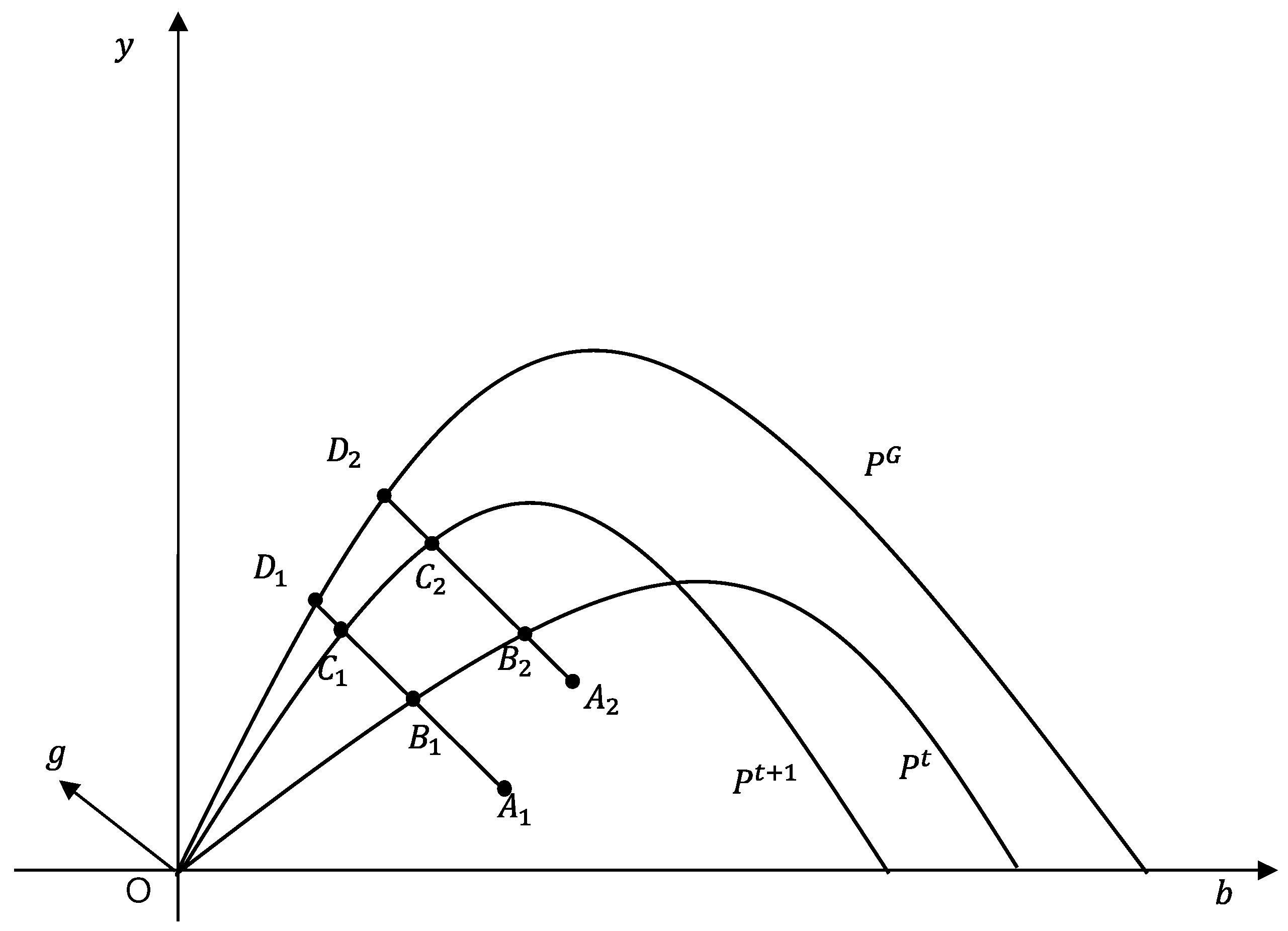
2.1. Method for Measuring GTP in Mariculture

This study uses the EBM method proposed by Tone and Tsutsui (2010) [21] to measure the GTP of China’s mariculture. The EBM method can avoid the model setting deviation caused by a preset production function between input and output, which can guarantee the validity of research results to a great extent. Furthermore, the EBM model is based on a mixed distance function, so it combines the advantages of the radial distance function (the Charnes, Cooper, and Rhodes model and the Banker, Charnes, and Cooper model) and non-radial distance function (the slack-based measure model) in the traditional DEA model [22]. Therefore, using the EBM model can improve the accuracy of the measurement to a great extent. The EBM model construction in this study is shown in Formulas (1)–(5).

$$\mathsf{\gamma }=\mathrm{m}\mathrm{i}\mathrm{n}\frac{\mathsf{\theta }-{\mathsf{\epsilon }}_{\mathrm{x}}\sum _{\mathrm{i}=1}^{\mathrm{m}}\frac{{\mathsf{\omega }}_{\mathrm{i}}^{-}{\mathrm{s}}_{\mathrm{i}}^{-}}{{\mathrm{x}}_{\mathrm{i}\mathrm{k}}}}{\mathsf{\phi }+{\mathsf{\epsilon }}_{\mathrm{y}}\sum _{\mathrm{j}=1}^{\mathrm{s}}\frac{{\mathsf{\omega }}_{\mathrm{j}}^{+}{\mathrm{s}}_{\mathrm{j}}^{+}}{{\mathrm{y}}_{\mathrm{j}\mathrm{k}}}+{\mathsf{\epsilon }}_{\mathrm{b}}\sum _{\mathrm{z}=1}^{\mathrm{l}}\frac{{\mathsf{\omega }}_{\mathrm{z}}^{-}{\mathrm{s}}_{\mathrm{z}}^{-}}{{\mathrm{b}}_{\mathrm{z}\mathrm{k}}}}$$

(1)

$$\mathrm{s}.\mathrm{t}. \mathrm{X}\mathsf{\delta }+{\mathrm{s}}_{\mathrm{i}}^{-}=\mathsf{\theta }\mathrm{x},\mathrm{i}=\mathrm{1,2},\cdots ,\mathrm{m}$$

(2)

$$\mathrm{Y}\mathsf{\delta }-{\mathrm{s}}_{\mathrm{j}}^{+}=\mathsf{\phi }\mathrm{y},\mathrm{j}=\mathrm{1,2},\cdots ,\mathrm{s}$$

(3)

$$\mathrm{B}\mathsf{\delta }+{\mathrm{s}}_{\mathrm{z}}^{-}=\mathsf{\phi }\mathrm{b},\mathrm{z}=\mathrm{1,2},\cdots ,\mathrm{l}$$

(4)

$$\mathsf{\delta }\ge 0,{\mathrm{s}}_{\mathrm{i}}^{-},{\mathrm{s}}_{\mathrm{j}}^{+},{\mathrm{s}}_{\mathrm{z}}^{-}\ge 0$$

(5)

where $\mathsf{\gamma }$ represents the target efficiency value. This study refers to the GTFP of mariculture, the value of which is in the range [0, 1]. $\mathrm{x}$ represents the input variable; y represents the desirable output variable; b represents the undesirable output variable; and ω and s represent the weight and relaxation variable, respectively. $\mathsf{\epsilon }$ is a core parameter of the EBM model, an important indicator synthesizing the radial efficiency value θ and the non-radial slack variable. Its value range is [0, 1]. When $\mathsf{\epsilon }=0$, it is equivalent to the radial CCR model; when $\mathsf{\epsilon }=1$, it is equivalent to the SBM model. When $\mathsf{\epsilon }$ is between 0 and 1, it indicates that the model contains both radial and non-radial slack variable parts.

In order to obtain the GTP index of mariculture, it is necessary to decompose the calculated GTFP. This study uses Oh’s (2010) [23] Global Malmquist–Luenberger (GML) index constructed from the perspective of global production to decompose it. The GML index is obtained by optimizing the traditional Malmquist–Luenberger (ML) index, which can effectively avoid the disadvantages of linear programming without solutions that may occur in ML exponential decomposition [24].

Figure 1 shows the composition of the common frontier, which can reflect the principle of the GML index. The GML index analyzes changes in total factor productivity from a global perspective. The global frontier envelops the production possibility set for all periods:

$${\mathrm{P}}^{\mathrm{G}}={\mathrm{P}}^1\cup {\mathrm{P}}^2{\cup \mathrm{P}}^{\mathrm{T}}$$

${\mathrm{A}}_1$ and ${\mathrm{A}}_2$ are the production points in periods t and t + 1, respectively. ${\mathrm{B}}_1$, ${\mathrm{B}}_2$, ${\mathrm{C}}_1$, ${\mathrm{C}}_2$, ${\mathrm{D}}_1$, and ${\mathrm{D}}_2$ represent the distances of ${\mathrm{A}}_1$ and ${\mathrm{A}}_2$ to different frontiers. The GML index is no longer represented by the geometric mean of the two indices but by the distance between the production points of the two adjacent periods and the common frontier. It avoids the problem of arbitrary choices and also gives the model transferability. The specific formula is as follows:

$$\begin{array}{c}{\mathrm{G}\mathrm{M}\mathrm{L}}^{\mathrm{t},\mathrm{t}+1}\left({\mathrm{x}}^{\mathrm{t}},{\mathrm{y}}^{\mathrm{t}},{\mathrm{b}}^{\mathrm{t}},{\mathrm{x}}^{\mathrm{t}+1},{\mathrm{y}}^{\mathrm{t}+1},{\mathrm{b}}^{\mathrm{t}+1}\right)=\frac{{\mathrm{E}}^{\mathrm{G},\mathrm{t}+1}\left({\mathrm{x}}^{\mathrm{t}+1},{\mathrm{y}}^{\mathrm{t}+1},{\mathrm{b}}^{\mathrm{t}+1}\right)}{{\mathrm{E}}^{\mathrm{G},\mathrm{t}}\left({\mathrm{x}}^{\mathrm{t}},{\mathrm{y}}^{\mathrm{t}},{\mathrm{b}}^{\mathrm{t}}\right)}\\ \hspace{1em}\hspace{1em}\hspace{1em}\hspace{1em}\hspace{1em}\hspace{1em}\hspace{1em}=\frac{{\mathrm{E}}^{\mathrm{t}+1}\left({\mathrm{x}}^{\mathrm{t}+1},{\mathrm{y}}^{\mathrm{t}+1},{\mathrm{b}}^{\mathrm{t}+1}\right)}{{\mathrm{E}}^{\mathrm{t}}\left({\mathrm{x}}^{\mathrm{t}},{\mathrm{y}}^{\mathrm{t}},{\mathrm{b}}^{\mathrm{t}}\right)}\times \frac{{\mathrm{E}}^{\mathrm{G},\mathrm{t}+1}\left({\mathrm{x}}^{\mathrm{t}+1},{\mathrm{y}}^{\mathrm{t}+1},{\mathrm{b}}^{\mathrm{t}+1}\right)/{\mathrm{E}}^{\mathrm{t}+1}\left({\mathrm{x}}^{\mathrm{t}+1},{\mathrm{y}}^{\mathrm{t}+1},{\mathrm{b}}^{\mathrm{t}+1}\right)}{{\mathrm{E}}^{\mathrm{G},\mathrm{t}}\left({\mathrm{x}}^{\mathrm{t}},{\mathrm{y}}^{\mathrm{t}},{\mathrm{b}}^{\mathrm{t}}\right)/{\mathrm{E}}^{\mathrm{t}}\left({\mathrm{x}}^{\mathrm{t}},{\mathrm{y}}^{\mathrm{t}},{\mathrm{b}}^{\mathrm{t}}\right)}={\mathrm{G}\mathrm{T}\mathrm{E}}^{\mathrm{t},\mathrm{t}+1}\times {\mathrm{G}\mathrm{T}\mathrm{P}}^{\mathrm{t},\mathrm{t}+1}\end{array}$$

(6)

where $\mathrm{E}(\mathrm{G},\mathrm{t})$ represents the efficiency value of the $\mathrm{t}$ period from the perspective of global production, and GML represents the GTFP of mariculture, which is further decomposed to obtain the GTE and GTP in mariculture.

Using the data from 10 coastal provinces in China as the sample, including Liaoning, Tianjin, Hebei, Shandong, Jiangsu, Fujian, Zhejiang, Guangdong, Guangxi, and Hainan, and excluding Hong Kong, Macau, Taiwan, and Shanghai due to data availability, this study calculates GTP in China’s mariculture from 2008 to 2020. Estimating the GTP of mariculture requires defining the input and output variables. The input and output variables are selected referring to the existing research [14,25]. There are two output variables: (1) Gross output value of mariculture (Y). This study uses the gross output value of mariculture as the desirable output variable, which can accurately reflect the change in scale and benefits of mariculture development in China. (2) Equivalent pollution load (E). This is obtained by estimating the pollutants produced in the process of mariculture and converting the different types of pollutants into a standard intermediate mass, according to the Handbook of Discharge Coefficients of Pollution Sources in Aquaculture [26]. This study uses this as an undesirable output variable in mariculture. There are two input variables: (1) Mariculture area (M). This uses the scale of the mariculture area in 10 coastal provinces to measure the scale of Chinese mariculture. (2) Mariculture capital stock (C). The current statistical data in China lack direct information on the mariculture capital stock, so this study uses the perpetual inventory method to estimate the level of mariculture capital stock [27]. The formula is as follows:

$${\mathrm{C}}_{\mathrm{i},\mathrm{t}+1}={\mathrm{I}}_{\mathrm{i},\mathrm{t}+1}+\left(1-\mathsf{\delta }\right){\mathrm{C}}_{\mathrm{i},\mathrm{t}}$$

(7)

$${\mathrm{C}}_{\mathrm{i},\mathrm{t}}={\mathrm{I}}_{\mathrm{i},\mathrm{t}}/\left({\mathrm{g}}_{\mathrm{i},\mathrm{t}}+\mathsf{\delta }\right)$$

(8)

where ${\mathrm{C}}_{\mathrm{i},\mathrm{t}}$ is the capital stock of province $\mathrm{i}$ in year $\mathrm{t}$, $\mathrm{I}$ is the fixed investment of agriculture, $\mathsf{\delta }$ is the depreciation rate, and $\mathrm{g}$ is the geometric mean of the actual production value of agriculture. In order to eliminate the impact of prices, this study deflates it to the base period of 2008. (3) Number of mariculturists (persons) (L). People engaged in mariculture are taken as the mariculture labor force. The data were primarily obtained from the China Fishery Statistics Yearbook (2009–2021), the China Agricultural Statistics Yearbook (2009–2021), and the China Marine Statistics Yearbook (2009–2021).

2.2. Dagum Gini Coefficient

The Dagum Gini coefficient was chosen to measure regional differences in mariculture. Dagum (1997) [28] decomposed the Overall Gini coefficient (G) into inter-regional super variable net value difference (Gnb), inter-regional transvariation intensity (Gt), and intra-regional difference (Gw). The advantages of this method are that it not only quantifies the regional differences but also explains the sources of regional development differences, as well as addresses the issue of the crossover between sub-samples [29].

Referring to Lerman and Yitzhaki (1989) [30], the specific measurements were as follows:

$$\mathrm{G}={\sum }_{\mathrm{j}=1}^{\mathrm{k}}{\sum }_{\mathrm{h}=1}^{\mathrm{k}}{\sum }_{\mathrm{i}=1}^{{\mathrm{n}}_{\mathrm{j}}}{\sum }_{\mathrm{r}=1}^{{\mathrm{n}}_{\mathrm{h}}}\frac{\left|{\mathrm{y}}_{\mathrm{j}\mathrm{i}}-{\mathrm{y}}_{\mathrm{h}\mathrm{r}}\right|}{2{\mathrm{n}}^2\stackrel{⃐}{\mathrm{y}}}$$

(9)

where G is the Overall Gini coefficient, y is the average value of the evaluation score, n is the number of samples, $\mathrm{k}$ is the number of sub-regions, and ${\mathrm{y}}_{\mathrm{j}\mathrm{i}}$ (${\mathrm{y}}_{\mathrm{h}\mathrm{r}}$) is the score in region $\mathrm{j}$($\mathrm{h}$).

Dagum Gini coefficient satisfies the $\mathrm{G}={\mathrm{G}}_{\mathrm{W}}+{\mathrm{G}}_{\mathrm{n}\mathrm{b}}+{\mathrm{G}}_{\mathrm{t}}$ relationship:

$${\mathrm{G}}_{\mathrm{j}\mathrm{j}}=\frac{{\sum }_{\mathrm{i}=1}^{{\mathrm{n}}_{\mathrm{j}}}{\sum }_{\mathrm{r}=1}^{{\mathrm{n}}_{\mathrm{h}}}\left|{\mathrm{y}}_{\mathrm{j}\mathrm{i}}-{\mathrm{y}}_{\mathrm{j}\mathrm{r}}\right|}{{\mathrm{n}}_{\mathrm{j}}{\mathrm{n}}_{\mathrm{h}}{\stackrel{⃐}{\mathrm{Y}}}_{\mathrm{j}}}$$

(10)

$${\mathrm{G}}_{\mathrm{w}}={\sum }_{\mathrm{j}=1}^{\mathrm{k}}{\mathrm{G}}_{\mathrm{j}\mathrm{j}}{\mathrm{p}}_{\mathrm{j}}{\mathrm{s}}_{\mathrm{j}}$$

(11)

$${\mathrm{G}}_{\mathrm{j}\mathrm{h}}=\frac{{\sum }_{\mathrm{i}=1}^{{\mathrm{n}}_{\mathrm{j}}}{\sum }_{\mathrm{r}=1}^{{\mathrm{n}}_{\mathrm{h}}}\left|{\mathrm{y}}_{\mathrm{j}\mathrm{i}}-{\mathrm{y}}_{\mathrm{h}\mathrm{r}}\right|}{{\mathrm{n}}_{\mathrm{j}}{\mathrm{n}}_{\mathrm{h}}\left({\stackrel{⃐}{\mathrm{Y}}}_{\mathrm{j}}+{\stackrel{⃐}{\mathrm{Y}}}_{\mathrm{h}}\right)}$$

(12)

$${\mathrm{G}}_{\mathrm{n}\mathrm{b}}={\sum }_{\mathrm{j}=2}^{\mathrm{k}}{\sum }_{\mathrm{h}=1}^{\mathrm{j}-1}{\mathrm{G}}_{\mathrm{j}\mathrm{h}}\left({\mathrm{p}}_{\mathrm{j}}{\mathrm{s}}_{\mathrm{h}}+{\mathrm{p}}_{\mathrm{h}}{\mathrm{s}}_{\mathrm{j}}\right){\mathrm{D}}_{\mathrm{j}\mathrm{h}}$$

(13)

$${\mathrm{G}}_{\mathrm{t}}={\sum }_{\mathrm{j}-2}^{\mathrm{k}}{\sum }_{\mathrm{h}=1}^{\mathrm{j}-1}{\mathrm{G}}_{\mathrm{j}\mathrm{h}}\left({\mathrm{p}}_{\mathrm{j}}{\mathrm{s}}_{\mathrm{h}}+{\mathrm{p}}_{\mathrm{h}}{\mathrm{s}}_{\mathrm{j}}\right)\left(1-{\mathrm{D}}_{\mathrm{j}\mathrm{h}}\right)$$

(14)

${\mathrm{D}}_{\mathrm{j}\mathrm{h}}$ is the relative impact of the mariculture development between regions $\mathrm{j}$ and $\mathrm{h}$ using the following formula:

$${\mathrm{D}}_{\mathrm{j}\mathrm{h}}=\frac{{\mathrm{d}}_{\mathrm{j}\mathrm{h}}-{\mathrm{p}}_{\mathrm{j}\mathrm{h}}}{{\mathrm{d}}_{\mathrm{j}\mathrm{h}}+{\mathrm{p}}_{\mathrm{j}\mathrm{h}}}$$

(15)

$${\mathrm{d}}_{\mathrm{j}\mathrm{h}}={\int }_0^{\mathrm{\infty }}\mathrm{d}{\mathrm{F}}_{\mathrm{j}}(\mathrm{y}){\int }_0^{\mathrm{y}}(\mathrm{y}-\mathrm{x})\mathrm{d}{\mathrm{F}}_{\mathrm{h}}(\mathrm{x})$$

(16)

$${\mathrm{p}}_{\mathrm{j}\mathrm{h}}={\int }_0^{\mathrm{\infty }}\mathrm{d}{\mathrm{F}}_{\mathrm{h}}(\mathrm{y}){\int }_0^{\mathrm{y}}(\mathrm{y}-\mathrm{x})\mathrm{d}{\mathrm{F}}_{\mathrm{j}}(\mathrm{x})$$

(17)

where ${\mathrm{F}}_{\mathrm{j}}$ (${\mathrm{F}}_{\mathrm{h}}$) is the cumulative density distribution function of city j and h, respectively. ${\mathrm{d}}_{\mathrm{j}\mathrm{h}}$ is the difference in scores. ${\mathrm{p}}_{\mathrm{j}\mathrm{h}}$ is defined as the hypervariable first-order moment.

2.3. Test of Convergence

In order to analyze the changes in GTP for China’s mariculture, this study carries out a detailed analysis of the convergence of GTP for China’s mariculture as a whole and among different regions to explore whether the GTP level of mariculture in different regions presented convergence or divergence over time. Common methods for measuring convergence are σ convergence, absolute $\mathsf{\beta }$ convergence, and conditional $\mathsf{\beta }$ convergence [31]. According to the division of the three major marine economic zones, China’s coastal provinces can be divided into three regions: the Bohai marine economic zone, the Yangtze River Delta marine economic zone, and the Pearl River Delta marine economic zone. The Bohai region includes four provinces: Liaoning, Hebei, Tianjin, and Shandong. The Yangtze River Delta includes Jiangsu, Fujian, and Zhejiang, and the Pearl River Delta includes three provinces: Guangdong, Guangxi, and Hainan.

2.3.1. σ Convergence

σ convergence has been widely used to measure the characteristic that the divergence in the value of an attribute of the sample taken becomes progressively smaller over time [32]. This study uses $\mathsf{\sigma }$ convergence to measure whether the dispersion of the GTP level of mariculture among different regions will decrease with time. If the dispersion degree of GTP in mariculture among different areas decreases with time, it means GTP has $\mathsf{\sigma }$ convergence. On the contrary, it shows that the GTP between regions does not have $\mathsf{\sigma }$ convergence. This study draws on the calculation method of Zhuang et al. (2022) [33] and Zhu et al. (2022) [34] to construct the σ convergence formula as follows:

$${\mathsf{\sigma }}_{\mathrm{t}}=\frac{1}{\stackrel{-}{{\mathrm{T}\mathrm{C}}_{\mathrm{t}}}}\sqrt{\frac{1}{\mathrm{N}}\sum _{\mathrm{i}=1}^{\mathrm{n}}{({\mathrm{T}\mathrm{C}}_{\mathrm{i},\mathrm{t}}-\stackrel{-}{{\mathrm{T}\mathrm{C}}_{\mathrm{t}}})}^2}$$

(18)

${\mathrm{T}\mathrm{C}}_{\mathrm{i},\mathrm{t}}$ represents the level of GTP in mariculture in region $\mathrm{i}$ during period $\mathrm{t}$.$\stackrel{-}{{\mathrm{T}\mathrm{C}}_{\mathrm{t}}}$ represents the average value of GTP in the mariculture sector of the ten provinces during period $\mathrm{t}$. Based on the calculation results, the $\mathsf{\sigma }$ in period $\mathrm{t}+1$ and period $\mathrm{t}$ are compared. If ${\mathsf{\sigma }}_{\mathrm{t}+1}<{\mathsf{\sigma }}_{\mathrm{t}}$, it means that the degree of dispersion of GTP in mariculture among different regions gradually reduces, and there is σ convergence. The opposite trend means that there is no $\mathsf{\sigma }$ convergence.

2.3.2. Absolute β Convergence

The $\mathsf{\beta }$ convergence reflects the convergence characteristics of spatial differences’ growth rate with time, including absolute β convergence and conditional β convergence [35]. Absolute $\mathsf{\beta }$ convergence does not consider the differences in the characteristics of economic development among different provinces; instead, its focus is whether the GTP in mariculture among different coastal provinces in China can exhibit a stable growth rate over time. An absolute $\mathsf{\beta }$ convergence model is constructed as follows:

$${\mathrm{l}\mathrm{n}\mathrm{T}\mathrm{C}}_{\mathrm{i},\mathrm{t}+1}-{\mathrm{l}\mathrm{n}\mathrm{T}\mathrm{C}}_{\mathrm{i},\mathrm{t}}=\mathsf{\alpha }+\mathsf{\beta }{\mathrm{l}\mathrm{n}\mathrm{T}\mathrm{C}}_{\mathrm{i},\mathrm{t}}+{\mathsf{\epsilon }}_{\mathrm{i},\mathrm{t}}$$

(19)

where ${\mathrm{T}\mathrm{C}}_{\mathrm{i},\mathrm{t}+1}$ and ${\mathrm{T}\mathrm{C}}_{\mathrm{i},\mathrm{t}}$, respectively, indicate the level of GTP in mariculture in periods $\mathrm{t}+1$ and $\mathrm{t}$ of area $\mathrm{i}$, $\mathsf{\alpha }$ is the constant term, and $\mathsf{\beta }$ is the regression coefficient. When $\mathsf{\beta }$ is significantly less than 0, there is absolute $\mathsf{\beta }$ convergence. Otherwise, it means that there is divergence. ${\mathsf{\epsilon }}_{\mathrm{i},\mathrm{t}}$ is a random error term that satisfies the normal distribution assumption.

Based on the regression coefficient $\mathsf{\beta }$ calculated in Formula (19), the convergence rate of GTP in mariculture in different regions can be calculated. This study draws on Hu’s (2023) [36] calculation method of the convergence rate, and the formula is as follows:

$$\mathsf{\lambda }=-\frac{\mathrm{l}\mathrm{n}\left(1-\left|\mathsf{\beta }\right|\right)}{\mathrm{T}}$$

(20)

where $\mathsf{\lambda }$ represents the convergence rate, and $\mathrm{T}$ represents the time interval.

2.3.3. Conditional β Convergence

The difference between conditional $\mathsf{\beta }$ convergence and absolute $\mathsf{\beta }$ convergence research is that the former fully considers the differences in the characteristics of economic development among different provinces [37]. Due to the provinces’ differing conditions for the development of mariculture, the mariculture GTP in different provinces is ultimately stable. The steady-state level is also inconsistent, so conditional $\mathsf{\beta }$ convergence concerns regarding GTP in mariculture among different provinces are allayed. They will eventually converge to their own steady-state levels under the constraints of their resource endowment and economic development levels. The difference between studies using conditional $\mathsf{\beta }$ convergence and absolute $\mathsf{\beta }$ convergence mainly involves investigating local economic development levels and characteristics [38]. The panel fixed effect model is an available method, and this method does not need to add other control variables, avoiding the problem of missing and choosing explanatory variables. Therefore, the conditional $\mathsf{\beta }$ convergence model is as follows:

$${\mathrm{l}\mathrm{n}\mathrm{T}\mathrm{C}}_{\mathrm{i},\mathrm{t}+1}-{\mathrm{l}\mathrm{n}\mathrm{T}\mathrm{C}}_{\mathrm{i},\mathrm{t}}={\mathsf{\alpha }}_{\mathrm{i}}+\mathsf{\beta }{\mathrm{l}\mathrm{n}\mathrm{T}\mathrm{C}}_{\mathrm{i},\mathrm{t}}+{\mathsf{\epsilon }}_{\mathrm{i},\mathrm{t}}$$

(21)

where ${\mathsf{\alpha }}_{\mathrm{i}}$ is the individual fixed effect term representing each province’s specific economic development level or characteristics. $\mathsf{\beta }$ is the regression coefficient. ${\mathsf{\epsilon }}_{\mathrm{i},\mathrm{t}}$ is a random error term and satisfies the assumption of normal distribution. When $\mathsf{\beta }$ is less than 0 and passes the significance test, there is conditional $\mathsf{\beta }$ convergence.

3. Results and Discussion

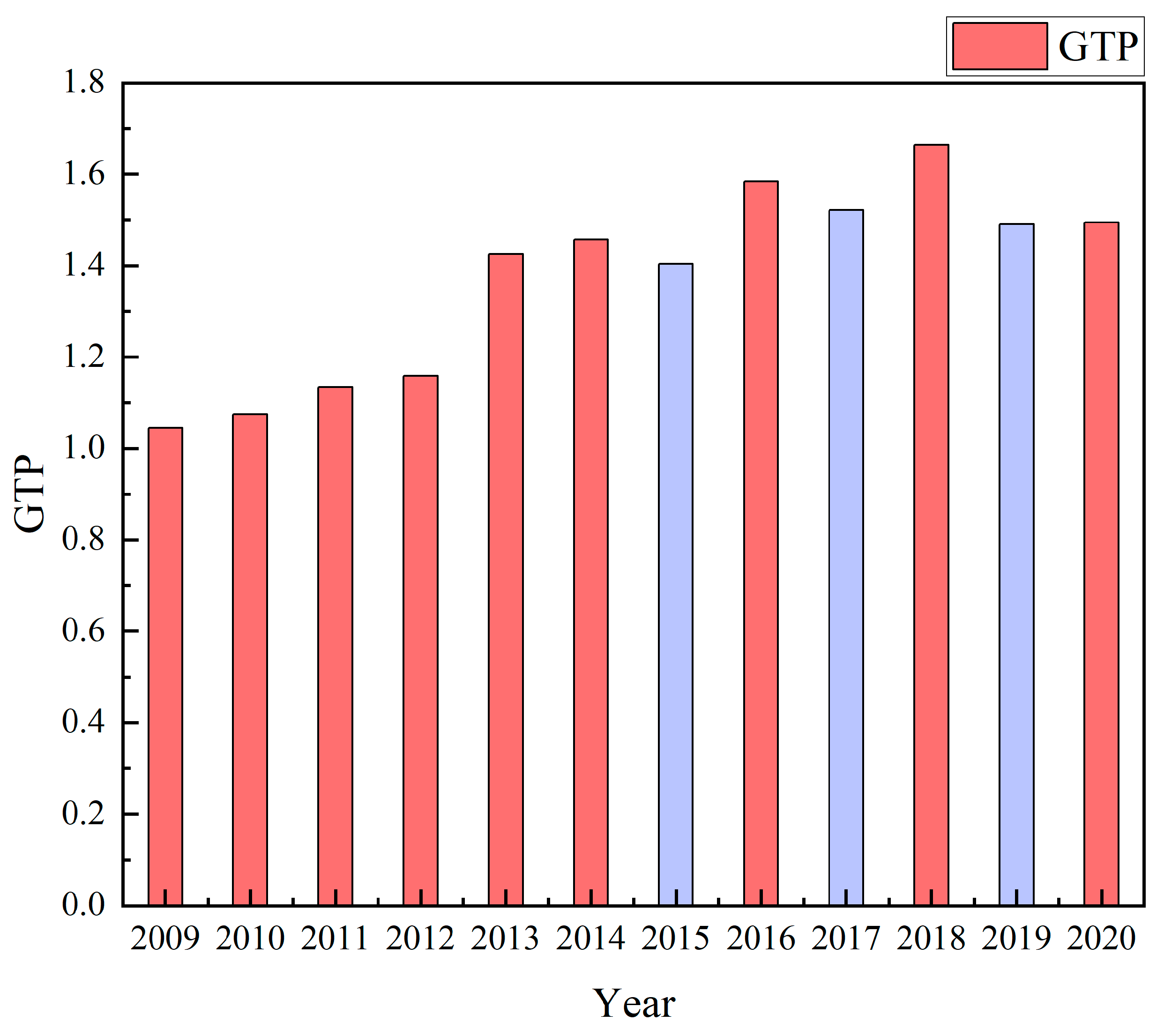
3.1. Temporal Variation of GTP in Mariculture

This study considers the undesirable output and uses MAXDEA8 software to calculate the GTP of China’s mariculture by using the EBM model. Furthermore, this study uses the GML index to decompose the GTFP for calculating the GTP index of mariculture. The GTP index of mariculture refers to the ratio of the change in GTP between two consecutive years in an area, and the result is a relative value. The analysis is as follows.

Table 1. The growth rate of green technology progress index in mariculture.

Provinces	2009	2010	2011	2012	2013	2014	2015	2016	2017	2018	2019	2020
Tianjin	1.003	0.999	1.059	1.019	1.133	1.007	1.048	1.023	0.913	1.020	0.967	0.930
Hebe	1.213	0.955	1.050	1.002	1.920	1.036	0.838	1.387	0.920	1.325	0.697	1.185
Liaoning	0.977	1.002	0.998	1.086	1.514	0.975	0.868	1.303	0.943	1.127	0.742	1.012
Jiangsu	0.918	1.031	1.064	1.035	1.338	0.916	0.867	1.310	0.970	1.023	0.914	0.900
Zhejiang	1.087	1.029	1.019	1.005	1.018	1.035	1.002	1.001	1.034	0.995	0.990	0.972
Fujian	1.048	1.110	1.071	1.075	1.117	1.107	1.021	1.050	0.897	1.089	0.996	0.989
Shandong	1.028	0.999	1.055	1.018	1.115	1.040	1.003	1.058	0.946	1.045	0.948	1.073
Guangdong	1.039	1.059	1.062	0.996	1.026	1.061	1.004	1.032	1.033	1.024	1.004	0.991
Guangxi	1.079	1.004	1.136	0.982	1.083	1.056	1.082	1.019	1.012	1.056	1.027	0.886
Hainan	1.048	1.120	1.031	1.010	1.050	0.992	1.013	1.005	1.009	1.008	0.987	0.974

shows the GTP index of mariculture in China’s ten coastal provinces from 2009 to 2020. A GTP index of less than 1 indicates that green technology progress has a downward trend, equal to 1 indicates that GTP has not changed, and greater than 1 indicates that GTP has improved. During the research period, the GTP index of China’s mariculture is generally maintained at more than 1, indicating that GTP in mariculture is at a high efficiency level and that the progress level is in a stage of development. The GTP index of China’s mariculture showed a significant fluctuation trend. For example, the GTP index of Tianjin, Hebei, Liaoning, and Jiangsu in 2010, 2014, 2015, and 2017 is generally less than 1, indicating that the GTP in these years is at a low efficiency level. Most provinces had a GTP index of less than 1 in 2019 and 2020, possibly due to the impact of COVID-19.

Table 2. Green technology progress in mariculture.

Provinces	2008	2009	2010	2011	2012	2013	2014	2015	2016	2017	2018	2019	2020
Tianjin	1.000	1.003	1.002	1.061	1.081	1.225	1.233	1.292	1.321	1.206	1.230	1.188	1.106
Hebei	1.000	1.213	1.158	1.216	1.218	2.340	2.424	2.032	2.818	2.593	3.435	2.396	2.840
Liaoning	1.000	0.977	0.980	0.978	1.061	1.607	1.567	1.360	1.772	1.671	1.883	1.397	1.413
Jiangsu	1.000	0.918	0.947	1.008	1.043	1.395	1.279	1.108	1.452	1.408	1.441	1.317	1.185
Zhejiang	1.000	1.087	1.118	1.139	1.145	1.165	1.206	1.208	1.209	1.251	1.244	1.231	1.197
Fujian	1.000	1.048	1.163	1.247	1.341	1.497	1.657	1.691	1.776	1.593	1.735	1.728	1.708
Shandong	1.000	1.028	1.027	1.084	1.103	1.230	1.280	1.284	1.358	1.285	1.343	1.273	1.366
Guangdong	1.000	1.039	1.101	1.168	1.164	1.195	1.267	1.273	1.314	1.356	1.389	1.395	1.383
Guangxi	1.000	1.079	1.083	1.230	1.208	1.308	1.381	1.495	1.524	1.542	1.628	1.671	1.480
Hainan	1.000	1.048	1.174	1.210	1.222	1.284	1.274	1.291	1.297	1.308	1.319	1.302	1.267

shows each province’s real GTP level in mariculture from 2008 to 2020. In terms of provinces, the growth trend of the GTP level in Hebei is larger than in other provinces. The GTP level in Hebei began to show a significant upward trend in 2013, widening the gap between it and other provinces. Its GTP reached the maximum value in 2018 at 3.435. In 2013, Hebei Province issued the Implementation Opinions of the People’s Government of Hebei Province on Promoting the Sustainable Development of Marine Fisheries [39], which proposed to change the development mode of fisheries and adhere to the policy of giving priority to ecology, which may be the main reason for the upward trend of its GTP level. The GTP levels of all other provinces were smaller at the beginning of the study period and showed a slow growth trend over time, fluctuating in the range of 0.918–1.883. Among them, the fluctuation trends of Liaoning, Fujian, and Guangxi are at a medium level, while Tianjin, Jiangsu, Zhejiang, Shandong, Guangdong, and Hainan have similar trends and are at the lowest fluctuation levels. In recent years, through measures such as increased financial investment in mariculture and the development of factory farming models, the level of green farming in all provinces has improved to varying degrees, and the GTP level has shown a fluctuating upward trend. Overall, the GTP level of all provinces showed a clear upward trend in 2013 and 2016, possibly because China began implementing the fisheries approach based on the principle of ecological priority and the marine economic powerful nation strategy in 2013 and implementing the 13th Five-Year Plan for National Fisheries Development in 2016 [40]. Under the influence of macro policies that focus on the ecological environment and the contribution of technology, the coastal provinces have made marine technology innovation and the transformation of marine science and technology achievements a vital part of their development, leading to an increased GTP level in mariculture. In order to understand the trend of GTP in China’s mariculture more intuitively, this study takes the average GTP in the coastal provinces from 2008 to 2020 as a measure of the total level of GTP in China’s mariculture, and its trend is shown in Figure 2.

In Figure 2, there is a fluctuating upward trend in the level of GTP in China’s mariculture from 2008 to 2018, with only a brief decline in 2015, 2017, and 2019. The COVID-19 epidemic negatively impacted environmentally sound invention efficiency [41]. So after the COVID-19 epidemic, the GTP of mariculture in China has been affected, but it also showed an evident recovery trend in 2020. Based on the growth in the later period of observation, it can be seen that GTP in China’s mariculture will reach a higher level of development in the future, further promoting a rapid increase in the TFP.

3.2. Spatial Variation of GTP in Mariculture

This section explores the spatial differences in mariculture GTP. This study uses MATLAB 2021 software to obtain the dynamic evolution of the Dagum Gini coefficient and its decomposition components.

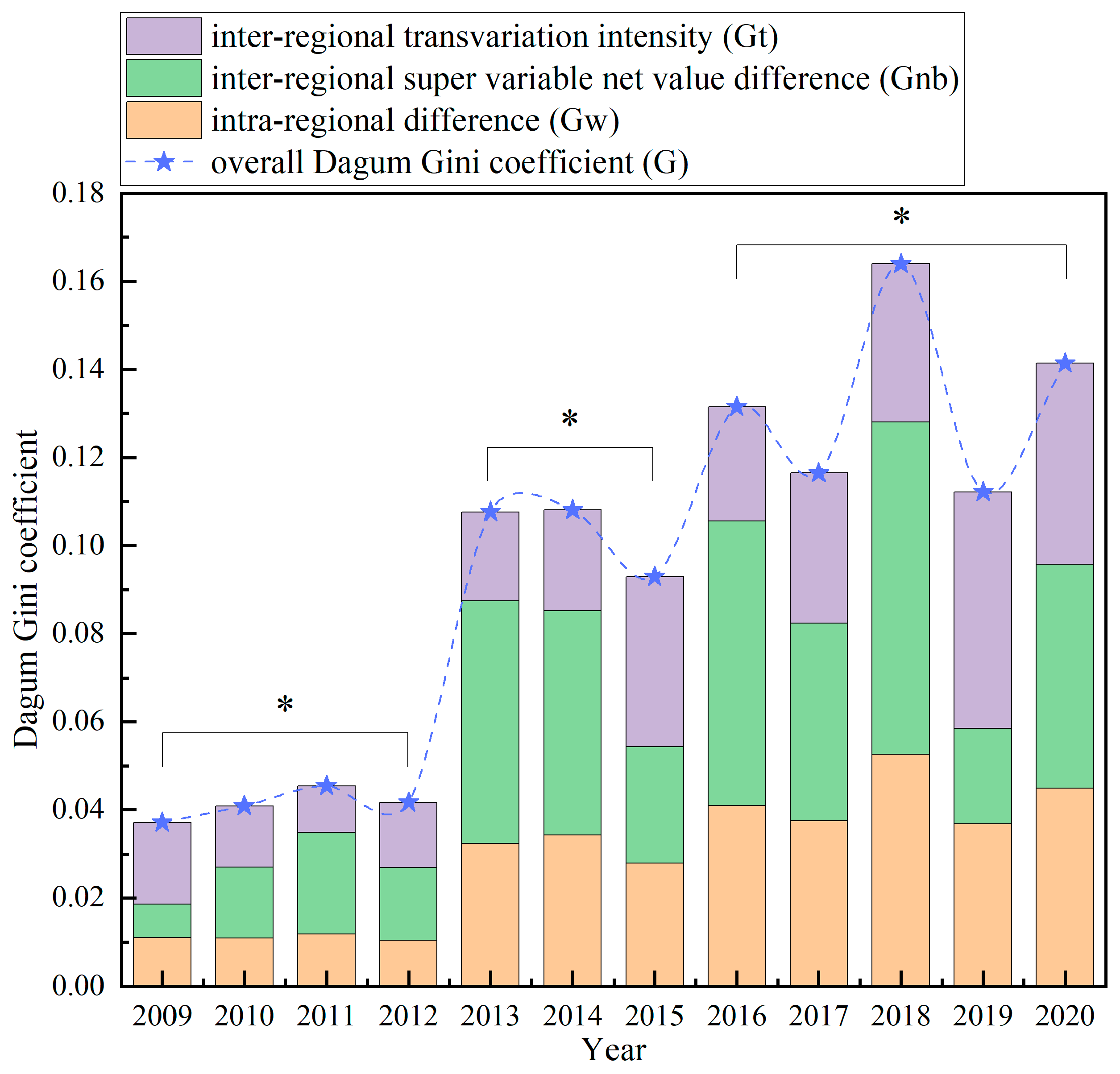
3.2.1. Overall Differences and Sources of GTP in Mariculture

The dashed line in Figure 3 reflects the G’s trend during the study period. It shows a fluctuating upward trend, with two relatively obvious turning points in 2013 and 2016. From 2009 to 2012, the G coefficient was stable at around 0.037–0.045, with slight regional differences. In 2013, the G coefficient jumped to 0.108 and fluctuated upward, reaching its maximum value (0.164) in 2018. The overall gap of mariculture GTP shows a clear dispersion trend over time.

The evolutionary trend of each source of GTP’s spatial variation is also reflected in Figure 3. During the study period, the annual average variance contributions of Gw, Gnb, and Gt of GTP spatial variation were 29.931%, 38.813%, and 31.256%, respectively. Thus, Gnb was the most significant source of GTP variation in coastal mariculture, accounting for about 40% of all sources of disparity. In addition, different sources of disparity showed different trends of change. Among them, Gw shows a steady and increasing trend. Its contribution rate rose from 29.711% in 2009 to 32.807% in 2019, with an average annual growth of 0.281% and a slight decline in 2020. Gnb and Gt’s contribution rates show significant fluctuations of 20–50%. Gnb’s contribution rate exceeds 35% in most years. In contrast, Gt’s contribution rate reached high values in 2009 and 2019 (49.871% and 47.893%, respectively), while there has been a significant decreasing trend in recent years.

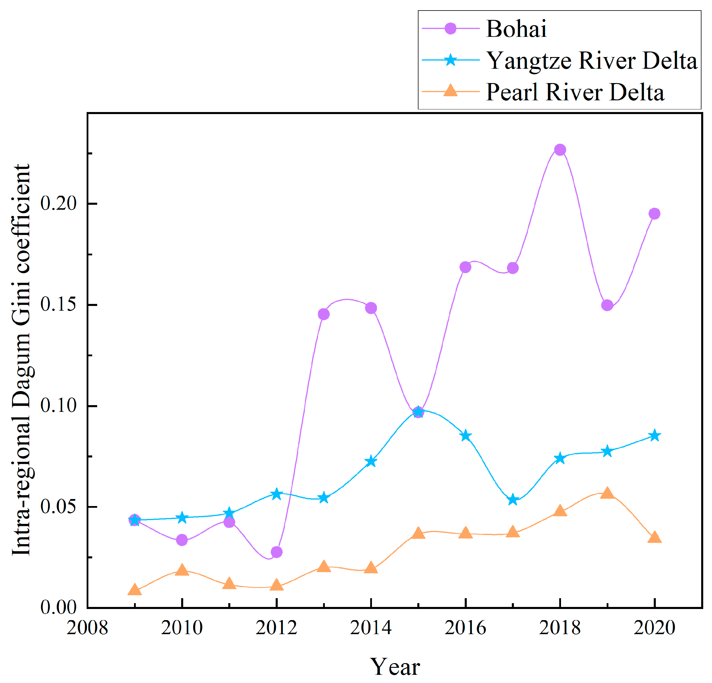
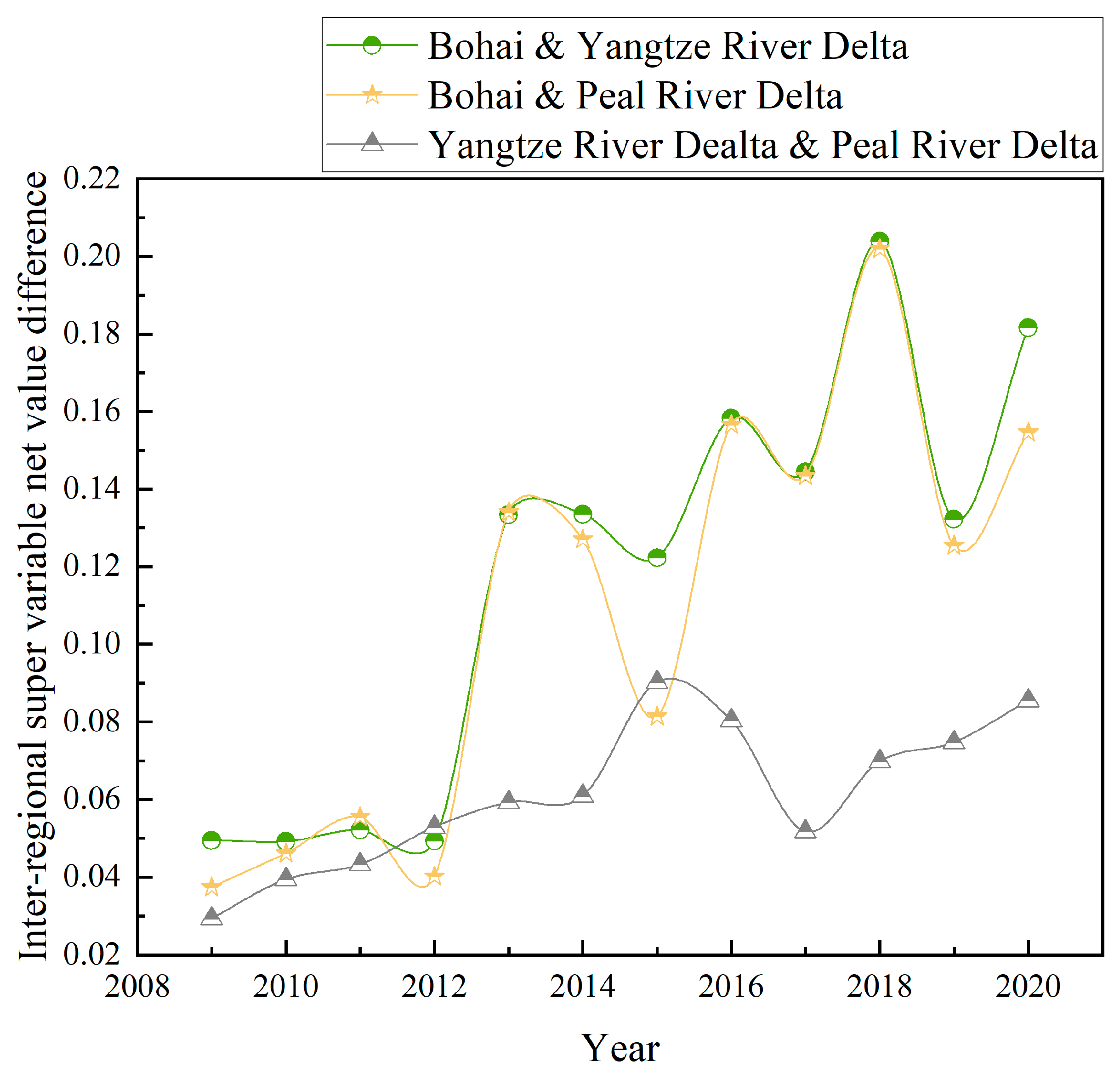
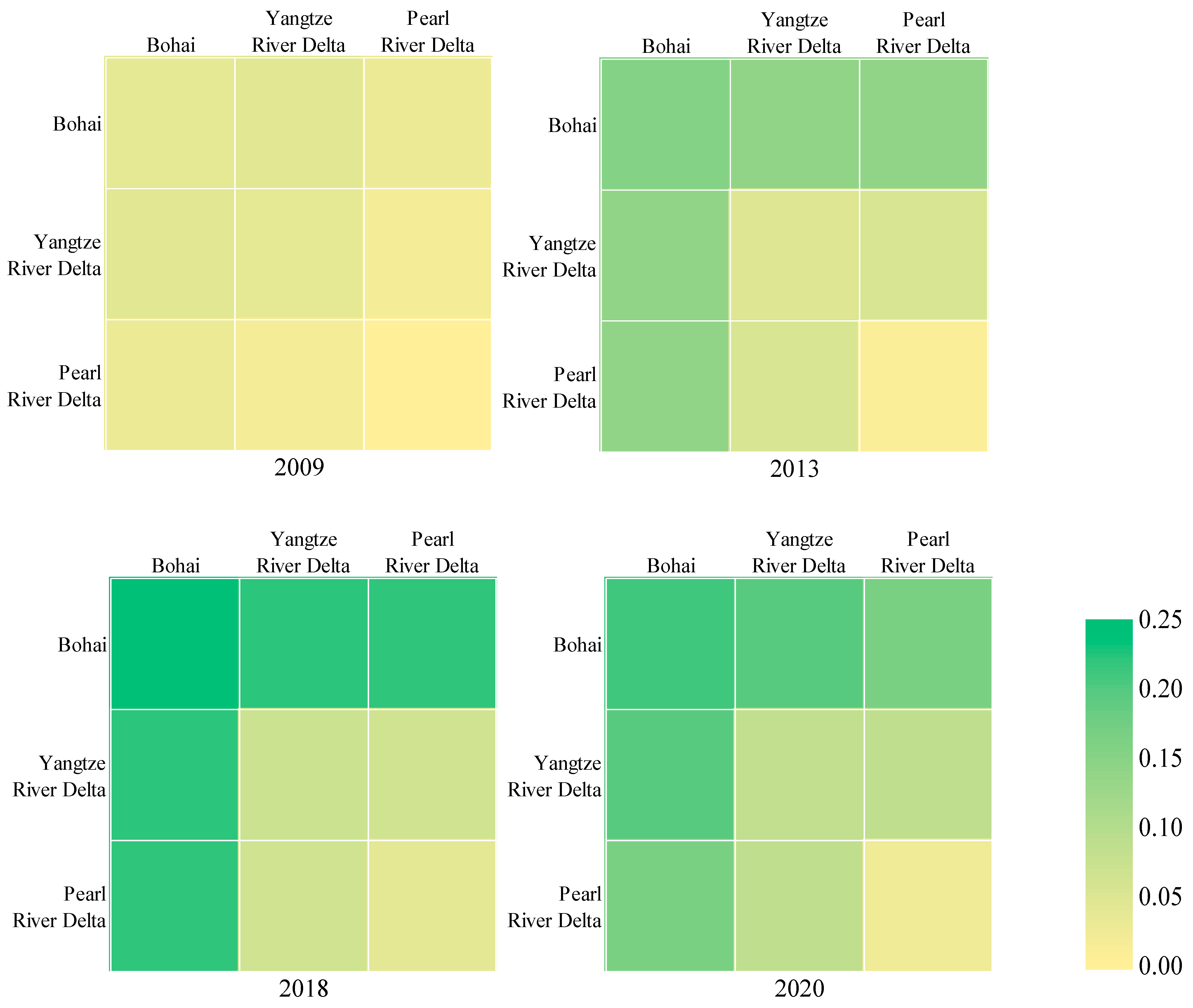
3.2.2. Intra-Regional and Inter-Regional Variation in Mariculture GTP

Figure 4 and Figure 5 depict the trends of Gw and Gnb’s variation in mariculture GTP in more detail. The Gw in GTP is ranked in descending order: Bohai region, Yangtze River Delta, and Pearl River Delta. Gw in the Pearl River Delta is smaller than the other two regions in the same period and changes smoothest. Gw in the Bohai region has the most significant changes and is significantly higher than in other regions after 2012. Gw in the Yangtze River Delta area has fluctuated and increased recently. Overall, the Bohai region is the primary source of the rising Gw during the study period.

From the evolutionary trend of Gnb of mariculture GTP, the ranking of Gnb values in descending order is as follows: Bohai region–Yangtze River Delta, Bohai region–Pearl River Delta, and Yangtze River Delta–Pearl River Delta. Each group shows a fluctuating upward trend. The first two groups have similar change trends and are the primary source of Gnb. Both groups show a significant gap after 2012. The changing trend of Gnb in the Yangtze River Delta–Pearl River Delta area is relatively flat.

According to Figure 4 and Figure 5, 2013 and 2018 are the years in which Gw and Gnb show a jump and the highest values, respectively. To reflect the overall changes during the study period and to represent the spatial differences of GTP more visually, we chose 2009, 2013, 2018, and 2020 as representative years to plot the heat map of Gw and Gnb (Figure 6). Through the shades of color, the heat map visually reflects the differences within regions (diagonal color changes, i.e., Gw) and between regions (upper and lower triangles symmetrically reflect the differences between each pair of regions, i.e., Gnb). Figure 6 is presented in a symmetrical form for aesthetic purposes. It is clear that the GTP difference both within the Bohai region and between it and other regions widened significantly in 2013 and reached its maximum in 2018. Mariculture GTP still shows significant spatial differences in recent years.

3.3. Convergence Results

Section 3.2 shows that there is a significant spatial difference in mariculture GTP. Next, the convergence characteristics of the spatial differences are further examined through $\mathsf{\sigma }$ and β convergence.

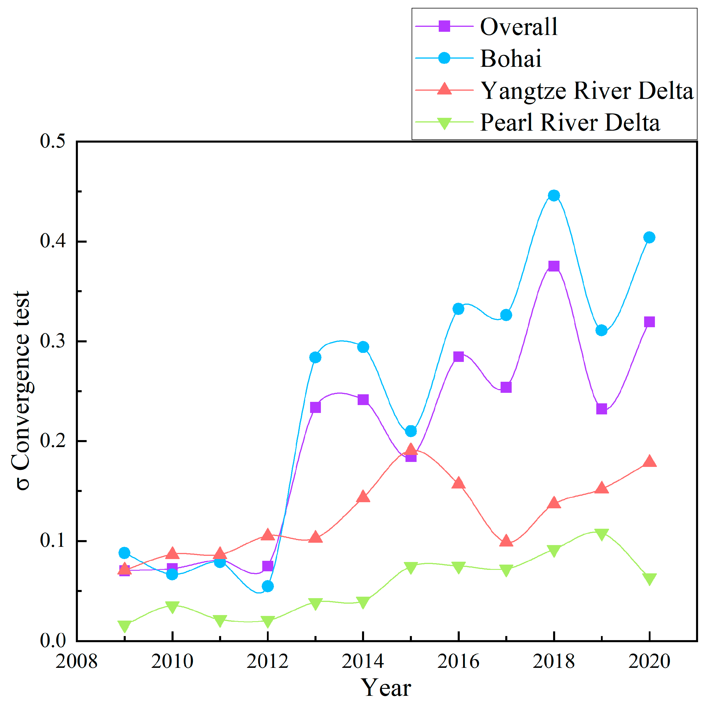
3.3.1. σ Convergence Results

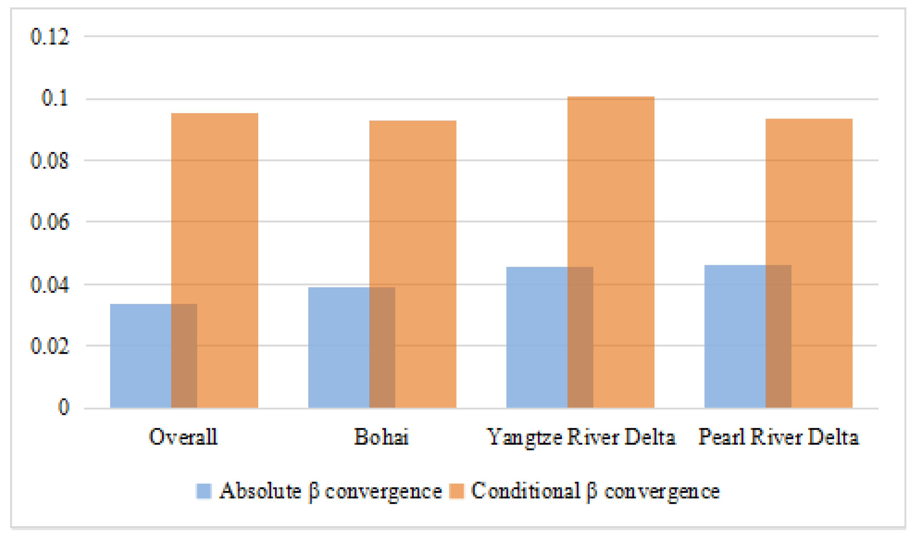
According to Formula (18), this study calculates the $\mathsf{\sigma }$ value of the mariculture sector’s GTP for the Bohai region, Yangtze River Delta, and Pearl River Delta to investigate whether the degree of dispersion of GTP in different regions will continue to shrink over time.

Figure 7 shows the $\mathsf{\sigma }$ convergence test results of GTP in mariculture. Overall, the value from 2009 to 2020 increased from 0.0702 to 0.3194. The entire observation range showed a fluctuating but rising trend without significant σ convergence. It shows that a nationwide convergence trend is not apparent, and the differences in GTP in mariculture have not decreased over time. Regarding the three regions, although the fluctuation of values in the observation period is inconsistent, the overall trend for 2009–2020 shows an increase, indicating that the dispersion of GTP in mariculture among the three regions is increasing over time. Among them, both the Yangtze River Delta and Pearl River Delta regions presented a low σ convergence in the starting year 2009 (0.0708 and 0.0162, respectively), while Bohai presented the lowest σ convergence in 2012 (0.0546). Bohai and Pearl River Delta reached the highest σ convergence in 2018 and 2019 (0.4459 and 0.1078, respectively), while the Yangtze River Delta reached the highest level of σ convergence in 2015 (0.1905). The trend of σ convergence is closest between the Bohai Sea and the overall coastal area.

3.3.2. Absolute $\mathsf{\beta }$ Convergence Results

Based on the OLS regression model, this study analyzes the spatial convergence of GTP in mariculture overall and the three regions. The absolute $\mathsf{\beta }$ convergence results are shown in

Table 3. Absolute β convergence test of green technology progress in mariculture.

Regional	Coefficient	t-Statistic	p-Value	Convergence Rate	Convergence or Divergence
Overall	−0.3304	−4.44	0.000	0.0334	convergence
Bohai	−0.3750	−3.02	0.003	0.0392	convergence
Yangtze River Delta	−0.4221	−3.03	0.002	0.0457	convergence
Pearl River Delta	−0.4254	−2.39	0.017	0.0462	convergence

.

Table 3 shows GTP’s absolute $\mathsf{\beta }$ convergence results in China’s mariculture. The absolute $\mathsf{\beta }$ convergence coefficient of the overall GTP and that of the three regions have significant convergence at the 5% level without considering their economic development levels and characteristics. It indicates that the growth rates of differences in mariculture GTP among regions are decreasing, suggesting a catch-up phenomenon from low to high levels. That is, the growth rate of GTP in low-level mariculture regions is higher than in high-level regions.

3.3.3. Conditional $\mathsf{\beta }$ Convergence Results

Based on the absolute $\mathsf{\beta }$ convergence, the individual fixed effect is added to analyze the convergence of GTP, which is more relevant to the actual situation.

Table 4. Conditional $\mathsf{\beta }$ convergence test for green technology progress in mariculture.

Regional	Coefficient	t-Statistic	p-Value	Convergence Rate	Convergence or Divergence
Overall	−0.6805	−10.22	0.000	0.0951	convergence
Bohai	−0.6721	−6.28	0.008	0.0929	convergence
Yangtze River Delta	−0.7003	−12.70	0.006	0.1004	convergence
Pearl River Delta	−0.6742	−14.05	0.005	0.0935	convergence

shows GTP’s conditional $\mathsf{\beta }$ convergence results in China’s mariculture. The conditional $\mathsf{\beta }$ convergence coefficient of the overall GTP and that of the three regions have significant convergence at the 1% level. It suggests that, due to the different levels and characteristics of economic development, each province’s GTP growth rate converges to its respective steady-state equilibrium level over time.

Further comparing the convergence rates of absolute $\mathsf{\beta }$ convergence and conditional $\mathsf{\beta }$ convergence among different coastal regions (Figure 8), the absolute value of the convergence rate of conditional $\mathsf{\beta }$ convergence exceeds that of absolute $\mathsf{\beta }$ convergence. It means that the growth rate of mariculture GTP will first reach their respective steady-state levels under their resources and environmental constraints and then approach a unified steady-state equilibrium level. Comparing the three regions, the Pearl River Delta has the highest absolute $\mathsf{\beta }$ convergence rate, followed by the Yangtze River Delta and the Bohai region. The Yangtze River Delta has the highest conditional $\mathsf{\beta }$ convergence rate, followed by the Pearl River Delta and the Bohai region. These differences in convergence rates may be due to differences in the economic development level and characteristics of mariculture among different regions. Therefore, these provinces should formulate mariculture development policies according to their development conditions.

4. Conclusions

In this study, the EBM-Malmquist model was used to calculate the GTP in mariculture of China’s ten provinces from 2008 to 2020, and the GTP’s spatial differences were analyzed with the help of Dagum Gini coefficient, as well as different convergence models were used to explore the convergence of spatial differences of GTP among coastal areas. The following conclusions can be drawn. Regarding the temporal and spatial trends of China’s mariculture GTP, GTP showed a fluctuating upward trend during the study period, with an average annual growth rate of 4.12%. GTP in mariculture has great growth potential and good development prospects. In addition, there was a significant spatial variation in GTP. The overall differences show a clear trend of dispersion over time. The sources of variation are Gnb, Gt, and Gw from largest to smallest. Among them, the Bohai region is the primary source of intra-regional variation, while the Bohai–Yangtze Delta and the Bohai–Pearl River Delta areas are the primary sources of inter-regional variation. In terms of the convergence characteristics of the spatial differences of GTP, the degree of dispersion of GTP in mariculture between regions has not decreased with time; in other words, there is no apparent σ convergence. Additionally, there is an absolute $\mathsf{\beta }$ convergence and a conditional $\mathsf{\beta }$ convergence of GTP in mariculture between regions, and the absolute value of the convergence rate of conditional $\mathsf{\beta }$ convergence exceeds that of absolute $\mathsf{\beta }$ convergence. Therefore, the growth rate of regional differences will first converge to each region’s steady-state level and converge to a steady-state equilibrium level in the long run.

The above results provide important implications for China’s mariculture’s sustainable and healthy development. Firstly, to strengthen regional cooperation and exchange, the analysis of the convergence of GTP in mariculture indicates the existence of a catch-up phenomenon from low-level areas to high-level areas. Therefore, we should pay great attention to the technology spillover effect from high-level areas and speed up the development of GTP in low-level areas by strengthening regional exchanges and cooperation, accelerating the transformation and upgrading of mariculture, improving the GTFP of the mariculture industry, and promoting the efficient development of mariculture. Secondly, interregional development of mariculture must not be pursued with absolute unity of development goals and speed; instead, developmental plans should pay attention to local conditions and consider the differences in economic development levels among regions.

References

1. Mc Carthy, U.; Uysal, I.; Badia-Melis, R.; Mercier, S.; O’Donnell, C.; Ktenioudaki, A. Global food security—Issues, challenges and technological solutions. Trends Food Sci. Technol. 2018, 77, 11–20. [Google Scholar] [CrossRef]
2. Liang, X.; Jin, X.; Han, B.; Sun, R.; Xu, W.; Li, H.; He, J.; Li, J. China’s food security situation and key questions in the new era: A perspective of farmland protection. J. Geogr. Sci. 2022, 32, 1001–1019. [Google Scholar] [CrossRef]
3. Yu, J.; Han, Q. Food security of mariculture in China: Evolution, future potential and policy. Mar. Policy 2020, 115, 103892. [Google Scholar] [CrossRef]
4. Meng, W.; Feagin, R.A. Mariculture is a double-edged sword in China. Estuar. Coast. Shelf Sci. 2019, 222, 147–150. [Google Scholar] [CrossRef]
5. Yuan, B.; Yue, F.; Wang, X.; Xu, H. The Impact of Pollution on China Marine Fishery Culture: An Econometric Analysis of Heterogeneous Growth. Front. Mar. Sci. 2021, 8, 760539. [Google Scholar] [CrossRef]
6. Edwards, P. Aquaculture environment interactions: Past, present and likely future trends. Aquaculture 2015, 447, 2–14. [Google Scholar] [CrossRef]
7. Yu, L.; Liu, D.; Xu, N. Special aquatic products supply chain coordination considering bilateral green input in the context of high-quality development. Int. J. Found. Comput. Sci. 2022, 33, 819–844. [Google Scholar] [CrossRef]
8. Xu, J.; Qin, T. Research on the efficiency of marine aquaculture production in Guangdong province based on the Malmquist index. Ocean. Dev. Manag. 2018, 35, 98–103. [Google Scholar]
9. Guo, W.; Dong, S.; Qian, J.; Lyu, K. Measuring the Green Total Factor Productivity in Chinese Aquaculture: A Zofio Index Decomposition. Fishes 2022, 7, 269. [Google Scholar] [CrossRef]
10. Ji, J.; Zeng, Q. A study on the total factor productivity of China’s Mariculture—Considered undesirable outputs based on global Malmquist-Luenberger index. J. Ocean. Univ. China (Soc. Sci.) 2017, 1, 43–48. [Google Scholar]
11. Sun, Y.; Ji, J. Measurement and analysis of technological progress bias in China’s mariculture industry. J. World Aquacult. Soc. 2022, 53, 60–76. [Google Scholar] [CrossRef]
12. Ji, J.; Sun, Y.; Yin, X. Study on green output bias of China’s mariculture technological progress. Environ. Sci. Pollut. Res. 2022, 29, 60558–60571. [Google Scholar] [CrossRef]
13. Bouwman, L.; Beusen, A.; Glibert, P.M.; Overbeek, C.; Pawlowski, M.; Herrera, J.; Mulsow, S.; Yu, R.; Zhou, M. Mariculture: Significant and expanding cause of coastal nutrient enrichment. Environ. Res. Lett. 2013, 8, 044026. [Google Scholar] [CrossRef]
14. Xu, J.; Han, L.; Yin, W. Research on the ecologicalization efficiency of mariculture industry in China and its influencing factors. Mar. Policy 2022, 137, 104935. [Google Scholar] [CrossRef]
15. Liang, Y.; Cheng, X.; Zhu, H.; Shutes, B.; Yan, B.; Zhou, Q.; Yu, X. Historical evolution of mariculture in China during past 40 years and its impacts on eco-environment. Chin. Geogr. Sci. 2018, 28, 363–373. [Google Scholar] [CrossRef] [Green Version]
16. Zhang, J.; Wu, W.; Li, Y.; Liu, Y.; Wang, X. Environmental effects of mariculture in China: An overall study of nitrogen and phosphorus loads. Acta Oceanol. Sin. 2022, 41, 4–11. [Google Scholar] [CrossRef]
17. Wang, P.; Ji, J. Research on China’s mariculture efficiency evaluation and influencing factors with undesirable outputs—An empirical analysis of China’s ten coastal regions. Aquacult. Int. 2017, 25, 1521–1530. [Google Scholar] [CrossRef]
18. Liu, Y.; Wang, X.; Wu, W.; Yang, J.; Wu, N.; Zhang, J. Experimental Study of the Environmental Effects of Summertime Cocultures of Seaweed Gracilaria lemaneiformis (Rhodophyta) and Japanese Scallop Patinopecten yessoensis in Sanggou Bay, China. Fishes 2022, 6, 53. [Google Scholar] [CrossRef]
19. Ji, J.; Li, Y. Research on green technology progress measurement and influencing factors in marine aquaculture industry in China. J. Ocean. Univ. China (Soc. Sci.) 2019, 2, 45–50. [Google Scholar]
20. Ren, W.; Zeng, Q. Is the green technological progress bias of mariculture suitable for its factor endowment?—Empirical results from 10 coastal provinces and cities in China. Mar. Policy 2021, 124, 104338. [Google Scholar] [CrossRef]
21. Tone, K.; Tsutsui, M. An epsilon-based measure of efficiency in DEA—A third pole of technical efficiency. Eur. J. Oper. Res. 2010, 207, 1554–1563. [Google Scholar] [CrossRef]
22. He, Q.; Du, J. The impact of urban land misallocation on inclusive green growth efficiency: Evidence from China. Environ. Sci. Pollut. Res. 2021, 29, 3575–3586. [Google Scholar] [CrossRef] [PubMed]
23. Oh, D.H. A global Malmquist-Luenberger productivity index. J. Prod. Anal. 2010, 34, 183–197. [Google Scholar] [CrossRef]
24. Vassdal, T.; Sørensen Holst, H.M. Technical progress and regress in Norwegian salmon farming: A Malmquist index approach. Mar. Resour. Econ. 2011, 26, 329–341. [Google Scholar] [CrossRef]
25. Ji, J.; Liu, L.; Xu, Y.; Zhang, N. Spatio-Temporal disparities of mariculture area production efficiency considering undesirable output: A case study of China’s east coast. Water 2022, 14, 324. [Google Scholar] [CrossRef]
26. Chen, Y.; Song, G.; Zhao, W.; Chen, J. Estimating pollutant loadings from mariculture in China. Mar. Environ. Sci. 2016, 35, 1–6. [Google Scholar] [CrossRef]
27. Fan, S.; Zhang, X.; Robinson, S. Structural change and economic growth in China. Rev. Dev. Econ. 2003, 7, 360–377. [Google Scholar] [CrossRef]
28. Dagum, C. A new approach to the decomposition of the Gini income inequality ratio. Empir. Econ. 1997, 22, 515–531. [Google Scholar] [CrossRef]
29. Ji, J.; Wang, D. Regional differences, dynamic evolution, and driving factors of tourism development in Chinese coastal cities. Ocean Coast. Manag. 2022, 226, 106262. [Google Scholar] [CrossRef]
30. Lerman, R.I.; Yitzhaki, S. Improving the accuracy of estimates of Gini Coefficients. J. Econ. 1989, 42, 43–47. [Google Scholar] [CrossRef]
31. Yu, C.; Wenxin, L.; Khan, S.U.; Yu, C.; Jun, Z.; Yue, D.; Zhao, M. Regional Differential Decomposition and Convergence of Rural Green Development Efficiency: Evidence from China. Environ. Sci. Pollut. Res. 2020, 27, 22364–22379. [Google Scholar] [CrossRef]
32. Mohammadi, H.; Ram, R. Cross-country convergence in energy and electricity consumption, 1971–2007. Energy Econ. 2012, 34, 1882–1887. [Google Scholar] [CrossRef]
33. Zhuang, W.; Wang, Y.; Lu, C.C.; Chen, X. The green total factor productivity and convergence in China. Energy Sci. Eng. 2022, 10, 2794–2807. [Google Scholar] [CrossRef]
34. Zhu, L.; Shi, R.; Mi, L.; Liu, P.; Wang, G. Spatial Distribution and Convergence of Agricultural Green Total Factor Productivity in China. Int. J. Environ. Res. Public Health 2022, 19, 8786. [Google Scholar] [CrossRef]
35. Barro, R.J.; Sala-i-Martin, X. Convergence. J. Political Econ. 1992, 100, 223–251. [Google Scholar] [CrossRef]
36. Hu, J. Green productivity growth and convergence in Chinese agriculture. J. Environ. Plann. Manag. 2023, 2, 1–30. [Google Scholar] [CrossRef]
37. Cheng, Z.; Liu, J.; Li, L.; Gu, X. Research on meta-frontier total-factor energy efficiency and its spatial convergence in Chinese provinces. Energy Econ. 2020, 86, 104702. [Google Scholar] [CrossRef]
38. Jiang, L.; Folmer, H.; Ji, M.; Zhou, P. Revisiting cross-province energy intensity convergence in China: A spatial panel analysis. Energy Policy 2018, 121, 252–263. [Google Scholar] [CrossRef]
39. Lin, X.; Zheng, L.; Li, W. Measurement of the contributions of science and technology to the marine fisheries industry in the coastal regions of China. Mar. Policy 2019, 108, 103647. [Google Scholar] [CrossRef]
40. Cao, L.; Chen, Y.; Dong, S.; Hanson, A.; Huang, B.; Leadbitter, D.; Little, D.C.; Pikitch, E.K.; Qiu, Y.S.; de Mitcheson, Y.S.; et al. Opportunity for marine fisheries reform in China. Proc. Natl. Acad. Sci. USA 2017, 114, 435–442. [Google Scholar] [CrossRef] [Green Version]
41. Wei, X.; Liu, R.; Lin, Z. “Crisis” or “opportunity”? COVID-19 pandemic’s impact on environmentally sound invention efficiency in China. Front. Public Health 2022, 10, 1102680. [Google Scholar] [CrossRef] [PubMed]
Figure 1. Graphical representation of the Global Malmquist-Luenberger index.
Fishes 08 00338 g001
Figure 2. The trend of green technology progress in China’s mariculture.
Fishes 08 00338 g002
Figure 3. Overall differences and sources of Dagum Gini coefficient (“*” denotes three different periods divided by the trend of the Dagum Gini coefficient).
Fishes 08 00338 g003
Figure 4. The trend of intra-regional difference changes.
Fishes 08 00338 g004
Figure 5. The trend of inter-regional super variable net value difference changes.
Fishes 08 00338 g005
Figure 6. Heat map of regional differences in green technology progress.
Fishes 08 00338 g006
Figure 7. The σ convergence test results of green technology progress in mariculture.
Fishes 08 00338 g007
Figure 8. Comparison of the convergence rates between absolute β convergence and conditional β convergence.
Fishes 08 00338 g008