Environmental Factors Determine Tuna Fishing Vessels’ Behavior in Tonga

Abstract

Comprehending the spatial distribution of human fishing endeavors holds significant importance in the context of monitoring fishery resources and implementing spatial management measures. To gain insights into the spatial arrangement of tuna longline activities within the exclusive economic zones of Tonga and their correlation with the marine environment, this study utilizes data from the Tonga Tuna Longline Fisheries spanning from 2002 to 2018. The data are employed to extract information about the spatial distribution of fishing efforts and coupled with 15 marine environmental variables covering both sea surface and subsurface conditions. This study employs boosted regression trees (BRT) and general additive models (GAM) to establish the non-linear relationships between the distribution of fishing effort and marine environmental factors. Furthermore, it examines and analyzes the ecological niche occupied by tuna longline vessels in high-sea environments. The outcomes of the factor analysis indicate that the most important factors influencing the fishing efforts of tuna longliners are the dissolved oxygen content at the sea surface and latitude. These two factors contribute significantly, accounting for 19.06% and 18.62% of the fishing efforts of vessels, respectively, followed by distance to ports, longitude, and dissolved oxygen at 100 m depth, contributing 10.77%, 7.07%, and 6.30%, respectively. The sea surface chlorophyll, ocean current at 100 m depth, and mixed layer depth contributed the least, 3.63%, 2.13%, and 1.72, respectively. In terms of space and time, tuna longliners are more likely to operate in the 18–22° S latitudinal and 172–178° W longitudinal region, and fishing efforts increased in the months from March to August. The spatial distribution of the fishing efforts modeled for fishing vessels in 2018 is predicted to have good spatial distribution with the actual fishing efforts of these vessels. This research aids in comprehending the environmental impacts resulting from shifts in the spatial distribution of tuna longline vessels, offering valuable insights for the effective management of tuna longline fisheries in Tonga.

1. Introduction

Being a crucial economic asset among marine fishery resources, tuna (Thunnini) stands out as the most prized and commercially valuable fish globally [1,2,3]. Likewise, the Western and Central Pacific Ocean (WCPO) boasts the world’s largest tuna industry, with yearly catches surpassing 2 million metric tons (mt), constituting roughly half of the global tuna harvest [4]. Furthermore, at a worldwide level, the exclusive economic zones (EEZs) of the Pacific Island countries (PICs) contain the most significant tuna reserves, contributing approximately 65% to 75% of the total tuna catches in the WCPO [5,6]. Tonga’s primary commercial fishery revolves around tuna production, amounting to an estimated 2000 mt annually [7,8]. However, tuna populations have seen an average decrease of 60% over the past five decades [9,10]. In this setting, the sustainable management of tuna resources has emerged as a top priority on national, regional, and global scales [11,12,13].

Using satellite-based oceanographic data has been recognized as a potential tool that could enhance both tuna production and management results [14,15,16]. In terms of management results, the utilization of satellite-based oceanographic data can contribute to more effective fisheries management by providing real-time information on relevant environmental variables. Such information aids in the identification of optimal fishing grounds, helping fisheries managers implement sustainable practices [15,16]. Research indicates that the surface and subsurface layers of oceanic environments significantly affect the distribution and presence of tuna in the water column [17,18]. The physiological functions of tuna are directly impacted by the temperature of the sea surface [15,19]. The concentration of Chl-a has been identified as a factor influencing the spatial and temporal distribution of tuna in the WCPO and the East Pacific Ocean [19,20,21]. The catch rate of yellow and bigeye tuna in the Indian Ocean has been found to be influenced by bathymetry, typically resulting in higher catch per unit effort (CPUE) as the size of steep bathymetric zones increases [22]. Ocean near-surface advection and converging and diverging flows are connected to variations in sea surface height, where tuna use these variations as cues to locate regions where food is abundant [23]. Ocean currents impact the movement of phytoplankton and small pelagic fish, thereby influencing the distribution of higher trophic-level marine animals [24]. The distribution and presence of tuna in the ocean environment are also influenced by dissolved oxygen levels [25] and salinity [26,27].

Fishermen rely on their knowledge and the prevailing marine conditions to locate and catch fish. Fishing vessels adapt their position and fishing techniques in response to the changing spatial distribution of tuna resources [28,29]. It is crucial for ecosystem-based tuna fisheries management to encompass the monitoring of fishing activities of tuna vessels [30,31]. Therefore, in order to effectively and sustainably manage marine resources like tuna, ecosystem-based management must include an awareness of fishing activities, such as time at sea and fishing methods [32,33,34]. An understanding of the connection between the operations of tuna fishing vessels and the environment can yield more accurate fishery data for effective management of fishing intensity and fishery resources.

Research indicates that data gathered from fishing vessels, such as distance to ports, fishing locations, fishing gears and methods, CPUE, fishing duration, and time, to some extent, reflect the direct interplay between vessel fishing practices and socio-economic implications [35,36] and various environmental factors [37,38,39,40]. The studies mentioned above suggest that the allocation of fishing effort is shaped by the environment and can be elucidated and forecasted by utilizing species distribution models in conjunction with data pertaining to environmental conditions and fishing observations. Studies have indicated that various environmental factors, including temperature, sea surface height, salinity, chlorophyll levels, dissolved oxygen, mixed layer depth, and sea surface currents, impact the habitat of tuna in the Western–Central Pacific Ocean (WCPOC) and other places [41,42,43]. Water depths also play an important role in influencing the spatial and temporal distributions of tuna [44,45,46].

Nicolas et al. (2011) [47] utilized vessel monitoring system (VMS) data for a study aimed at quantifying the spatial patterns of Seschel tuna fishing in the Indian Ocean. They employed a Bayesian state-space model to categorize the movement and activities of vessels at sea into three distinct phases: sailing, tracking, and fishing. The study delved into a statistical analysis of the spatial trajectory distribution by examining the vessel’s duration at sea in each location. Zhang et al. [48] conducted a spatial examination of tuna vessels’ fishing activities in the Western and Central Pacific. They employed vessel trajectory data obtained from the automatic identification system (AIS) and utilized the duration of time vessels spent at sea as a measure of fishing effort, establishing correlations with data related to tuna production and time at sea in the Western and Central Pacific Ocean (WCPO). The results indicate a strong positive correlation (r > 0.8). Consequently, it is justifiable to characterize the duration vessels spend at sea for tuna fishing as a measure of fishing effort. Fishing effort, here, is defined as the measure of how much tuna is caught and changes in the spatial behavior of fishing vessels over a defined period of time. Hsu et al. (2021) [41] utilized longline vessel fishing effort data to construct a habitat index model, leading to a highly accurate prediction of the spatial and temporal distribution of skipjack fisheries in the WCPO, and the results demonstrated that fishing effort data are better than catch data in this context. This suggests that the model response to environmental factors, built using vessel fishing effort data, can effectively aid in comprehending the spatial dispersion of fishery resources and environmental influences.

Generalized additive models (GAMs) have been successfully used to describe the habitat preferences of target and non-target species and have often been used to predict species distributions [14,49,50,51]. GAMs enable the exploration of non-linear connections between response variables, such as the CPUE of tuna species, and various sets of predictors. This approach does not necessitate an explicit definition of the relationship form, thereby enriching our understanding of how environmental variables impact the distribution and abundance of populations [50,51,52]. These models are semi-parametric expansions of generalized linear models, assuming that the functions are additive and the components exhibit smoothness [53]. GAMs possess the capability to manage extremely non-linear and non-monotonic connections between response variables and explanatory factors, rendering them well-suited for representing the inherent relationships within ecological systems [54].

In Tonga (Figure 1), the primary fishing techniques used for tuna are predominantly longlining and pole fishing, with longlining being the dominant method [8]. Currently, when examining global tuna longline fishing, there is a scarcity of research on how human fishing activities make use of resources on the high seas, particularly in regional and national reports. The Western and Central Pacific regions are the primary source of tuna, yet the relationship between the distribution of tuna longline fishing and environmental factors has rarely been studied. In this study, we investigate the fishing effort data on tuna longline fishing in Tonga. Using GAMs, we build environmental impact models for vessel operation distribution and compare their accuracy. These models are then used to extract fishery-related information and make predictive fishing effort maps. Analyzing the environmental factors that influence the spatial arrangement of tuna longline fleets offers valuable support toward the aims of tuna fishery management in Tonga. These aims include the promotion, sustainability, ecosystem protection, and economic viability of the nation’s tuna resources [8].

2. Materials and Methods

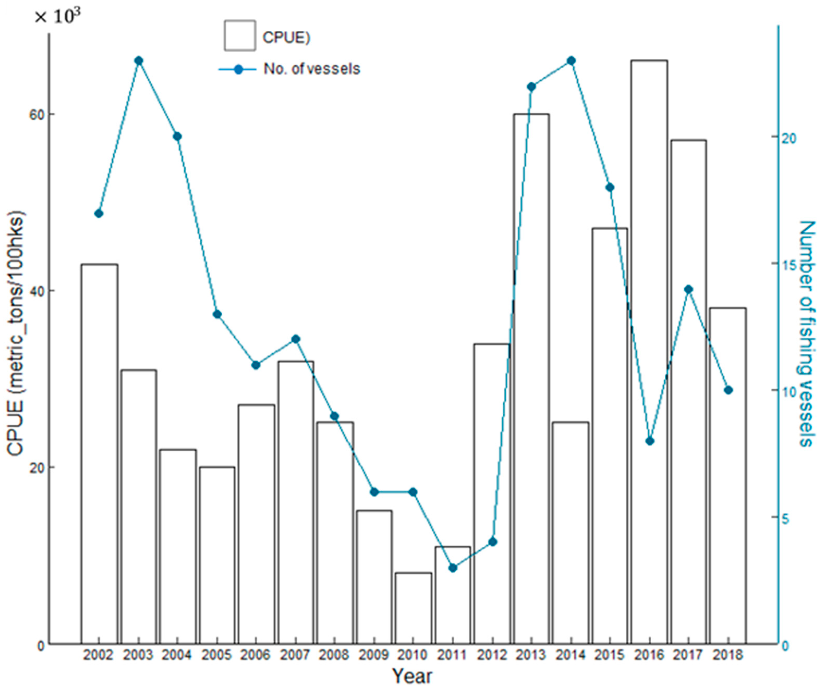
2.1. Catch per Unit Effort Data

The fishing effort information in this paper uses the daily operating time data compiled by the Tonga tuna longline fishery and provided by the Tonga Ministry of Fisheries and the South Pacific Community Office in New Caledonia with a spatial grid accuracy of 1° from 2002 to 2018. The Tonga longline vessels mainly catch albacore (Thunnus alalunga), bigeye (Thunnus obesus), skipjack (Katsuwonus pelamis), and yellowfin (Thunnus albacares) [8]. The data include daily fishing positions (latitude and longitude), fishing effort (in number of hooks), fishing date (in days, months, and years), catch (in numbers and kilograms), and number of vessels per fishing day. In order to simplify calculations involving large numbers, the effort rate was computed as 100 hooks per fishing vessel per fishing day, and the catch, originally in kilograms, was transformed into tons. The catch effort rate was then calculated as

$$\mathrm{C}\mathrm{P}\mathrm{U}\mathrm{E}=\frac{\mathrm{C}\mathrm{a}\mathrm{t}\mathrm{c}\mathrm{h}}{\mathrm{E}\mathrm{f}\mathrm{f}\mathrm{o}\mathrm{r}\mathrm{t}}$$

Catch = total catch in weight of species (in metric tons, mt).

Effort = total number of hooks per fishing vessel per day (number of hooks, hks).

CPUE = catch per unit effort (mt/hks).

This provided a standardized measure of fishing efficiency and effort in capturing the target species [55,56]. Furthermore, the CPUE data were aggregated into monthly intervals to align with the temporal resolution of the environmental data. Tuna longline fishing effort and the number of fishing vessels operating in Tonga from 2002 to 2018 are shown in Figure 2.

2.2. Environmental Data

This research is based on the Bio–ORACLE version 2.0 dataset [57]. We utilized the R packages sdmpredictors and leaflet to obtain selected environmental parameters. The surface oceanic variables selected were sea surface temperature (SST), sea surface salinity (SSS), sea surface chlorophyll concentration (Chl-a), sea surface dissolved oxygen (DO), sea surface height (SSH), mixed layer depth (MLD), and sea surface current velocity (SSC). The subsurface variables were mean temperature (temp100), salinity (salt100), chlorophyll concentration (chl100), current velocity (cur100), and dissolved oxygen (DO100) at 100 m depth. The bathymetry data were obtained from the General Bathymetric Chart of the Oceans (GEBCO) website (https://www.gebco.net/ (accessed on 3 March 2019)}. The distance to port (DPT) was obtained by calculating the distance between two geographical locations (geo-location of catch and main landing port in Nuku’alofa (Capital of Tonga)) using the geosphere package in the R software version 3.12 [58].

DPT, depth, longitude, and latitude were selected as spatial indexes among the independent variables. Finally, a total of 14 environmental factors were taken into account as input variables for the model, and the symbolic representation and symbols of these input variables are detailed in

Table 1. List of environmental data that were used as input variables for the model.

Abbreviations	Variable Explained	Unit
SST	Sea surface temperature	°C
SSH	Sea surface height	M
SSS	Sea surface salinity	PSU
MLD	Mixed layer depth	m
SSC	Sea surface current (zonal current)	ms−1
Chl-a	Sea surface chlorophyll	mg m−3
DO	Dissolved oxygen	mmol m−3
cur100	Current velocity at 100 m depth	ms−1
temp100	Temperature at 100 m depth	°C
DO100	Dissolved oxygen at 100 m depth	m
chl100	Chlorophyll concentration at 100 m	mg m−3
salt100	Salinity at 100 m depth	PSU
Depth	Bathymetry	m
DPT	Distance to port	km

The data space coverage is the EEZ, longitude 14.5° S–20.22° S, longitude 171.31° W–179.10° W, of Tonga, and the time coverage is from January 2002 to December 2018.

.

2.3. Construction and Selection of Models

Firstly, we conducted a statistical selection using a variance inflation factor (VIF) approach with usdm package from R environment [59,60], selecting variables with correlation between 0.7 and −0.7 and VIF lower than 10 (VIF ≤ 10), which indicates that multi-collinearity is not seriously affecting the selected variables [59]. We then built an ensemble model to estimate longline fishing effort by utilizing chosen predictor variables, effort data, and two algorithms from the sdm R package version 1.0–67 [60,61]. The algorithms employed were as follows: generalized additive models (GAM, which is a non-parametric regression method) and boosted regression trees (BRT, used for managing model complexity and preventing overfitting in non-linear relationships) [61]. We constructed an initial set of models through 10 independent cross-validation iterations. In each iteration, 1000 pseudoabsences were randomly selected and distributed through different background areas within our study region. Each model run involved sub-sampling and bootstrapping replications, with each run allocating 25% of the data for model testing and evaluation purposes.

2.4. Model Selection

We calculated the true skill statistic (TSS) to minimize errors for each model algorithm and formed a weighted ensemble model by combining those with the best TSS values. True skill statistic is threshold dependent, and we used the sensitivity–specificity sum maximization approach, which selects the best thresholds for correct classification rates of model covariates [45]. Sensitivity and specificity describe the rate of true positive (TPR) and negative (TNR), respectively. For this study, we incorporated algorithms into our analysis with mean test TSS below 0.5. This choice was made because TSS has a wider range of variation (ranging from −1 to 1) compared to the AUC (which falls between 0 and 1). The sdm model function returns the AUC and explains deviance, among others, of all selected algorithms, which, to a large extent, verifies the accuracy of model training [59]. We chose a better model based on the AUC and explained deviance. This research utilizes the better model trained on data from 2002 to 2017 to predict fishing efforts in 2018, the accuracy of which directly reflects the model’s overall predictive performance. To generate response curves for individual predictor variables, we retrieved response data from each algorithm. We conducted a regression analysis using locally estimated scatterplot smoothing (LOESS) with a smoothing window of 0.5 and a first-degree polynomial. This approach involves fitting multiple lines using half of the complete dataset. After fitting a line, the first data point is excluded from the response data, and the next point is incorporated, repeating this process until all records have been included.

3. Results

3.1. Correlation Results

This study processes 15 variables in total to establish a regression model for the fishing effort of the vessels and calculate the score of the variance inflation factor. The correlation coefficients between the 15 independent variables were calculated, and the results are shown in Figure S1. There was a highly multi-collinearity problem among the 14 independent variables. The results show that temp100 and chl100, salt100 and chl100, DPT and DO are all highly correlated with correlation coefficients above 0.7. In order to mitigate the impact of multi-collinearity on the model, in alignment with a prior investigation conducted by researchers examining tuna habitat conditions and marine environmental factors [26,62], we deleted temp100 and chl100 and salt100 and chl100 as references and kept DPT and DO. Between DPT and DO, related studies [63,64] have shown that distance to ports and dissolved oxygen have an important influence on the distribution of longline tuna fishing grounds and tuna habitats, respectively. The final variables included are shown in the full GAM construction (Equation (1));

$$\begin{array}{ll}\mathrm{C}\mathrm{P}\mathrm{U}\mathrm{E}~a+\mathrm{Y}\mathrm{e}\mathrm{a}\mathrm{r}& +\mathrm{M}\mathrm{o}\mathrm{n}\mathrm{t}\mathrm{h}+\mathrm{s}\left(\mathrm{l}\mathrm{o}\mathrm{n}\mathrm{g}\mathrm{i}\mathrm{t}\mathrm{u}\mathrm{d}\mathrm{e}\right)+\mathrm{s}\left(\mathrm{l}\mathrm{a}\mathrm{t}\mathrm{i}\mathrm{t}\mathrm{u}\mathrm{d}\mathrm{e}\right)+\mathrm{s}\left(\mathrm{C}\mathrm{h}\mathrm{l}-a\right)+\mathrm{s}\left(\mathrm{S}\mathrm{S}\mathrm{T}\right)\\ & +\mathrm{s}\left(\mathrm{S}\mathrm{S}\mathrm{H}\right)+\mathrm{s}\left(\mathrm{D}\mathrm{O}\right)+\mathrm{s}\left(\mathrm{D}\mathrm{O}100\right)+\mathrm{s}\left(\mathrm{c}\mathrm{u}\mathrm{r}100\right)+\mathrm{s}\left(\mathrm{M}\mathrm{L}\mathrm{D}\right)\\ & +\mathrm{s}\left(\mathrm{S}\mathrm{S}\mathrm{S}\right)+\mathrm{s}\left(\mathrm{S}\mathrm{S}\mathrm{C}\right)+\mathrm{s}\left(\mathrm{D}\mathrm{e}\mathrm{p}\mathrm{t}\mathrm{h}\right)+\mathrm{s}\left(\mathrm{D}\mathrm{P}\mathrm{T}\right)+e\end{array}$$

(1)

where a is a constant and e is the model error.

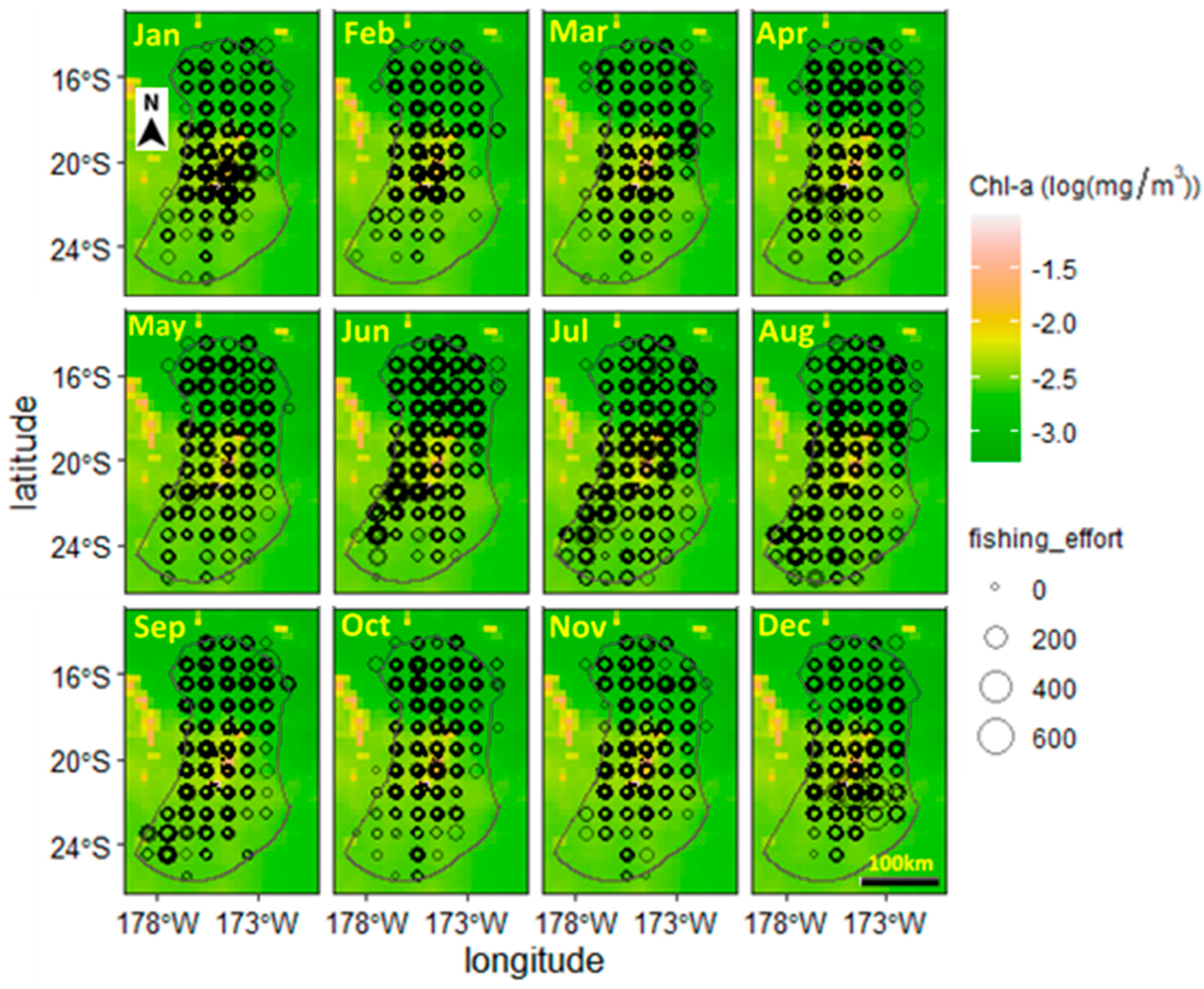
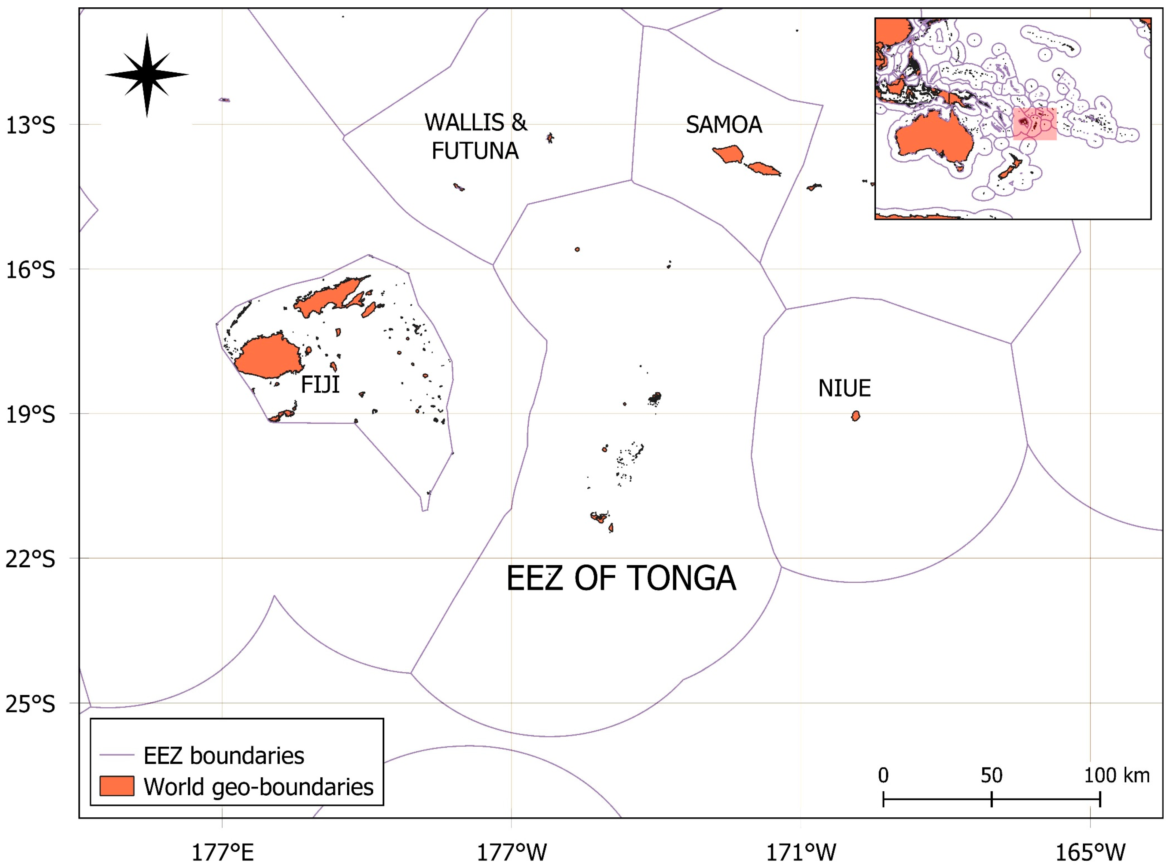
3.2. Spatial Distribution of Tuna Longliners

The monthly distributions of the spatial trajectory points of tuna longline vessels from 2002 to 2018 are shown in Figure 3. Based on the trajectory depicted, the area coverage by the vessels is from 171° to 179° W and from 14.5° to 25.5° S. The extent of the area occupied by vessels remained relatively constant throughout the months of the year. Starting in September, the concentrated area of vessels decreased and was mainly distributed near the central-northern area of the EEZ, with the lowest number of vessel locations in October and November. Starting in October, the area of vessels expanded in the central part of the EEZ and towards the north. The least concentrated area occupied by vessels is around 22°–25.5° S.

3.3. Model Training Results

This study considered the fishing effort of the tuna longline vessels as the dependent variable. After conducting a correlation analysis, nine environmental variables were obtained. DPT, depth, the spatial indices longitude and latitude, and the temporal indices month and year were also considered. A total of 15 independent variables were used for GAM modeling (Equation (1)). The training results are presented in Table S1. The average explained deviance of the training dataset is 48%, the average score of AUC is 0.57, the average training TPR score is 0.47, the TNR score is 0.72, and the overall training accuracy rate is 0.52. In this research, we used an identical dataset to train the BRT model, and the corresponding parameters are displayed in Table S2. The average explained deviance of the training dataset is 39%, the average score of AUC is 0.58, the average training TPR score is 0.45, the TNR score is 0.67, the TSS score is 0.12, and the overall training accuracy rate is 0.55

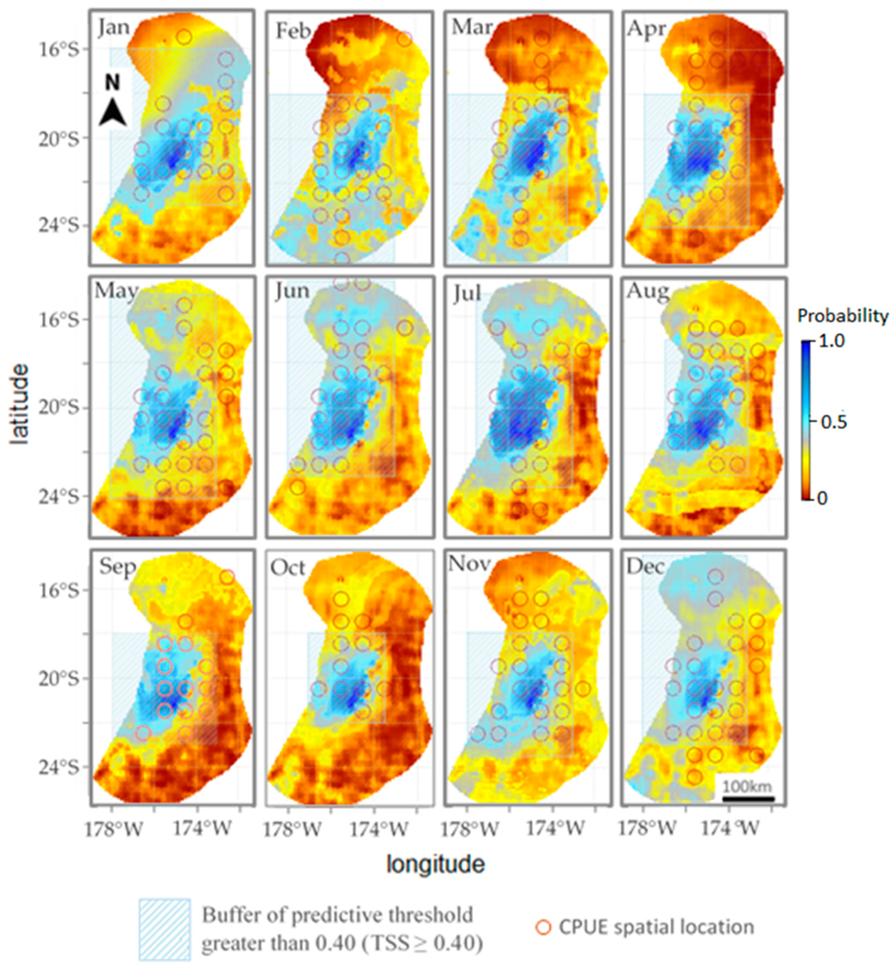
3.4. Prediction Accuracy of the Models

Figure 4 is a superimposed spatial map of the fishing effort predicted by the model in 2018 and the actual fishing effort spatial locations of fishing vessels in 2018. The image shows that each month has a good spatial distribution contrast indicated by actual fishing efforts that fall within the predictive threshold grid buffer (TSS ≥ 0.40). Based on the results of the two models (Tables S1 and S2), the BRT model was employed to evaluate the potential effects of the environmental factors on tuna longline fisheries. Our prediction results show an average AUC of 0.62, and the accuracy rate reaches 0.72. According to the space map from January to December, the areas with the largest amount of fishing effort predicted by vessels are concentrated at 173.5° W to 178° W and 18° S to 23.5° S. This is the area vessels focus their actual fishing efforts. The images from May to July show a second area, 16° S to 18° S, with a significant fishing effort being developed by the vessels, but it disappeared again in August. Beginning in March, the dense fishing effort zone grew more intense without expansion until August, and the fishing effort intensity decreased from September to December. The predictions show that July has the most fishing effort, while the months of November and December have the least. According to the forecasted fishing effort, there is no obvious trend except for the increase in fishing effort concentration from March to August and the decrease from September to December.

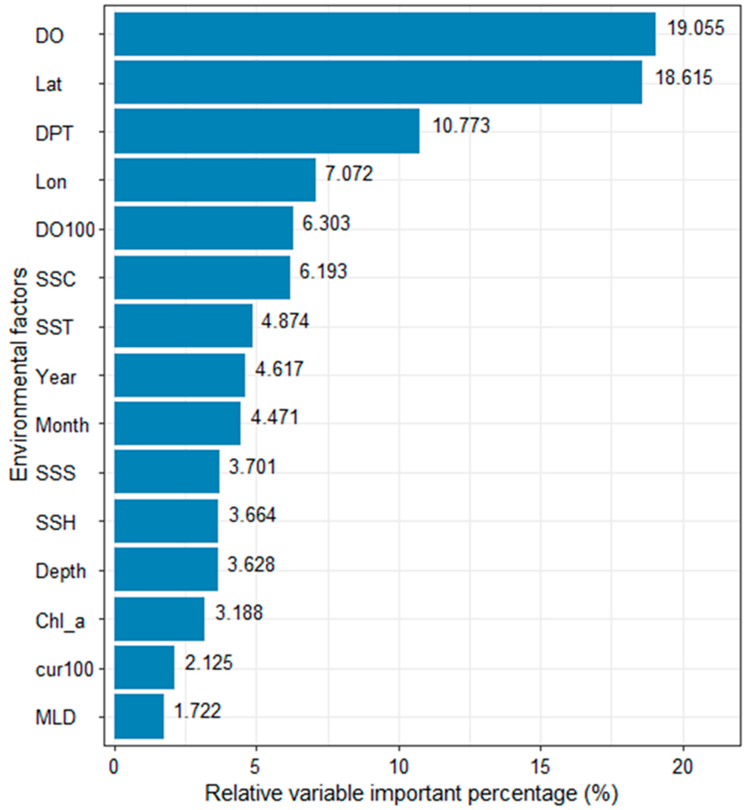
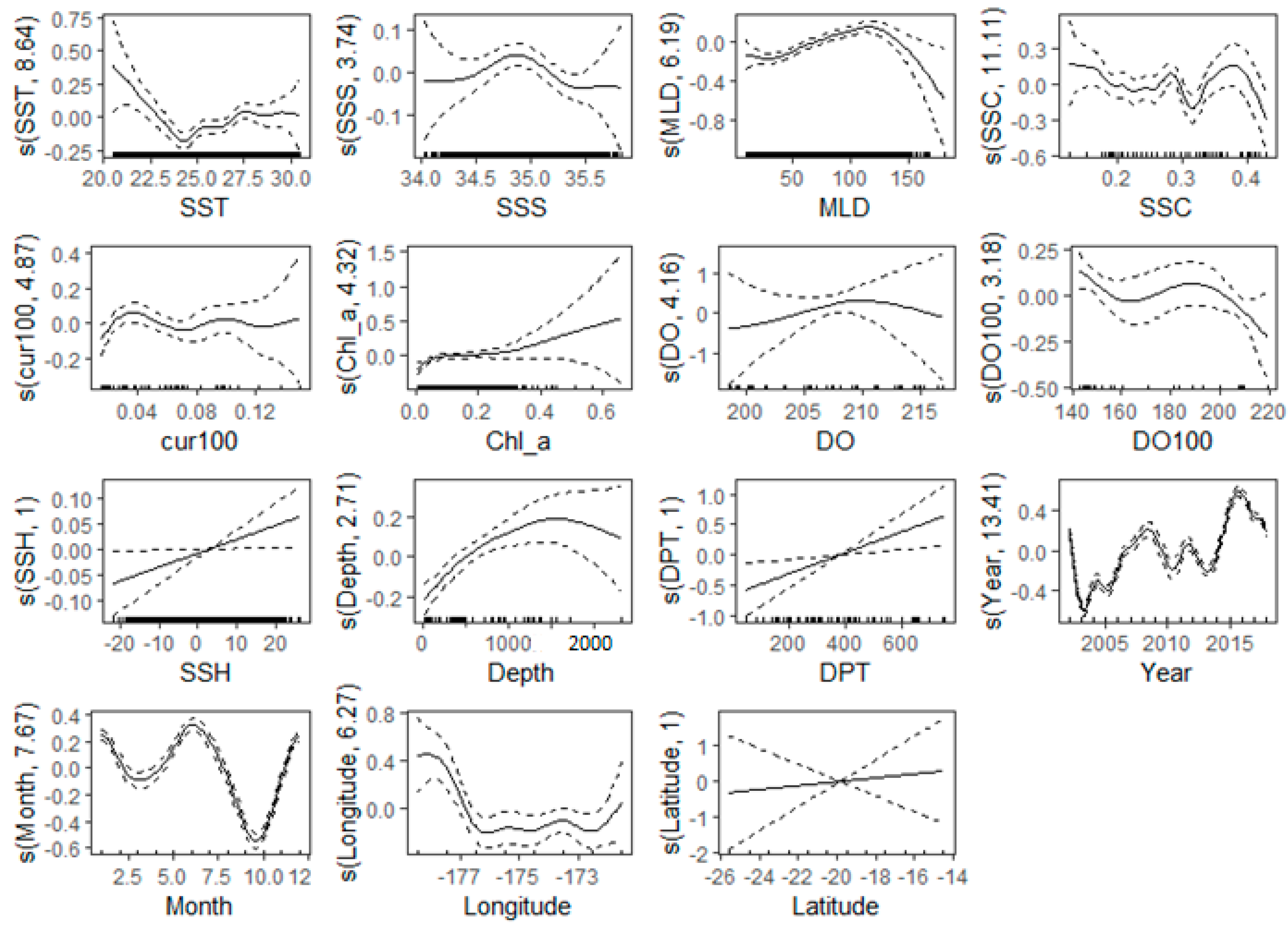
3.5. Contribution Rate of Environmental Factors

The average contribution rate of the selected variable value to the fishing effort of the vessel is shown in Figure 5. It can be seen from the bar chart as a whole that DO and latitude are the most important factors affecting the fishing effort of tuna longliners, and their contribution rates to the fishing effort of vessels are 19.06% and 18.62%, respectively. Second, DPT, longitude, DO100, and SSC have an effect on fishing effort of 10.77%, 7.07%, 6.30%, and 6.19%, respectively. SST, year, and month also have a certain influence, and their contribution rates are approximately 4%. The contribution rates of SSS, SSH, depth, and Chl-a are relatively small, approximately 3%. Cur100 and MLD show the lowest contribution rates of 2.13% and 1.72%, respectively.

Figure 6 illustrates the connection between crucial environmental factors and predictive factors spanning the years 2002 to 2018. The figure reflects the range of environmental factors corresponding to the most likely fishing effort and the specific contribution rate of environmental factors. DO and latitude are the most important variables and are mostly concentrated at 6.4–6.88 mgL⁻¹ and 18–22° S, respectively, with little fluctuation in their curves. The curves with the most fluctuations are year, month, SST, SSS, MLD, and SSC. For variable years, the minimum CPUE occurred in 2003, with a subsequent rise to its peak in 2016. During the months of the year, the CPUE is greater in winter (May–September) compared to summer months (October–March). In colder waters, specifically those with temperatures below 23.5 °C, a high CPUE was observed in relation to temperature. The highest fishing activity occurred in water, with a salinity range of 34.5 to 35.5 PSU. The MLD exhibits a gradual upward trend, commencing at 25 m and reaching its peak at 125 m. There was no significant fluctuation in water current concerning the fishing effort of vessels. Curves with the least fluctuations are cur100, Chl-a, and depth, which correspond to their small contributions in relative variable importance. Longitude was also among the first four important environmental variables, and the fishing effort of vessels is more concentrated in the 172–178° W region, and the contribution rate of longitude is relatively large.

4. Discussion

4.1. Environmental Factors and Vessel Data

Previous studies [65,66] have primarily focused on surface environmental factors in the context of longline tuna fishing. However, studies have indicated that bonito, yellowfin, and bigeye tuna are predominantly found and caught in the water column at depths ranging from 50 to 100 m below the surface [43,52]. Longline tuna fishing is predominantly conducted within the EEZ of a particular region, and the distance between the fishing vessel and the coastline can influence the available fishing opportunities. This study employs a set of 15 variables encompassing dynamic factors related to the ocean environment, spatial parameters, and static attributes like proximity to land, and it uses BRT and GAM models to elucidate how these various factors affect the geographical patterns of fishing operations.

Studies pertaining to tuna environmental habitats have been carried out in the past [24,25,26,27,28]. These investigations primarily used compiled fishery logbook data, integrating them with environmental parameters, to characterize the habitat of tuna. Therefore, compared with previous work, this study is consistent in using extracted fishing effort data of longline vessels as a predictor variable of the BRT and GAM models as a true and effective response to the behavior of the vessels. Hence, in contrast to earlier studies, this research maintains consistency by employing extracted fishing effort data from longline vessels as predictor variables in both the BRT and GAM models, as these accurately and effectively capture vessel behavior. The primary objective of a tuna longline vessel at sea is fishing, and with each period of time it remains on the water, it incurs a corresponding or additional cost. Hence, the examination of vessel fishing practices concerning fish habitats is crucial for the overall sustainability and vitality of the entire fishery.

4.2. The Model’s Goodness-of-Fit

In studies concerning the forecasting of marine environmental factors and the distribution of fishery resources, most researchers commonly employ models like the habitat suitability index (HSI) and support vector machine (SVM). However, the reliance on these models often results in overfitting, consequently diminishing the predictive accuracy of the model. Boosted regression trees (BRTs) represent a self-learning approach within ensemble learning based on the classification and regression tree algorithm, and they serve to mitigate the risk of overfitting in the model [61]. The boosted regression tree model was employed to examine the relationship between vessel fishing activities and environmental variables and to identify how vessel fishing behavior is influenced by environmental conditions based on environmental factors and fishing efforts [67]. As the number of training decision trees grows progressively, the boosted regression tree model’s fit to the training data improves. However, if the number of decision trees surpasses a specific threshold, it can lead to overfitting, causing a reduction in the model’s predictive accuracy. The GAM algorithm was employed due to its ability to capture complex and non-linear relationships within the fishery and environmental data [56]. Studies have shown that fishing effort is often influenced by factors such as environmental conditions, vessel characteristics, and temporal trends [50,52]. Furthermore, the flexibility of GAM allows it to accommodate these complexities and provide a more accurate representation of how environmental factors contribute to changes in fishing effort [53,54]. Our ensemble results exhibited and supported the corresponding nature of our environmental and fishery data, as shown in Figure 4 and Figure 6.

The results of all model training parameters confirm the accuracy of the model training. Through a comparison of the prediction parameters obtained from the GAM model (Table S1) and the BRT model (Table S2), a more suitable choice was made by opting for the BRT model for prediction. The BRT model forecasts the fishing effort of vessels in 2018, demonstrating greater alignment with the actual fishing effort observed in the spatial distribution region of that year. The model’s binary classification prediction accuracy reaches 55%, and both the training and prediction results have been verified.

4.3. Influence of Environmental Factors on Vessel Operations

The habitat of tuna is closely related to its oceanic environment [24,25,26,27,28,43,52]. Huang et al. (2020) [68] used latitude, longitude, mixed layer depth, month, and sea surface temperature and employed a second-order boosted regression tree model to construct a habitat model for free-swimming schools of bigeye tuna in the East Pacific, aiming to investigate its temporal and spatial distribution characteristics. Their findings indicated that latitude, longitude, mixed layer depth, month, and sea surface temperature are the primary factors influencing the success rate of bigeye tuna. The study by Nataniel et al. (2021) [69] showed that the capture potential of accumulating tuna biomass is linked to variables such as sea temperature, productivity, sea level height, and geostrophic flow, in addition to temporal and spatial factors. These findings align with several of the environmental variables considered in this article.

The shift in marine environmental conditions causes alterations in the distribution of fishery resources, therefore affecting how vessels track fish stocks. Consequently, modifications in vessel operating areas provide insights into alterations in the spatial distribution of fishery resources. The results in this paper show that DO and latitude are the most important factors affecting the fishing effort of tuna purse seiners. Second, DPT, longitude, DO100, SSC, and SST have the greatest impact on tuna longline fishing operations. The importance of DO, latitude, DPT, longitude, DO100, SSC, and SST totaled 72.80%, and seven variables contributed over 70% of the impact. These important results indicate that dissolved oxygen level in water, spatial factors, and the distance from the vessel to land are the key environmental variables that affect the operation of tuna longliners in the EEZ of Tonga.

The most substantial variable, accounting for 25.36% of the impact, was the oxygen content at both the sea surface and 100 m depth, which is particularly significant due to tuna’s demand for dissolved oxygen. Mallya (2007) reported a higher feeding rate of fish at higher oxygen saturation levels (between 80 and 120%) than at low oxygen saturation [70]. Wexler et al. (2011) [26] reported dissolved oxygen for survival, development, and growth of yellowfin tuna eggs and yolk-sac and first-feeding larvae more than 2.2 mgL⁻¹. Song and Zhou (2010) [71] reported water with dissolved oxygen less than 0.85 mgL⁻¹ had significant impacts on the spatial distribution of bigeye tuna. This study showed a dissolved oxygen level range between 6.4 and 6.88 mgL⁻¹, a notably substantial range when compared to the above studies, predictably holding the highest contribution rate among the variables in this research. Areas with lower dissolved oxygen concentrations may be less favorable for tuna, as they are often associated with reduced primary productivity and the availability of prey [26]. Changes in oxygen concentrations can affect the vertical and horizontal distribution of zooplankton and small fish, impacting the foraging behavior of tuna [68]. Different tuna species have varying tolerance levels for oxygen concentrations at different depths. Ocean deoxygenation, a consequence of climate change, has the potential to alter the distribution of tuna habitats [26,68].

Latitude and longitude have a high contribution rate, 18.61% and 7.07%, respectively, indicating that tuna longline operations are also spatially selective, and fishing vessels tend to operate in certain areas. Zhang et al. (2021) [52] discovered a concentrated clustering pattern in the fishing activities of tuna purse seiners within the WCPO. This clustering of fishing vessels in specific locations was associated with the target of their fishing activities. Yang et al. (2014) [72] observed a pronounced aggregation and distribution of bonito resources in the WCPO, along with a robust local spatial autocorrelation. This research shows that tuna longline fisheries operate mainly in latitude 18–22° S and longitude 172–178° W of the EEZ of Tonga. Latitude and longitude variation data allow fisheries managers to analyze the spatial distribution of tuna populations as different species of tuna have preferred temperature ranges, and their distribution is often correlated with specific oceanic conditions [63]. Understanding the geographical locations where tuna are most abundant helps in delineating fishing zones and optimizing fishing efforts [70]. By tracking latitude and longitude coordinates over time, fishery managers can gain insights into the seasonal movements of tuna stocks [70,73]. This information is critical for establishing appropriate time and area-based management measures.

The distance of longline vessels to land significantly influences the selection of fishing operations. Our partial dependence distribution map (Figure 6) shows that most fishing vessels operate 100–700 km from the main port in Nuku’alofa, indicating that longline vessels mostly operate within the EEZ of Tonga. Furthermore, considering vessel sizes in the small island nation, which range from 17.5 to 39.9 m [8], they tend to fish relatively close to ports, as the fishing distance is closely aligned with the vessel’s fuel capacity. Understanding the distance to the port is integral to effective tuna fishery management [71]. It influences operational efficiency, resource allocation, monitoring vessels’ time at sea and safety, and infrastructure development [62]. Incorporating this information into management strategies helps ensure the long-term sustainability and success of tuna fisheries [62,72].

Sea surface current and sea surface temperature also have a certain degree of influence on tuna longline fishing operations, while salinity, sea surface height, and bottom depth have little effect, and sea surface chlorophyll, water current at 100 m, and mixed layer depth have almost no effect on tuna longline fishing operations. Our results show tuna longline fishing appears more in areas where the sea surface temperature is between 22.5 and 30 °C; Tang et al. (2014) [74] showed a sea surface temperature range of 29–31 °C. Tuna are highly sensitive to water temperature, as it directly affects their metabolic rates, reproduction, and distribution [73]. Tuna, being warm-blooded, thrive in warmer waters, and their distribution is often correlated with temperature gradients [54]. Changes in ocean temperatures, influenced by phenomena like El Niño and La Niña, can result in shifts in tuna distribution patterns [43]. Warmer waters may lead to the expansion of certain tuna species into new areas, while colder temperatures can contract their range. Tuna management plans must be adaptive to these temperature fluctuations to anticipate shifts in migration and abundance [43,54,75].

5. Conclusions

This study integrated fishing effort data of tuna fisheries in Tonga with satellite-derived environmental data from 2002 to 2018 to analyze the behavior of tuna longline fishing effort using the BRT model and GAM model to construct the non-linear relationship between the spatial distribution of fishing effort and marine environmental factors. The partial effect plots of our BRT confirmed the non-linear relationships between the variables analyzed and tuna longline fishing operations. Among the 15 variables considered, DO, latitude, and DPT exhibited the highest contribution rate, followed by longitude and DO100. Our model prediction shows that a large amount of fishing effort is concentrated in 173.5° W to 178° W and 18° S to 23.5° S, which has a good spatial distribution contrast against the actual fishing efforts of tuna longline vessel operations. Overall, alterations in the marine environment exert a more significant influence on the distribution of tuna species, hence the spatial patterns of fishing vessel activities. Tuna longline fishing is aimed at locating fish stocks. The repercussions of these environmental factors on the operations of tuna longline fishing vessels can also shed light on their effects on the resources of the tuna longline fishery.

References

1. Krishnan, M.; Lakra, W.S. Coastal and Marine Fisheries Management in. Coast. Mar. Fish. Manag. SAARC Ctries. 2013, 196, 187. [Google Scholar]
2. Xu, K.; Feng, J.; Ma, X.; Wang, X.; Zhou, D.; Dai, Z. Identification of tuna species (Thunnini tribe) by PCR-RFLP analysis of mitochondrial DNA fragments. Food Agric. Immunol. 2016, 27, 301–313. [Google Scholar] [CrossRef]
3. Takeshima, H.; Yamaura, K.; Kuboshima, N.; Hiramatsu, M.; Kameya, C.; Nohara, K.; Sakuma, K.; Chiba, S.N.; Tawa, A.; Suzuki, N. A method for identifying nine tuna and tuna-like species (tribe Thunnini) by using high-resolution melting analysis based on genotyping single nucleotide polymorphisms in mitochondrial DNA. Conserv. Genet. Resour. 2023, 15, 153–159. [Google Scholar] [CrossRef]
4. WCPFC. Overview of Tuna Fisheries in the Western and Central Pacific Ocean, Including Economic Conditions; WCPFC-TCC13-IP0; Secretariat of the Pacific Community (SPC): Noumea, New Caledonia, 2010. [Google Scholar]
5. Barclay, K.; Cartwright, I. Governance of tuna industries: The key to economic viability and sustainability in the Western and Central Pacific Ocean. Mar. Policy 2007, 31, 348–358. [Google Scholar] [CrossRef]
6. Gillett, R.; McCoy, M.; Rodwell, L.; Tamate, J. Tuna: A Key Economic Resource in the Pacific Islands; A report prepared for the asian development bank and the forum fisheries agency; Asian Development Bank: Mandaluyong, Philippines, 2001; p. 108. [Google Scholar]
7. Bell, J.D.; Kronen, M.; Vunisea, A.; Nash, W.J.; Keeble, G.; Demmke, A.; Pontifex, S. Planning the use of fish for food security in the pacific. Mar. Policy 2009, 33, 64–76. [Google Scholar] [CrossRef]
8. MAFF; FFA. Tonga Tuna Fishery Framework 2018–2022; Ministry of Agriculture, Forestry; Fisheries, Fishery Forum Agency: Nuku’alofa, Tonga, 2018.
9. Collette, B.B.; Carpenter, K.E.; Polidoro, B.A.; Juan-Jordá, M.J.; Boustany, A.; Die, D.J.; Elfes, C.; Fox, W.; Graves, J.; Harrison, L.R.; et al. High value and long life—Double jeopardy for tunas and billfishes. Science 2011, 333, 291–292. [Google Scholar] [CrossRef] [PubMed]
10. Juan-Jordá, M.J.; Mosqueira, I.; Cooper, A.B.; Freire, J.; Dulvy, N.K. Global population trajectories of tunas and their relatives. Proc. Natl. Acad. Sci. USA 2011, 108, 20650–20655. [Google Scholar] [CrossRef] [PubMed]
11. Wright, G.; Rochette, J.; Gjerde, K.; Seeger, I. The Long and Winding Road: Negotiating a Treaty for the Conservation and Sustainable Use of Marine Biodiversity in Areas beyond National Jurisdiction; IDDRI: Paris, France, 2018. [Google Scholar]
12. Roy, A. Blue economy in the Indian Ocean: Governance perspectives for sustainable development in the region. ORF Occas. Pap. 2019, 181, 1–34. [Google Scholar]
13. Havice, E.; Campling, L. Shifting tides in the Western and Central Pacific Ocean tuna fishery: The political economy of regulation and industry responses. Glob. Environ. Politics 2010, 10, 89–114. [Google Scholar] [CrossRef]
14. Lan, K.-W.; Shimada, T.; Lee, M.A.; Su, N.J.; Chang, Y. Using remote-sensing environmental and fishery data to map potential yellowfin tuna habitats in the tropical pacific ocean. Remote Sens. 2017, 9, 444. [Google Scholar] [CrossRef]
15. Yen, K.W.; Lu, H.J.; Chang, Y.; Lee, M.A. Using remote-sensing data to detect habitat suitability for yellowfin tuna in the western and central pacific ocean. Int. J. Remote Sens. 2012, 33, 7507–7522. [Google Scholar] [CrossRef]
16. Mainuddin, M.; Saiton, K.; Saiton, S. Albacore fishing ground in relation to oceanographic conditions in the western north pacific ocean using remotely sensed satellite data. Fish. Oceanogr. 2008, 17, 61–73. [Google Scholar] [CrossRef]
17. Eveson, J.P.; Hobday, A.J.; Hartog, J.R.; Spillman, C.M.; Rough, K.M. Seasonal forecasting of tuna habitat in the Great Australian Bight. Fish. Res. 2015, 170, 39–49. [Google Scholar] [CrossRef]
18. Houssard, P.; Point, D.; Tremblay-Boyer, L.; Allain, V.; Pethybridge, H.; Masbou, J.; Ferriss, B.E.; Baya, P.A.; Lagane, C.; Menkes, C.E.; et al. A model of mercury distribution in tuna from the western and central Pacific Ocean: Influence of physiology, ecology and environmental factors. Environ. Sci. Technol. 2019, 53, 1422–1431. [Google Scholar] [CrossRef]
19. Wang, Y.; Liu, J.; Liu, H.; Lin, P.; Yuan, Y.; Chai, F. Seasonal and interannual variability in the sea surface temperature front in the eastern pacific ocean. J. Geophys. Res. Ocean. 2021, 126, e2020JC016356. [Google Scholar] [CrossRef]
20. Wiryawan, B.; Loneragan, N.; Mardhiah, U.; Kleinertz, S.; Wahyuningrum, P.I.; Pingkan, J.; Timur, P.S.; Duggan, D.; Yulianto, I. Catch per unit effort dynamic of yellowfin tuna related to sea surface temperature and chlorophyll in Southern Indonesia. Fishes 2020, 5, 28. [Google Scholar] [CrossRef]
21. Sambah, A.B.; Muamanah, A.; Harlyan, L.I.; Lelono, T.D.; Iranawati, F.; Sartimbul, A. Sea surface temperature and chlorophyll-a distribution from Himawari satellite and its relation to yellowfin tuna in the Indian Ocean. Aquac. Aquar. Conserv. Legis. 2021, 14, 897–909. [Google Scholar]
22. Hidayat, R.; Zainuddin, M.; Putri, A.R.S. Skipjack tuna (Katsuwonus pelamis) catches in relation to chlorophyll-a front in bone gulf during the southeast monsoon. Aquac. Aquar. Conserv. Legis. 2009, 12, 209–218. [Google Scholar]
23. Maravelias, C.D. Habitat selection and clustering of a pelagic fish: Effects of topography and bathymetry on species dynamics. Can. J. Fish. Aquat. Sci. 1999, 56, 437–450. [Google Scholar] [CrossRef]
24. Lumban-Gaol, J.; Leben, R.R.; Vignudelli, S.; Mahapatra, K.; Okada, Y.; Nababan, B.; Mei-Ling, M. Variability of satellite-derived sea surface height anomaly, and its relationship with bigeye tuna (Thunnus obesus) catch in the eastern indian ocean. Eur. J. Remote Sens. 2015, 48, 465–477. [Google Scholar] [CrossRef]
25. Teo, S.L.; Block, B.A. Comparative influence of ocean conditions on yellowfin and atlantic bluefin tuna catch from longlines in the gulf of mexico. PLoS ONE 2010, 5, e10756. [Google Scholar] [CrossRef] [PubMed]
26. Wexler, J.B.; Margulies, D.; Scholey, V.P. Temperature and dissolved oxygen requirements for survival of yellowfin tuna, Thunnus albacares, larvae. J. Exp. Mar. Biol. Ecol. 2011, 404, 63–72. [Google Scholar] [CrossRef]
27. Ganachaud, A.; Sen Gupta, A.; Brown, J.N.; Evans, K.; Maes, C.; Muir, L.C.; Graham, F.S. Projected changes in the tropical Pacific Ocean of importance to tuna fisheries. Clim. Chang. 2013, 119, 163–179. [Google Scholar] [CrossRef]
28. Cornic, M.; Rooker, J.R. Influence of oceanographic conditions on the distribution and abundance of blackfin tuna (Thunnus atlanticus) larvae in the Gulf of Mexico. Fish. Res. 2018, 201, 1–10. [Google Scholar] [CrossRef]
29. Reimer, M.N.; Abbott, J.K.; Wilen, J.E. Fisheries production: Management institutions, spatial choice, and the quest for policy invariance. Mar. Resour. Econ. 2017, 32, 143–168. [Google Scholar] [CrossRef]
30. Lacoursière-Roussel, A.; Côté, G.; Leclerc, V.; Bernatchez, L. Quantifying relative fish abundance with eDNA: A promising tool for fisheries management. J. Appl. Ecol. 2016, 53, 1148–1157. [Google Scholar] [CrossRef]
31. Crespo, G.O.; Dunn, D.C.; Reygondeau, G.; Boerder, K.; Worm, B.; Cheung, W.; Tittensor, D.P.; Halpin, P.N. The environmental niche of the global high seas pelagic longline fleet. Sci. Adv. 2018, 4, 3681. [Google Scholar] [CrossRef]
32. Juan-Jordá, M.J.; Murua, H.; Arrizabalaga, H.; Dulvy, N.K.; Restrepo, V. Report card on ecosystem-based fisheries management in tuna regional fisheries management organizations. Fish Fish. 2018, 19, 321–339. [Google Scholar] [CrossRef]
33. Crowder, L.; Norse, E. Essential ecological insights for marine ecosystem-based management and marine spatial planning. Mar. Policy 2008, 32, 772–778. [Google Scholar] [CrossRef]
34. Granek, E.F.; Polasky, S.; Kappel, C.V.; Reed, D.J.; Stoms, D.M.; Koch, E.W.; Kennedy, C.J.; Cramer, L.A.; Hacker, S.D.; Barbier, E.B.; et al. Ecosystem services as a common language for coastal ecosystem-based management. Conserv. Biol. 2010, 24, 207–216. [Google Scholar] [CrossRef]
35. Espinosa-Romero, M.J.; Chan, K.M.; McDaniels, T.; Dalmer, D.M. Structuring decision-making for ecosystem-based management. Mar. Policy 2011, 35, 575–583. [Google Scholar] [CrossRef]
36. Ochiewo, J. Changing fisheries practices and their socioeconomic implications in South Coast Kenya. Ocean. Coast. Manag. 2004, 47, 389–408. [Google Scholar] [CrossRef]
37. Eliasen, S.Q.; Papadopoulou, K.N.; Vassilopoulou, V.; Catchpole, T.L. Socio-economic and institutional incentives influencing fishers’ behaviour in relation to fishing practices and discard. ICES J. Mar. Sci. 2014, 71, 1298–1307. [Google Scholar] [CrossRef]
38. Su, F.; Zhou, C.; Lyne, V.; Du, Y.; Shi, W. A data-mining approach to determine the spatio-temporal relationship between environmental factors and fish distribution. Ecol. Model. 2004, 174, 421–431. [Google Scholar] [CrossRef]
39. Murray, G.; Neis, B.; Johnsen, J.P. Lessons learned from reconstructing interactions between local ecological knowledge, fisheries science, and fisheries management in the commercial fisheries of Newfoundland and Labrador, Canada. Hum. Ecol. 2006, 34, 549–571. [Google Scholar] [CrossRef]
40. Orben, R.A.; Adams, J.; Hester, M.; Shaffer, S.A.; Suryan, R.M.; Deguchi, T.; Ozaki, K.; Sato, F.; Young, L.C.; Clatterbuck, C.; et al. Across borders: External factors and prior behaviour influence North Pacific albatross associations with fishing vessels. J. Appl. Ecol. 2021, 58, 1272–1283. [Google Scholar] [CrossRef]
41. Hsu, T.Y.; Chang, Y.; Lee, M.A.; Wu, R.F.; Hsiao, S.C. Predicting skipjack tuna fishing grounds in the western and central Pacific Ocean based on high-spatial-temporal-resolution satellite data. Remote Sens. 2021, 13, 861. [Google Scholar] [CrossRef]
42. Wang, W.; Zhou, C.; Shao, Q.; Mulla, D. Remote sensing of sea surface temperature and chlorophyll-a: Implications for squid fisheries in the north-west pacific ocean. Int. J. Remote Sens. 2010, 31, 4515–4530. [Google Scholar] [CrossRef]
43. Arrizabalaga, H.; Dufour, F.; Kell, L.; Merino, G.; Ibaibarriaga, L.; Chust, G. Global habitat preferences of commercially valuable tuna. Deep Sea Res. Part II Top. Stud. Oceanogr. 2015, 113, 102–112. [Google Scholar] [CrossRef]
44. Zhou, W.F.; Chen, L.L.; Cui, X.S.; Zhang, H. Influence of Thermocline and Spatiotemporal Factors on the Distribution of Yellowfin Tuna Fishing Grounds in the Central and Western Pacific Under Abnormal Climate. China Agric. Sci. Technol. Rev. 2021, 23, 192–201. [Google Scholar]
45. Yang, S.L.; Shi, H.M.; Fan, X.M.; Cui, X.S.; Wang, F.; Zhang, H. Spatial Analysis of the Habitat of Yellowfin Tuna in the Tropical Central and Western Pacific. China Agric. Sci. Technol. Herald. 2022, 24, 183–191. [Google Scholar] [CrossRef]
46. Dell, J.; Wilcox, C.; Hobday, A.J. Estimation of yellowfin tuna (Thunnus albacares) habitat in waters adjacent to australia’s east coast: Making the most of commercial catch data. Fish. Oceanogr. 2011, 20, 383–396. [Google Scholar] [CrossRef]
47. Nicolas, B.; Walker, E.; Gaertner, D.; Rivoirard, J.; Gaspar, P. Fishing Activity of Tuna Purse Seinersestimated From Vessel Monitoring System (VMS) Data. Can. J. Fish. Aquat. Sci. 2011, 68, 1998–2010. [Google Scholar]
48. Zhang, C.L.; Jiang, Y.; Wang, B.Y.; Wang, D.Y.; Hu, S. Construction and Preliminary Analysis of the Vertical Temperature Structure of the Accompanying Fish School of Yellowfin Tuna in the Central and Western Pacific. J. Shanghai Ocean Univ. 2021, 33, 233–241. [Google Scholar]
49. Oyafuso, Z.S.; Drazen, J.C.; Moore, C.H.; Franklin, E.C. Habitat-based species distribution modelling of the Hawaiian deepwater snapper-grouper complex. Fish. Res. 2017, 195, 19–27. [Google Scholar] [CrossRef]
50. Stock, B.C.; Ward, E.J.; Eguchi, T.; Jannot, J.E.; Thorson, J.T.; Feist, B.E.; Semmens, B.X. Comparing predictions of fisheries bycatch using multiple spatiotemporal species distribution model frameworks. Can. J. Fish. Aquat. Sci. 2020, 77, 146–163. [Google Scholar] [CrossRef]
51. Vaihola, S.; Yemane, D.; Kininmonth, S. Spatiotemporal Patterns in the Distribution of Albacore, Bigeye, Skipjack, and Yellowfin Tuna Species within the Exclusive Economic Zones of Tonga for the Years 2002 to 2018. Diversity 2023, 15, 1091. [Google Scholar] [CrossRef]
52. Zhang, T.; Song, L.; Yuan, H.; Song, B.; Ebango Ngando, N. A comparative study on habitat models for adult bigeye tuna in the Indian Ocean based on gridded tuna longline fishery data. Fish. Oceanogr. 2021, 30, 584–607. [Google Scholar] [CrossRef]
53. Maunder, M.N.; Punt, A. Standardizing catch and effort data: A review of recent approaches. Fish. Res. 2004, 70, 141–159. [Google Scholar] [CrossRef]
54. Mugo, R.; Saitoh, S.I.; Nihira, A.; Kuroyama, T. Habitat characteristics of skipjack tuna (Katsuwonus pelamis) in the western North Pacific: A remote sensing perspective. Fish. Oceanogr. 2010, 19, 382–396. [Google Scholar] [CrossRef]
55. Martinez, L.A.; Harris, W.S.; Lee, D.Y. Assessing the importance of catch per unit effort in tuna distribution models for effective fisheries management. J. Ocean Fish. Stud. 2021, 37, 105–119. [Google Scholar]
56. Smith, J.R.; Johnson, M.K.; Thompson, P.Q. The role of catch per unit effort in modeling tuna distribution: Implications for sustainable fisheries management. Mar. Biol. Fish. Res. 2022, 54, 321–334. [Google Scholar]
57. Assis, J.; Tyberghein, L.; Bosch, S.; Verbruggen, H.; Serrão, E.A.; De Clerck, O.; Tittensor, D. Bio-ORACLE v2.0: Extending marine data layers for bioclimatic modelling. Glob. Ecol. Biogeogr. 2018, 27, 277–284. [Google Scholar] [CrossRef]
58. Lüdecke, D.; Ben-Shachar, M.S.; Patil, I.; Waggoner, P.; Makowski, D. performance: An R package for assessment, comparison and testing of statistical models. J. Open. Source Softw. 2021, 6, 3139. [Google Scholar] [CrossRef]
59. Naimi, B.; Hamm, N.; Groen, T.A.; Skidmore, A.K.; Toxopeus, A.G. Where is positional uncertainty a problem for species distribution modelling. Ecography 2014, 37, 191–203. [Google Scholar] [CrossRef]
60. R Development Core Team. R: A Language and Environment for Statistical Computing. Vienna, R Foundation for Statistical Computing. 2018. Available online: https://www.R-project.org/ (accessed on 9 April 2019).
61. Naimi, B.; Araújo, M.B. SDM: A reproducible and extensible r platform for species distribution modelling. Ecography 2016, 39, 368–375. [Google Scholar] [CrossRef]
62. Stramma, L.; Prince, E.D.; Schmidtko, S.; Luo, J.; Hoolihan, J.P.; Visbeck, M.; Wallace, D.W.; Brandt, P.; Körtzinger, A. Expansion of oxygen minimum zones may reduce available habitat for tropical pelagic fishes. Nat. Clim. Chang. 2012, 2, 33–37. [Google Scholar] [CrossRef]
63. Tidd, A.N.; Hutton, T.; Kell, L.T.; Blanchard, J.L. Dynamic prediction of effort reallocation in mixed fisheries. Fish. Res. 2012, 125, 243–253. [Google Scholar] [CrossRef]
64. Stevenson, T.C.; Tissot, B.N.; Walsh, W.J. Socioeconomic consequences of fishing displacement from marine protected areas in Hawaii. Biol. Conserv. 2013, 160, 50–58. [Google Scholar] [CrossRef]
65. Setiawati, M.D.; Sambah, A.B.; Miura, F.; Tanaka, T.; As-syakur, A.R. Characterization of bigeye tuna habitat in the Southern Waters off Java–Bali using remote sensing data. Adv. Space Res. 2015, 55, 732–746. [Google Scholar] [CrossRef]
66. Tseng, C.T.; Sun, C.L.; Yeh, S.Z.; Chen, S.C.; Su, W.C. Spatio-temporal distributions of tuna species and potential habitats in the Western and Central Pacific Ocean derived from multi-satellite data. Int. J. Remote Sens. 2010, 31, 4543–4558. [Google Scholar] [CrossRef]
67. Megan, A.C.; Anderson, M.; Schramek, T.; Merrifield, S.; Terrill, E.J. Towards a Fishing Pressure Prediction System for a Western Pacific EEZ. Sci. Rep. 2019, 9, 461–470. [Google Scholar]
68. Huang, J.L.; Dai, L.B.; Wang, X.F.; Zhou, C.; Tang, H. Spatial and Temporal Distribution Characteristics of Habitat Preference of Free-Swarming Tuna in the Eastern Pacific Ocean. J. Shanghai Ocean Univ. 2020, 29, 889–898. [Google Scholar]
69. Nataniel, A.; Lopez, J.; Soto, M. Modelling Seasonal Environmental Preferences of Tropical Tuna Purse Seine Fisheries in the Mozambique Channel. Fish. Res. 2021, 243, 106073. [Google Scholar] [CrossRef]
70. Mallya, Y.J. The effects of dissolved oxygen on fish growth in aquaculture. In The United Nations University Fisheries Training Programme, Final Project; United Nations University: Reykjavik, Iceland, 2007. [Google Scholar]
71. Song, L.; Zhou, Y. Developing an integrated habitat index for bigeye tuna (Thunnus obesus) in the Indian Ocean based on longline fisheries data. Fish. Res. 2010, 105, 63–74. [Google Scholar] [CrossRef]
72. Yang, X.M.; Dai, X.J.; Tian, S.Q.; Zhu, G.P. Hot Spot Analysis and Spatial Heterogeneity of Bonito Purse Seine Fishery Resources in the Central and Western Pacific. Chin. J. Ecol. 2014, 34, 3771–3778. [Google Scholar]
73. Stoner, A.W. Effects of environmental variables on fish feeding ecology: Implications for the performance of baited fishing gear and stock assessment. J. Fish. Biol. 2004, 65, 1445–1471. [Google Scholar] [CrossRef]
74. Tang, F.H.; Cui, X.S.; Yang, S.L.; Zhou, W.F.; Cheng, T.F.; Wu, Z.L. GIS Spatiotemporal Analysis of the Impact of Marine Environment on the Western and Central Pacific Ocean Tuna Purse Seine Fishing Grounds. South. Fish. Sci. 2014, 10, 18–26. [Google Scholar]
75. Putri, A.R.S.; Zainuddin, M.; Musbir, M.; Mustapha, M.A.; Hidayat, R.; Putri, R.S. Impact of increasing sea surface temperature on skipjack tuna habitat in the Flores Sea, Indonesia. IOP Conf. Ser. Earth Environ. Sci. 2021, 763, 012012. [Google Scholar] [CrossRef]
Figure 1. Map of the study area highlighting the EEZ, longitude 14.5° S–20.22° S, longitude 171.31° W–179.10° W, of Tonga, situated in the South Pacific region.
Fishes 08 00602 g001
Figure 2. The relationship of the fishing effort of vessels in relation to the number of fishing vessels during the years 2002–2018.
Fishes 08 00602 g002
Figure 3. An image showing the spatial distribution of the mean fishing effort of tuna longline vessels within the EEZ, longitude 14.5° S–20.22° S, longitude 171.31° W–179.10° W, of Tonga. Circles with thicker borders are due to the multiple years, 2002–2018, of data being plotted on top of each other.
Fishes 08 00602 g003
Figure 4. The predictive probability map of the fishing effort overlaid over single actual fishing effort (red solid circles) spatial locations of fishing vessels in the year 2018. Also shown is the buffer (in light green shaded area) of the predictive threshold greater than 0.40 to illustrate the good spatial distribution contrast between predicted fishing effort and the actual fishing effort.
Fishes 08 00602 g004
Figure 5. The average contribution rate in percentage of variables to fishing efforts of vessels in the EEZ, longitude 14.5° S–20.22° S, longitude 171.31° W–179.10° W, of Tonga in the years 2002–2018.
Fishes 08 00602 g005
Figure 6. Partial dependence plots showing the relationship between the environmental changes and CPUE of longline vessels for the years 2002–2018.
Fishes 08 00602 g006