Modeling Discards in Stock Assessments: Red Grouper Epinephelus morio in the U.S. Gulf of Mexico

Abstract

To be as accurate as possible, stock assessments should account for discard mortality in fisheries if it occurs. Three common approaches to modeling discards in assessments are to lump dead discards with landings, treat dead discards as their own fleet, or link them conversely with landings through use of a retention function. The first approach (lumping) implicitly assumes that the selectivity of landings applies also to discards. In many cases, that assumption is false, for example, if discards comprise smaller fish than do landings. The latter two approaches avoid the assumption by modeling discards explicitly with their own selectivity pattern. Here, we examine these approaches to modeling discards. Using a simulation study, we demonstrate that the two approaches to modeling discards explicitly can provide identical results under both static and time-varying conditions. Then, using a stock assessment case study of red grouper Epinephelus morio in the U.S. Gulf of Mexico, we demonstrate that in practice the approaches to modeling discards can provide different outcomes, with implications for the resultant management advice. We conclude by comparing and contrasting the different approaches, calling for more research to elucidate which approach is most suitable under various sources of error typically encountered in discard data.

1. Introduction

Fishery bycatch is recognized worldwide as a critical issue in marine conservation and resource management [1]. Much of this unintentional or non-targeted portion of the catch is returned to sea, and these discards can have high release mortality rates depending on factors such as morphology, fishing gear, environmental conditions, and depth of capture [2,3]. Consequently, discarding has been considered as wasteful of natural resources [4,5,6], having effects on fish populations and marine ecosystems [7,8,9].

Globally, discards comprise nearly 10% of total catch [6,10]. In the United States (U.S.), discards comprise approximately 22% of total catch and, in the Southeast United States, that value is as high as 37% [5]. Similarly high discard percentages have been reported in the North Sea [11] and western North Atlantic [12]. To reduce discarded bycatch, resource managers have predominately relied on market forces, reductions in fishing effort, spatiotemporal fishing restrictions, and gear modifications [5]. More sweepingly, the European Union has recently legislated a discard ban (a.k.a., landing obligation) on quota-managed species [13,14].

Discarding occurs for a host of interacting reasons [15,16]. Some regulatory measures, such as size or bag limits, sex-specific restrictions (e.g., male-only harvest), and seasonal closures or quotas, mandate that animals be returned to the water when their harvest is prohibited. Quota programs, such as the red snapper Lutjanus campechanus and grouper-tilefish individual fishing quota (IFQ) programs, were implemented in the U.S. Gulf of Mexico (hereafter referred to as the Gulf) to increase harvesting efficiency (i.e., reduce discards), but such programs can lead to the discarding of legal-sized fish in the absence of quota. Market conditions may create economic incentives for discarding, including high-grading [17,18,19] or landing of plate-sized fish [20]. Discards in mixed-stock fisheries can be affected by the catch composition [21]. Whether discards are driven by species composition, year-class strength, fishing regulations, on-board constraints of gear or processing, market incentives, depredation, fisher preferences (e.g., targeting larger fish for retention [22]), or the interactions of multiple drivers, the underlying mechanisms result in a process that is dynamic in both time and space [11,16,19,23].

Some stock assessments ignore discards, particularly in cases when release mortality is considered negligible or when data on discards are sparse or unavailable. Otherwise, there is general consensus on the importance of including discards in assessments to characterize total removals accurately [24,25,26,27]. Discard mortalities are generally included in stock assessments by lumping them with landings or by modeling them explicitly. Lumping with landings may be a practical approach for its relative simplicity; however, a tacit assumption is that selectivity of discards equals that of landings. In many cases, such an assumption is unjustified if discards and landings comprise different sizes or ages of fish. For example, a size limit would typically result in discarded fish that are smaller and younger than landed fish. Modeling discards explicitly allows for differences in the selectivity of discard mortalities and landings.

The two most common approaches to model discards explicitly are either to apply a retention function or to include a discards-as-fleet component. The retention-function approach estimates total catch at age (or length) and then apportions that catch into landings or discards based on retention at age (or length) [21,25]. The fishing effort directed toward landings also applies to discards, such that a single fishing rate can be allocated to each component of removals. The discards-as-fleet approach (hereafter, the separate-fleet model) treats discard mortality as stemming from its own fleet, allowing for the fishing rates toward discards to be distinct from the fishing rates toward landings. Thus, a benefit of the separate-fleet approach is its flexibility, but at the cost of increased dimensionality, i.e., double the number of (typically annual) fishing mortality rates. It is possible to relax the assumption of static allocation with the retention-function approach; however, the additional parameters required for time-varying allocation increases dimensionality, equaling that of the separate-fleet model for annual allocations.

Here, we focus on the retention-function and separate-fleet approaches to modeling discards in stock assessments. We describe the two approaches mathematically, and we configure a simulation model of population and fishery dynamics to illustrate that the two approaches can provide identical results under both static and time-varying allocation. Using a case study, we demonstrate how these different approaches affect an assessment of Gulf red grouper Epinephelus morio and the resultant management advice.

2. Materials and Methods

2.1. Description of Discard Models and Simulations

Section 2.1 details simulations utilizing age-structured population and fishery dynamics, as well as the retention-function and separate-fleet approaches to modeling discards. The equations are standard in common stock assessment packages, such as Stock Synthesis [28].

2.1.1. Population and Fishery Dynamics

To demonstrate application of the two discard modeling approaches, we simulated population and fishery dynamics under multiple assumptions about fishing effort. For both approaches, abundance (N) of age (a) in year (t) was modeled with exponential decay,

$$N_{a+1,t+1}=N_{a,t}{e}^{-Z_{a,t}}$$

(1)

where $Z_{a,t}$ is total mortality rate of age a fish in year t, the sum of age-invariant natural mortality (M) and fishing rate ($F_{a,t}$). We modeled ages 1–12, with the oldest age A = 12 being an accumulator class (plus group).

Recruits (age-1 fish) were modeled assuming lognormal variation,

$$N_{1,t}=R{e}^{{\epsilon }_t} \mathrm{for} t> 1$$

(2)

where R is expected recruitment in the absence of noise and ${\epsilon }_t~N\left(0,{\sigma }_R\right)$. Initial (t = 1) abundance at age was computed given initial recruitment $N_{1,1}=R$ and equilibrium age structure for ages 2+ conditional on $Z_{a,1}$.

2.1.2. Retention-Function Approach

Under the retention-function approach, total catch is computed and then apportioned into landings and discards according to a retention ogive. We modeled selectivity of the catch as an age-based logistic function,

$$S_a^C=1/\left(1+e^{-{\beta }_1\left(a-{\alpha }_1\right)}\right)$$

(3)

where ${\beta }_1$ defines the slope and ${\alpha }_1$ defines the age at 50% selection. Similarly, the retention ogive followed a logistic function,

$$S_a^R=p/\left(1+e^{-{\beta }_2\left(a-{\alpha }_2\right)}\right)$$

(4)

where ${\beta }_2$ defines the slope, ${\alpha }_2$ defines the age at 50% retention, and p defines the asymptotic retention that can range $\left[0,1\right]$. A value of p < 1 indicates that discards include older fish, as may be the case under regulations such as closed seasons, bag limits, or trip limits. Combining catch and retention, selectivity of landings is the product,

$$S_a^L=S_a^C{S}_a^R$$

(5)

and selectivity of discards is,

$$S_a^D=S_a^C\left(1-S_a^R\right)$$

(6)

then, given a total annual fishing rate (${\mathcal{F}}_t$) and release mortality rate ($\delta$), annual fishing mortality at age for the retention model is computed,

$$F_{a,t}=\left(S_a^L+\delta S_a^D\right){\mathcal{F}}_t$$

(7)

2.1.3. Separate-Fleet Approach

Under the separate-fleet model, fishing rates for landings and discards are quantified as distinct from each other, as are selectivity functions. Annual fishing mortality at age is the sum,

$$F_{a,t}=S_a^L{F}_t^L+S_a^D{F}_t^D$$

(8)

where $F_t^L$ is the annual fishing rate toward landings and $F_t^D$ is the annual fishing rate toward discard mortalities. For application, a stock assessment model would estimate $F_t^D$ by fitting to a time series of dead discards (i.e., annual total discards multiplied by the release mortality rate), no different from how it would estimate $F_t^L$ by fitting to a time series of retained catch. Because the separate fleets are not linked by a retention function, there exists no underlying assumption about static allocation between landings and discards. In practice, the two modeling approaches would deviate in their predictions if selectivity functions were formulated differently. However, for the purpose of demonstrating that the two models can produce identical results, we assumed in our simulations that selectivity functions ($S_a^L$ and $S_a^D$) were the same for the separate-fleet and retention models.

2.1.4. Simulation Scenarios

Using the two modeling approaches, we simulated population and fishery dynamics under four different scenarios, each for 20 years. For the retention-function approach, we generated total annual fishing rates in all scenarios assuming lognormal variation,

$${\mathcal{F}}_t=\overline{\mathcal{F}}{e}^{{\gamma }_t}$$

(9)

where $\overline{\mathcal{F}}$ is the base-level rate in the absence of noise and ${\gamma }_t~N\left(0,{\sigma }_F\right)$. For the separate-fleet model, we assumed $F_t^L={\mathcal{F}}_t$ and $F_t^D=\delta {\mathcal{F}}_t$.

The four simulation scenarios differed in their assumptions about retention. Simulation 1 assumed static retention for all 20 years. Simulation 2 assumed a block structure, in which retention shifted toward older, larger fish in the second half of the simulation. This structure mimics implementation of a size limit. Simulation 3 assumed a trend in asymptotic retention, increasing linearly over the 20 years from p = 0.5 to p = 1.0. This structure mimics an increase over time in desirability, for example, as a market develops for that species. Simulation 4 combines the block structure of Simulation 2 with time-varying asymptotic retention; however, rather than a linear trend, asymptotic retention varies randomly each year drawn from a uniform distribution, $p~U\left(0.5,1.0\right)$. Although we consider these simulated patterns in selectivity to be somewhat arbitrary, the intent is not a comprehensive simulation study, but simply to demonstrate that predicted dynamics under the two approaches can match identically.

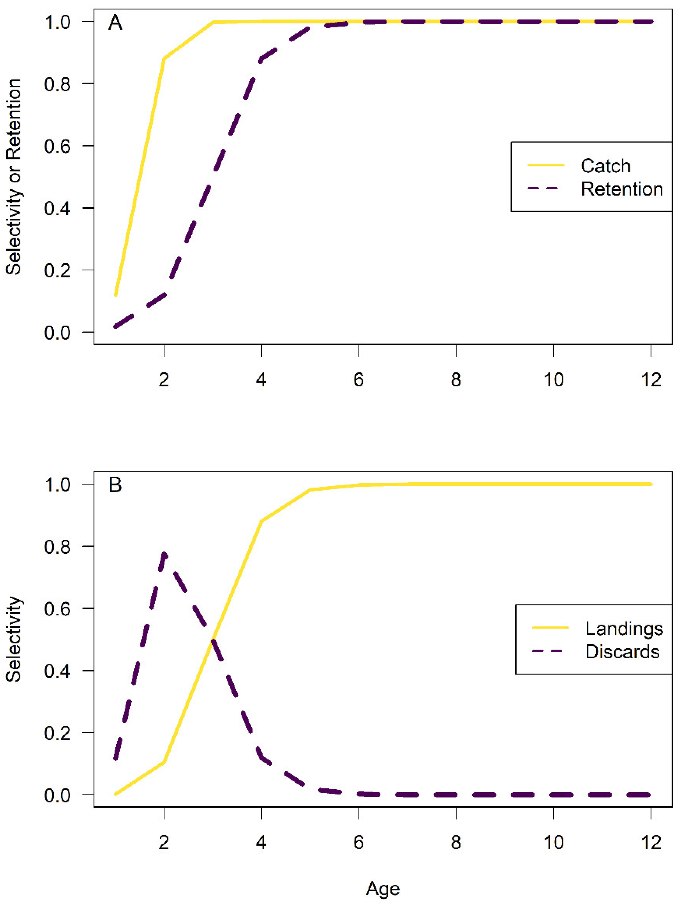
The parameter values used in our simulations were not based on any particular stock (

Table 1. Parameters of simulation models.

Parameter	Description	Value
General
M	Natural mortality rate	0.2
R	Expected recruitment in the absence of deviations	1e6
${\sigma }_R$	Standard deviation of recruitment deviations (log space)	0.5
δ	Release mortality rate	0.25
${\beta }_1$	Slope parameter of catch selectivity	4.0
${\alpha }_1$	Location parameter of catch selectivity	1.5
$\overline{\mathcal{F}}$	Base-level fishing rate	0.3
${\sigma }_F$	Standard deviation of fishing rate deviations (log space)	0.2
Simulation 1
${\beta }_2$	Slope parameter of retention function	2.0
${\alpha }_2$	Location parameter of retention function	3.0
p	Asymptotic retention	1.0
Simulation 2
${\beta }_2$	Slope parameter of retention function, years 1–10	2.0
${\alpha }_2$	Location parameter of retention function, years 1–10	3.0
${\beta }_2$	Slope parameter of retention function, years 11–20	4.0
${\alpha }_2$	Location parameter of retention function, years 11–20	5.0
p	Asymptotic retention	1.0
Simulation 3
${\beta }_2$	Slope parameter of retention function	2.0
${\alpha }_2$	Location parameter of retention function	3.0
p	Asymptotic retention, increases linearly over years	(0.5, …, 1.0)
Simulation 4
${\beta }_2$	Slope parameter of retention function, years 1–10	2.0
${\alpha }_2$	Location parameter of retention function, years 1–10	3.0
${\beta }_2$	Slope parameter of retention function, years 11–20	4.0
${\alpha }_2$	Location parameter of retention function, years 11–20	5.0
p	Asymptotic retention, varies randomly over years	p~U (0.5, 1.0)

), and we note that the generality of results does not depend on the specific values. For Simulation 1, the values of selectivity parameters defined catch selectivity that peaked at age 3 and retention that peaked at age 6 (Figure 1A), resulting in dome-shaped selectivity of discards and asymptotic selectivity of landings (Figure 1B). Variations on that pattern for Simulations 2–4 are as described above. All simulations were coded in R [29].

2.2. Case Study: Gulf Red Grouper

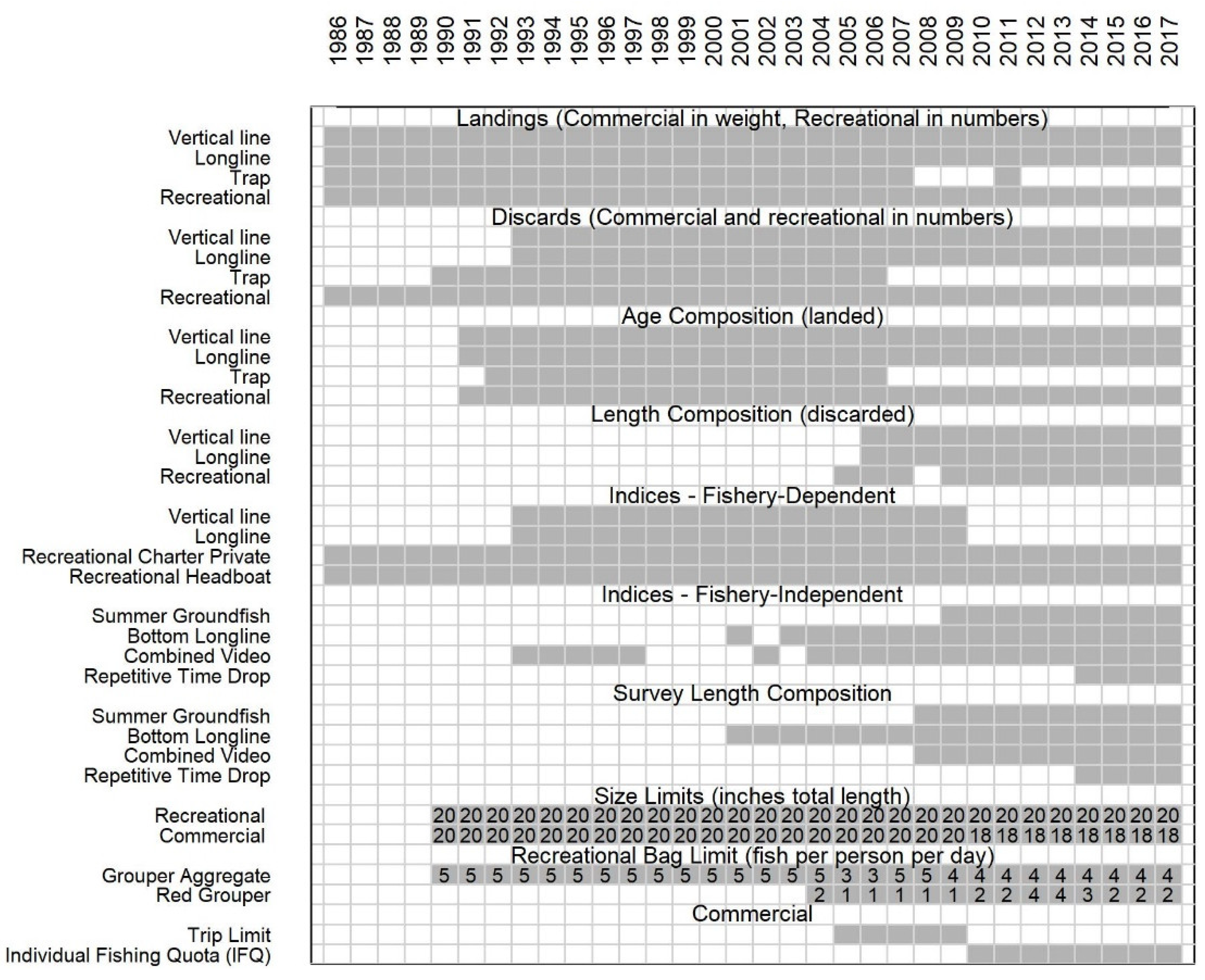
We considered the stock assessment of Gulf red grouper as a case study to demonstrate the different approaches to incorporating discards and to explore any differences in assessment outcome. The 2019 Gulf red grouper stock assessment was conducted using an age-structured, integrated model that utilized the retention-function approach for discards within Stock Synthesis 3.30.13 [28,30]. The base model consisted of a single area and covered the years 1986–2017, with the population initialized in a fished condition. The assessment included three commercial fleets (vertical line, longline, and trap) and one recreational fleet, with associated data inputs including landings, discards, indices of abundance (catch-per-unit-effort), age compositions of landed fish, and length compositions of discarded fish where available (Figure 2). The base model additionally included red tide as a source of mortality, which was estimated within the stock assessment for years (2005, 2014) of severe red tide blooms [31]. Relative abundance data and length compositions described adult red grouper from three fishery independent surveys (bottom longline, video, and repetitive timed drop of vertical line gear) and juveniles from one fishery independent survey (groundfish trawl). Length compositions of discarded fish were obtained from both the National Marine Fisheries Service (NMFS) Reef Fish Observer Program [32] and the Florida Fish and Wildlife Conservation Commission’s Fish and Wildlife Research Institute (FWRI) At-Sea Observer Program [33,34], which allowed for the estimation of time-varying retention patterns for the commercial vertical line and longline and recreational fleets. Uncertainty in parameter estimates and derived quantities were computed by Stock Synthesis based on asymptotic standard errors. Although these measures likely underrepresent the true uncertainty, asymptotic estimates of standard errors are ready output of most stock assessment models and are therefore commonly reported. Additional details on the base model can be found in the assessment report [35].

The Gulf red grouper fishery has experienced changes in management regulations over time for both the commercial and recreational sectors (Figure 2). The most significant change was the implementation of the Grouper-Tilefish Individual Fishing Quota Program in the commercial sector in 2010, which drastically changed fishing behavior and strived to reduce discards and the race to fish [36]. In the stock assessment model, these management changes were linked to retention rather than selectivity, with the latter assumed constant over time for each fishing fleet.

2.2.1. Base Model Configuration

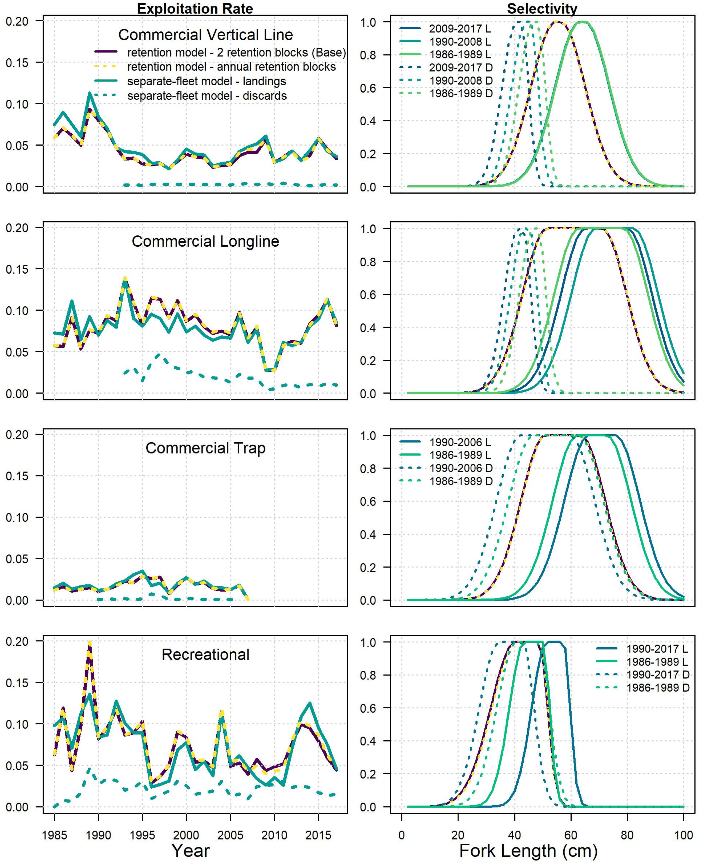
In the base model, all fish caught prior to the implementation of management regulations were assumed to be retained. Time-varying retention following a logistic function was implemented via time blocks to account for changes in size limits and the implementation of the commercial IFQ program (Figure 2). For each fishing fleet, the inflection point of the retention pattern was fixed at each time period’s respective size limit. Full retention (i.e., 100% retention) was assumed above the size limit for the commercial fleets for parsimony in the base model, whereas the asymptote parameter was estimated for the recreational fleet to allow for less than 100% retention due to bag limits and other restrictions. The slope of the retention function for each fleet was generally estimated within the base model where discard length data allowed, with the exception of the 1990–2008 time period for the commercial vertical line and the 1990–2017 time period for the recreational fleet. The slopes for these two situations were fixed in the base model after examining output diagnostics (e.g., high correlations with other parameters and jitter analysis [35]).

The base model estimated total discards based on the selectivity and retention functions, then calculated (and fit) dead discards (in numbers) based on the release mortality rate. Fleet-specific release mortality rates were treated as fixed model inputs for the commercial vertical line (19%), the commercial longline (41.5%), the commercial trap (10%), and the recreational fleet (11.6%). Dead discards were fitted assuming a lognormal error structure and a CV of 29% (derived from expert opinion) for each fishing fleet.

2.2.2. Alternative Model Configurations

For this study, we developed two alternative Gulf red grouper models to explore different approaches for incorporating discards and compared their results to the base model (also referred to as “retention model—2 blocks”). The first alternative was identical to the base model except that both the slope and asymptote parameters of the retention curves were estimated annually for each fleet where discard length composition was available (model referred to as “retention model—annual blocks”). The second alternative treated dead discards as landings in a separate fleet (model referred to as “separate-fleet model”), with the model configuration kept as similar to the base model as possible. This alternative required a few modifications for modeling selectivity, including (1) allowing two time blocks and estimating the peaks to mimic the block treatment for retention due to changes in size limits; (2) estimating the descending and ascending limb of the size-selectivity curves for the commercial vertical line and longline discard fishing fleets; (3) removing the priors on commercial longline size selectivity parameters for the top logit and descending limb (priors initially included in the base to improve stability); (4) fixing the length at the minimum age at the base model estimate (to avoid bounding at the low end); and (5) starting commercial discards in 1993 (rather than 1990) when observations began. This configuration also required additional parameters to estimate annual fishing mortality for each discard fleet. We refit each model and reran equilibrium projections aimed at achieving an F_MSY proxy of 30% spawning potential ratio, to evaluate the effect of model configuration on the assessment outcome. The projections extended 100 years and assumed recent fishing practices of selectivity and discarding would persist, as would the current allocation of 76% commercial landings and 24% recreational landings (by weight). Stock status metrics were then obtained by comparing the estimates of spawning stock biomass (SSB) and fishing mortality rate (F) from the terminal year of the projection to the analogous metrics from the terminal year of the assessment.

3. Results

3.1. Simulation Examples

Because of similarities in results across simulation examples, we show full outcomes here only for Scenario 1, in which retention was static (Figure 3). In that scenario, the fishing rates toward landings and toward discards fluctuated around their mean values (Figure 3A,B), as configured. Recruitment did the same, but with its largest and smallest values occurring near the end of the time series (Figure 3C). These stochastic events in recruitment subsequently carried through into abundance (Figure 3D), dead discards (Figure 3E), and landings (Figure 3F). The key result was that fishery and population dynamics were identical for the two approaches to modeling discards.

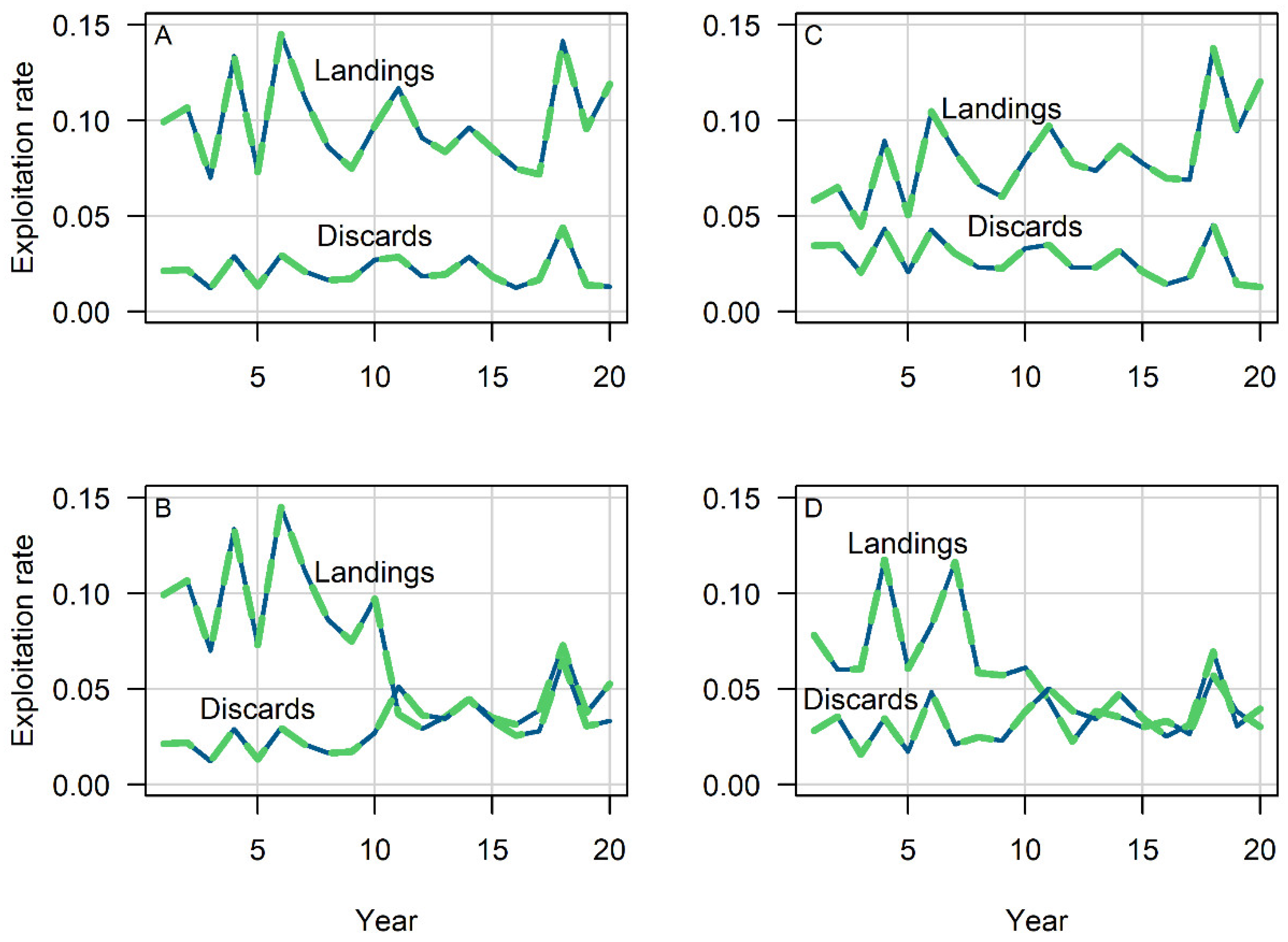
Although specific patterns were not the same across scenarios, in all cases the retention-function and separate-fleet approaches provided identical dynamics. This result can be seen by examining exploitation rates associated with landings (i.e., landings divided by abundance) and with discard mortalities (i.e., dead discards divided by abundance). In Scenario 1, exploitation rates fluctuated around their mean values (Figure 4A). Scenario 2 showed a shift in exploitation rates when the simulated size limit took effect; in the first half of the time series, exploitation rates associated with landings were substantially higher than those of discards, but in the second half, the two rates were nearly equal (Figure 4B). Scenario 3 showed a steady divergence in exploitation rates as retention increased (Figure 4C). The pattern in Scenario 4 was similar to that of Scenario 2, but the annual fluctuation in asymptotic retention resulted in a less pronounced difference between exploitation rates in the first half of the time series (Figure 4D). Again, the key result across all simulations was that the retention-function and separate-fleet approaches provided identical results.

3.2. Gulf Red Grouper Case Study

3.2.1. Comparison of Derived Quantities

Both the separate-fleet model and the base model re-parameterized to allow annual retention blocks had considerably more estimated parameters than the base model, which led to higher overall maximum gradients and a greater number of parameters with CVs exceeding 1 (

Table 2. Comparison of model results for the Gulf red grouper case study exploring different approaches to modeling discards. Note that negative log likelihoods are not comparable for the separate-fleet model due to changes in input data.

Main Change	Retention Model— 2 Blocks (Base)	Retention Model— Annual Blocks	Separate-Fleet Model
Model Evaluation
Negative log likelihood (NLL)	537.486	544.787	536.053
Catch NLL	36.5	34.5	3.18
Survey NLL	−102.6	−108	−98.9
Discard NLL	−30.1	−31.4	-
Length composition NLL	287.3	300.3	292.2
Age composition NLL	335.5	338.4	322.9
NLL maximum gradient	0.000105	0.000225	0.009656
Number of estimated parameters	178	250	298
Number of parameters with coefficient of variation (CV) > 1 (type of parameters)	8 (Recruitment deviations)	37 (Recruitment deviations, retention)	35 (Fs, recruitment deviations, discard fleet selectivities)
Key Parameter Estimates (CV)
Recruitment variability (${\sigma }_R$)	0.815 (0.114)	0.811 (0.138)	0.874 (0.140)
Natural log of virgin recruitment [ln(R0)]	9.925 (0.004)	9.933 (0.004)	9.779 (0.005)
Commercial vertical line initial F (y−1)	0.129 (0.187)	0.130 (0.187)	0.233 (0.448)
Commercial longline initial F (y−1)	0.09 (0.200)	0.091 (0.201)	0.201 (0.544)
Commercial trap initial F (y−1)	0.019 (0.219)	0.02 (0.220)	0.04 (1.163)
Recreational initial F (y−1)	0.245 (0.204)	0.246 (0.205)	0.239 (0.190)
Red tide mortality in 2005 (y−1)	0.339 (0.309)	0.269 (0.401)	0.398 (0.301)
Red tide mortality in 2014 (y−1)	0.257 (0.429)	0.286 (0.396)	0.117 (1.141)

). All models converged without any parameter bounding issues. While model fits were generally similar across models for many data inputs (see Supplementary material; Table S1, Figures S1–S9), some exceptions were noted. For the separate-fleet model, poorer fits were evident for the discard length compositions for both the commercial vertical line and longline fleets (Figures S3 and S4), for the age compositions of red grouper landed by the commercial longline fleet (Figures S5 and S6), and for red grouper captured by the video and groundfish surveys (Figure S8). While the retention model with annual blocks showed slightly improved fits to the CPUE indices compared to the base model (Table S1, Figure S7), fits to the length compositions of red grouper discarded by all fleets worsened (Table 2, Table S1).

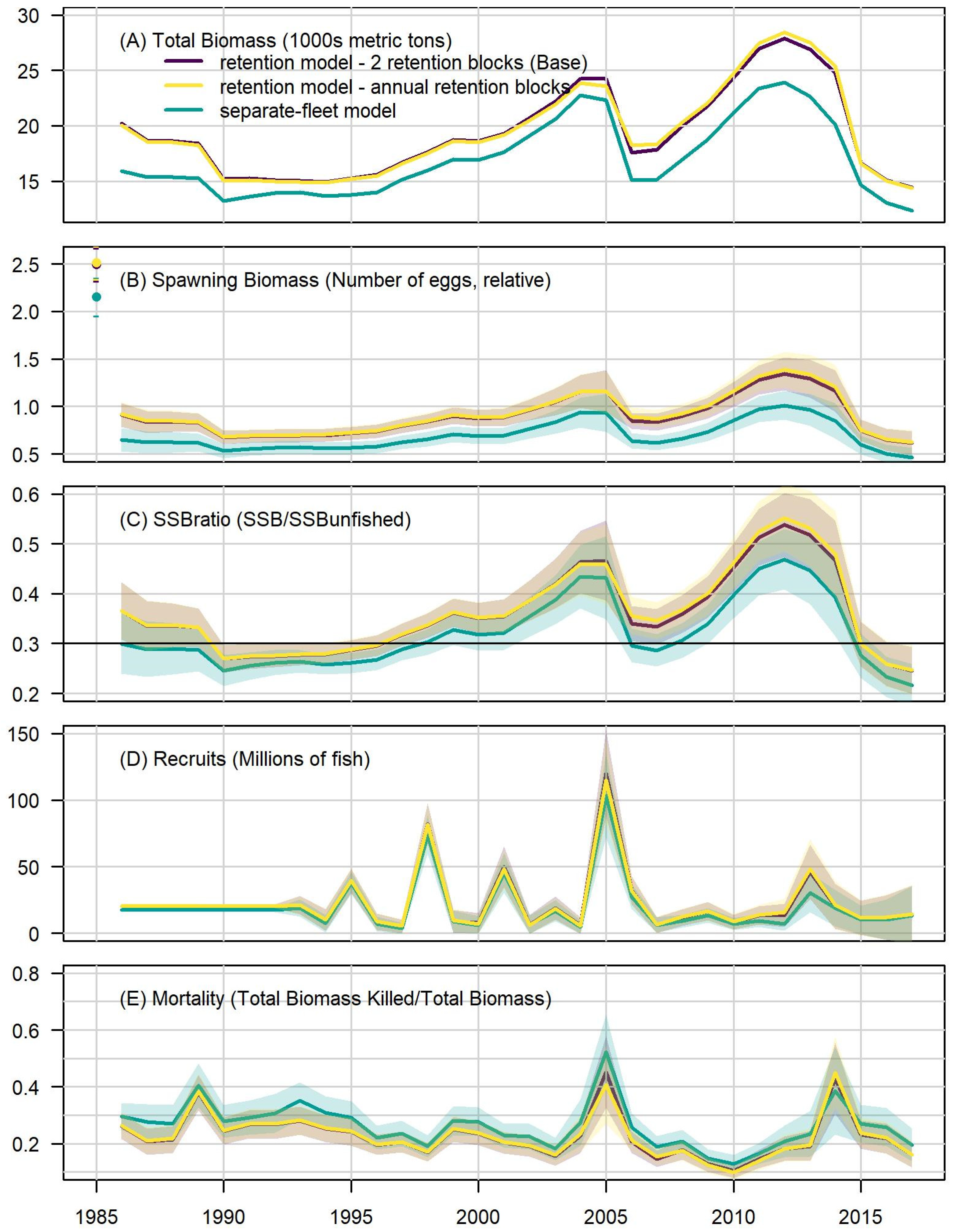
Estimated biomass and spawning stock biomass (SSB) were nearly identical between retention models, whereas the separate-fleet model estimated consistently lower biomass and SSB (Figure 5A,B). Relative trends in the SSB ratio (SSB to unfished SSB) were similar across models, although the separate-fleet model generally estimated a lower SSB ratio, which often fell outside the confidence interval of the estimates obtained from the retention models (Figure 5C). In the terminal year of the assessment, all three model estimates of SSB ratio fell within the uncertainty intervals of the other models.

Estimated recruitments were nearly identical between model runs, with all three models identifying strong cohorts in the same years and peak recruitment in 2005 (Figure 5D). The largest difference occurred in 2013 where the separate-fleet model estimated lower recruitment, although this estimate remained within the confidence interval of the estimates from the retention models. Estimated recruitment variability (${\sigma }_R$) was highest for the separate-fleet model and exhibited more uncertainty than in the base model (Table 2). Estimates of virgin recruitment were very similar between retention models, but lower for the separate-fleet model (Table 2).

Relative trends in estimated fishing mortality rate were generally similar between model runs, although the separate-fleet model estimated higher exploitation rates in almost all years except 2014 (Figure 5E). The separate-fleet model estimated much higher exploitation in 2005 but much lower exploitation in 2014 compared to the retention models, which can be explained by higher estimated red tide mortality in 2005 but lower estimated red tide mortality in 2014 (Table 2). In addition, the separate-fleet model estimated much higher initial fishing mortality estimates for the commercial landings fleets, albeit with greater uncertainty, compared to the retention models (Table 2).

3.2.2. Comparison of Benchmarks

Overall, stock status was similar across models with the Gulf red grouper stock not undergoing overfishing nor deemed overfished in 2017 for any model (

Table 3. Summary of benchmarks and reference points derived from the different modeling approaches for Gulf red grouper. Spawning stock biomass (SSB) is in units of relative number of eggs, whereas F is an exploitation rate (total biomass killed/total biomass).

Criteria	Definition	Retention Model—2 Blocks (Base)	Retention Model—Annual Blocks	Separate-Fleet Model
Mortality Rate Criteria
FMSYproxy = Maximum Fishing Mortality Threshold (MFMT)	Equilibrium fishing mortality that achieves a spawning potential ratio (SPR) of 30%	0.26	0.26	0.29
FCurrent	Average fishing mortality over last three years (2015–2017)	0.20	0.21	0.24
FCurrent/MFMT	Current fishery status	0.78	0.79	0.82
Overfishing in 2017?		No	No	No
Biomass Criteria
SSBMSYproxy	Equilibrium SSB when fishing at FMSYproxy	748,241	754,383	646,482
Minimum Stock Size Threshold (MSST)	0.5×SSBMSYproxy	374,120	377,192	323,241
SSB0	Virgin SSB	2,494,130	2,513,280	2,153,750
SSB2017	SSB in terminal year	613,517	620,817	464,086
SSB2017/MSST	Current stock status	1.64	1.65	1.44
Overfished in 2017?		No	No	No

). However, the separate-fleet model did result in a lower ratio of current SSB (2017) to the Minimum Stock Size Threshold of 1.44 compared to the retention models (1.64–1.65; Table 3), although none of the ratios approached the overfished criterion of 1. The ratios of current F (defined as the average of the last three terminal years, 2015–2017) to the Maximum Fishing Mortality Threshold were similar among models, ranging from 0.78 and 0.82, and were well below the overfishing criterion of 1.

3.2.3. Fleet-Specific Trends in Exploitation Rate

Overall, the annual exploitation rates estimated from discards were considerably and consistently lower than the exploitation rates estimated for landings for each fishing fleet (Figure 6). A few notable exceptions occurred for the recreational fleet where estimates were very similar between 2009 and 2011. Estimated size selectivity patterns for each fleet highlighted the large difference in selectivity between landed fish (solid blue and green lines) and discarded fish (dashed blue and green lines), with discarded fish much smaller (Figure 6 and Figure S10) and younger (Figure S11) than landed fish for each fleet. For the separate-fleet model, time-varying selectivity of red grouper discarded by each fleet shifted to smaller fish over time (Figure 6). While selectivity of red grouper landed by the commercial vertical line fleet was very similar across time periods for the separate-fleet model, more recent landings showed selection for larger red grouper by both the commercial trap fleet (until 2006) and the recreational fleet (Figure 6). Selectivity of red grouper landed by the commercial longline fleet post-IFQ was intermediate between the earliest time period which selected for smaller red grouper and the 1990–2008 time period which selected for the largest red grouper (Figure 6). The estimated selectivity patterns were nearly identical for the retention models and generally fell between the selectivity patterns estimated for landed and discarded fish for the separate-fleet model. For the commercial fleets, estimated annual retention curves since implementation of the IFQ program were very similar and generally reached full retention (i.e., asymptote of 1) whereas annual retention curves were highly variable for the recreational fleet (Figure S12).

3.2.4. Exploitation Patterns

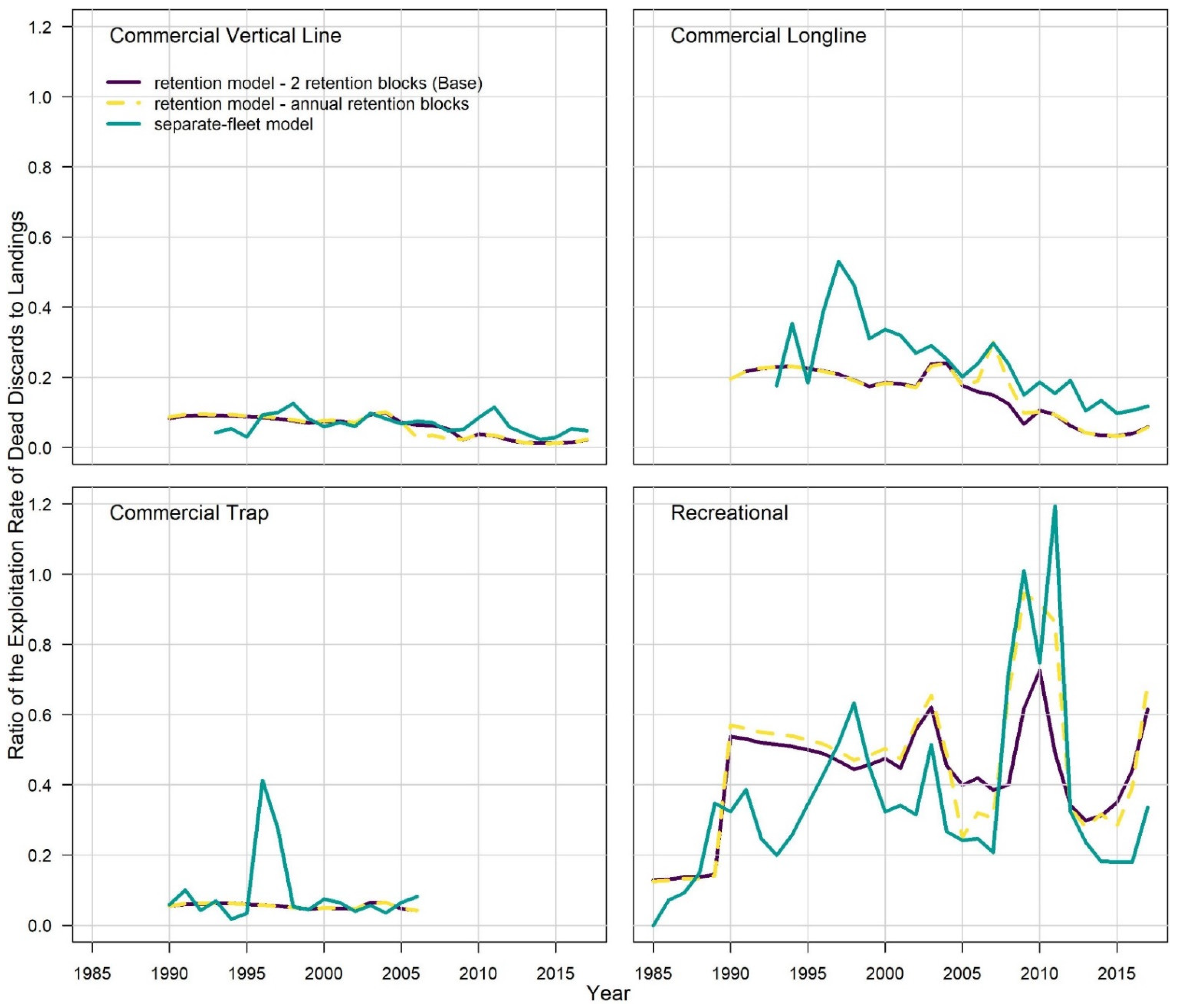
The ratio of exploitation rates associated with dead discards and with landings were more variable over time for the separate-fleet model than for the retention models (Figure 7). Across model runs, dead discards from the commercial trap fleet were generally negligible, with the exception of a peak in 1996 and 1997 for the separate-fleet model, whereas dead discards from the commercial vertical line fleet contributed a relatively small fraction (<15%) of fishing mortality across model runs. In comparison, a higher fraction of fishing mortality was associated with dead discards for the commercial longline fleet and recreational fleet, although trends were quite variable between years for each model but more pronounced for the separate-fleet model. For the recreational fleet, peak ratios near 1.0 indicated that exploitation from discarding was on a similar scale as exploitation from landings. These ratios would have been even higher (i.e., relatively more exploitation due to discarding) had they been computed in numbers rather than biomass, because selectivity of discards favored younger, smaller fish than did selectivity of landings.

4. Discussion

Stock assessments might reasonably ignore discards for fisheries where discarding itself is rare or where release mortality is negligible. Examples of the latter include some invertebrates (e.g., 100% survival of Caribbean Spiny Lobster Panulirus argus released from traps in the U.S. Caribbean [37]) and some species encountered in shallow water where survival is likely (e.g., Lane Snapper Lutjanus synagris [38]). Otherwise, the three most common approaches to handling discards in stock assessments are to lump discard mortalities with landings, to model them with a retention function, or to model them as their own fleet. Lumping discards with landings may be suitable when the selectivity of discards is similar to that of landings, or it may be practical when discard data are too sparse to be informative. Modeling discards explicitly, either with a retention function or as a separate fleet, is preferable when the conditions for ignoring or lumping do not exist. In this paper, we compared the two approaches to modeling discards through simulation analysis and in a case study, with the goals of exploring model behavior and resulting management advice.

Our simulations demonstrated that the separate-fleet model can reproduce or mimic the retention model, if selectivities between the two approaches are configured to be the same. We demonstrated the similarity in results under a range of conditions related to static and time-varying retention. Mathematically, the two approaches should provide identical results whenever Equation (7) (retention-function approach) and Equation (8) (separate-fleet approach) are equal. In practice, however, results from the two approaches can deviate for several reasons. First, discard selectivity derived from a retention function could differ from that of a separate fleet. Second, asymptotic retention is often assumed static, at least within time blocks; the separate-fleet model makes no such assumption, allowing for full flexibility in the annual allocation of fishing effort between landings and discards. Third, release mortality (proportion of released fish that die) is treated differently by the two approaches: the retention-function approach commonly applies it as a multiplier on the fishing mortality rate ($\delta$ in our simulations), and the separate-fleet approach commonly applies it as a multiplier on releases, creating a time series of dead discards for the assessment model to fit by estimating the discard fishing rate.

Indeed, treatment of release mortality can be a source of error in both approaches. Release mortality is typically estimated from field data as a proportion in units of deaths per released fish [2,3]. Applying this proportion as a multiplier on the instantaneous fishing rate (units of per time), as in the retention-function approach, is not technically correct; however, this practice does appear to be a reasonable approximation, especially when fishing rates are low (~<0.2). In contrast, application of the separate-fleet model would entail fitting predicted dead discards to observed dead discards, where observed values would first be estimated by multiplying the release mortality proportion by the total number of released fish. This practice is the more technically correct application of a release mortality proportion, yet it does tacitly assume that each individual fish is caught only once or that release mortality does not vary with recapture, which may not be true [39].

Explicitly modeling discards in stock assessments can be challenged by quantity and quality of relevant data, combined with an incomplete understanding of fisher behavior. The Gulf red grouper case study underscored the importance of having length composition of discarded fish, which allowed for an investigation of whether selectivity differed between landed and discarded fish. Since 2007, the NMFS Observer Program has collected length composition data of fish both landed and discarded by the commercial sector throughout the Gulf of Mexico [40]. Since sampling began prior to the implementation of the Individual Fishing Quota (IFQ) program, trends in discards can be compared both before and after its implementation. The FWRI At-Sea Observer Program has collected length composition data of discarded and landed fish for recreational headboats (since 2005) and charterboats (since 2009) throughout the eastern Gulf of Mexico [41]. Each of these data sources are critical for understanding how discarding behavior has changed through time within the commercial and recreational sectors. While the majority of discarded red grouper are below the size limit [36], some discarding of legal fish does occur, likely due to management regulations such as recreational bag limits or lack of IFQ in the commercial fishery [35,36]. In addition, length composition data on discarded fish enables the assessment model to estimate retention functions or selectivity of a discards fleet. In the absence of such information, assumptions must be made regarding the shape of the retention function or the selectivity curve.

While the overall outcome of the red grouper stock assessment did not change across configurations, some noteworthy differences were identified. The separate-fleet model for red grouper revealed highly variable differences in dead discards to landings ratios for the commercial longline and recreational fisheries. For both the commercial vertical line and longline fisheries, some of the highest dead discards to landings ratios occur in years after the implementation of the IFQ. For the recreational fleet, estimated dead discards were nearly as high as landings in 2011. Although the recreational bag limit for red grouper increased from two fish to four fish per person per day in 2011, this regulation likely would have reduced discards. A comprehensive assessment of state and federal management regulations across the various species in this mixed-species reef fish fishery is paramount in helping to understand the indirect effects of management regulations on reef fish species. For example, the 2007 implementation of an IFQ for Gulf red snapper Lutjanus campechanus caused a shift in targeting and fishing effort toward red grouper, among other groupers and snappers [42].

The red grouper models differed in their estimates of exploitation rates, with the separate-fleet model estimating higher initial fishing mortality for almost all of the landings fleets and overall larger exploitation rates. For the retention model, the selectivity curve of exploited fish peaked between the selectivity curves of discards and landings from the separate-fleet model. Starting values for initial equilibrium catches for the landings fleets were identical across model runs and were approximated from the average landings of red grouper in the first five years of the time series. No initial catches were input for the discard fleets. The separation of landings F and discards F in the separate-fleet model resulted in higher and more variable estimated initial fishing mortality rates for all fleets compared to the retention models, which likely led to lower estimates of initial SSB and recruitment.

The red grouper case study, considered data rich given fleet-specific discard data, highlights a few additional challenges beyond data availability when modeling discards. First, Gulf red grouper discards for each fleet were assigned a single uncertainty estimate in the absence of annual uncertainty estimates. Similar error estimates (~0.3) have been used for other Gulf stocks including red snapper [43] and gray snapper Lutjanus griseus [44]. Better characterization of discard uncertainty can greatly assist modeling efforts, as demonstrated during the Gulf gag grouper Mycteroperca microlepis assessment [45] for which annual uncertainty estimates were available for all fleets except recreational headboats. Second, one must choose an appropriate error distribution for modeling discards. The Gulf red grouper assessment assumed a lognormal error distribution, which may not be an appropriate characterization in all cases. Currently, error distributions in Stock Synthesis are restricted to lognormal for landings, and therefore dead discards “landed” by discards as fleets. In contrast, error distributions for discards can follow a Student’s t-distribution, a normal distribution, or a lognormal distribution [30]. Other distributions, such as negative binomial, could prove useful for modeling discards [27]. Third, “data availability” may often be better described as a continuum than as a binary condition. Many stocks are not data poor or data rich, but rather “data moderate,” forcing analysts to decide whether the data are sufficient for modeling purposes and whether knowledge gaps can be filled with reasonable assumptions. For example, sparse discard data, i.e., where annual sample sizes are low, can be included in Stock Synthesis using “super-periods,” in which annual discards are represented by the mean or median within time blocks (e.g., [46]).

Which approach—retention-function or separate-fleet—is best for modeling discards? Although our study was not designed to address this question, the answer is likely case-specific and will depend on the amount and source of year-to-year variability in discarding behavior. In a fishery that is clean (i.e., little bycatch) and if discarding behavior is relatively stable through time, the static retention-function approach is likely best because it describes the system with the fewest parameters. Similarly, if the annual variability in observed discards is due primarily to observation error, the static retention-function approach might be more suitable, as discard estimates would be less affected by noise in the data. However, in addition to observation error, the discarding process itself is generally dynamic, affected by a multitude of factors [15,16,47,48]. For example, a temporal shift toward landings per unit of fishing effort (and away from discards) might occur if the stock becomes more desirable with an increase in market value. A shift toward discards (per unit of fishing effort) might occur when harvest restrictions are tightened yet effort does not decline, as might occur in a mixed-stock fishery. For fisheries where discarding behavior remains unstudied, what we have learned from the existing studies may provide a good platform from which to extrapolate. In other words, unless contrary evidence exists, the assumption of year-to-year variability in discarding behavior would seem plausible. Such variability is naturally accounted for by the separate-fleet approach, given the separation of fishing rates toward landings and dead discards, such that no assumption is made about the annual allocation of fishing effort. The hypothesis that discards are proportional to catch or effort was examined by Rochet and Trenkel [15], who found that it lacks empirical support. The retention-function approach is not typically configured for variability in discarding behavior beyond the application of time blocks. However, this is not a constraint of the approach itself; time-varying retention functions can be estimated [21,26,49], perhaps annually in cases where the supporting data exist. A comprehensive simulation study utilizing operating models and estimation models would be beneficial for answering the question of which approach works best under various levels of observation and process error.

When the relative importance of fishing rates toward landings and discard components varies over time, as with the fleet-specific model or with time-varying retention functions, computation of reference points requires weighting those components in some way. One common approach is to use the geometric mean fishing rate computed from the terminal N years of the assessment (e.g., last three years). In contrast, the time-invariant retention approach does not require such weighting, as the allocation of fishing effort into landings and discards is fixed. Thus, the difference between modeling approaches can have management implications. In a management system based on output controls, such as in U.S. fishery management, the choice of modeling approach affects MSY and F_MSY, and consequently, the Annual Catch Limits that would be produced by a stock assessment model. In the Gulf red grouper case study, projections taking the approach of discards as a separate fleet assumed that the level of dead discards in each projection year was similar to the terminal year of the assessment.

5. Conclusions

A general consensus exists regarding the importance of including discards in stock assessment models [25,26,27]. Lumping estimates of discard mortalities with landings is a practical approach if the level of discarding is small relative to landings, if selectivity of discards is the same as that of landings, or if discard data are too sparse to be informative. When modeling discards explicitly, the two most common approaches are to treat discards as their own fleet or to model them with a retention function. Here, we demonstrated mathematically and through simulation that the two approaches are identical, if selectivity functions are configured the same. In practice, however, the approaches to modeling discards can result in different assessment outcomes, as demonstrated through our case study of Gulf red grouper. Which approach makes best use of discard data is likely circumstantial, depending on the relative contributions of observation and process errors in discarding, and further research is needed to provide general guidance on model selection.

References

1. Davies, R.W.D.; Cripps, S.J.; Nickson, A.; Porter, G. Defining and estimating global marine fisheries bycatch. Mar. Policy 2009, 33, 661–672. [Google Scholar] [CrossRef]
2. Davis, M.W. Key principles for understanding fish bycatch discard mortality. Can. J. Fish. Aquat. Sci. 2002, 59, 1834–1843. [Google Scholar] [CrossRef]
3. Bartholomew, A.; Bohnsack, J.A. A review of catch-and-release angling mortality with implications for no-take reserves. Rev. Fish Biol. Fish. 2005, 15, 129–154. [Google Scholar] [CrossRef]
4. Gillespie, A. Wasting the oceans: Searching for principles to control bycatch in international law. Int. J. Mar. Coast. Law 2002, 17, 161–193. [Google Scholar] [CrossRef]
5. Harrington, J.M.; Myers, R.A.; Rosenberg, A.A. Wasted fishery resources: Discarded by-catch in the USA. Fish Fish. 2005, 6, 350–361. [Google Scholar] [CrossRef]
6. Zeller, D.; Cashion, T.; Palomares, M.; Pauly, D. Global marine fisheries discards: A synthesis of reconstructed data. Fish Fish. 2018, 19, 30–39. [Google Scholar] [CrossRef] [Green Version]
7. Crowder, L.B.; Murawski, S.A. Fisheries bycatch: Implications for management. Fisheries 1998, 23, 8–17. [Google Scholar] [CrossRef]
8. Zhou, S. Fishery by-catch and discards: A positive perspective from ecosystem-based fishery management. Fish Fish. 2008, 9, 308–315. [Google Scholar] [CrossRef]
9. Heath, M.R.; Cook, R.M.; Cameron, A.I.; Morris, D.J.; Speirs, D.C. Cascading ecological effects of eliminating fishery discards. Nat. Commun. 2014, 5, 3893. [Google Scholar] [CrossRef] [Green Version]
10. Kelleher, K. Discards in the World’s Marine Fisheries. An Update; FAO Fisheries Technical Paper 470; Food and Agriculture Organization: Rome, Italy, 2005; 131p. [Google Scholar]
11. Catchpole, T.L.; Frid, C.L.J.; Gray, T.S. Discards in North Sea fisheries: Causes, consequences and solutions. Mar. Policy 2005, 29, 421–430. [Google Scholar] [CrossRef]
12. Campana, S.E. Transboundary movements, unmonitored fishing mortality, and ineffective international fisheries management pose risks for pelagic sharks in the Northwest Atlantic. Can. J. Fish. Aquat. Sci. 2016, 73, 1599–1607. [Google Scholar] [CrossRef]
13. Borges, L. The evolution of a discard policy in Europe. Fish Fish. 2015, 16, 534–540. [Google Scholar] [CrossRef]
14. Catchpole, T.L.; Elliott, S.; Peach, D.; Mangi, S.C.; Gray, T.S. How to deal with the EU landings obligation: Lessons from an English discard ban sea trial. ICES J. Mar. Sci. 2018, 75, 270–278. [Google Scholar] [CrossRef]
15. Rochet, M.J.; Trenkel, V.M. Factors for the variability of discards: Assumptions and field evidence. Can. J. Fish. Aquat. Sci. 2005, 62, 224–235. [Google Scholar] [CrossRef]
16. Feekings, J.; Bartolino, V.; Madsen, N.; Catchpole, T. Fishery discards: Factors affecting their variability within a demersal trawl fishery. PLoS ONE 2012, 7, e36409. [Google Scholar] [CrossRef] [Green Version]
17. Pascoe, S. Bycatch Management and the Economics of Discarding; FAO Fisheries Technical Paper No. 370; Food and Agriculture Organization: Rome, Italy, 1997; 137p. [Google Scholar]
18. Depestele, J.; Vandemaele, S.; Vanhee, W.; Polet, H.; Torreele, E.; Leirs, H.; Vincx, M. Quantifying causes of discard variability: An indispensable assistance to discard estimation and a paramount need for policy measures. ICES J. Mar. Sci. 2011, 68, 1719–1725. [Google Scholar] [CrossRef]
19. Batsleer, J.; Hamon, K.G.; van Overzee, H.M.J.; Rijnsdorp, A.D.; Poos, J.J. High-grading and over-quota discarding in mixed fisheries. Rev. Fish. Biol. Fish. 2015, 25, 715–736. [Google Scholar] [CrossRef] [Green Version]
20. Cass-Calay, S.L.; Arnold, W.S.; Bryan, M.D.; Schull, J. Report of the US Caribbean Fishery-Independent Survey Workshop. NOAA Technical Memorandum NMFS-SEFSC-688, 2016. Available online: https://repository.library.noaa.gov/view/noaa/10477 (accessed on 4 October 2021).
21. Stratoudakis, Y.; Fryer, R.J.; Cook, R.M. Discarding practices for commercial gadoids in the North Sea. Can. J. Fish. Aquat. Sci. 1998, 55, 1632–1644. [Google Scholar] [CrossRef]
22. Garner, S.B.; Patterson, W.F. Direct observation of fishing effort, catch, and discard rates of charter boats targeting reef fishes in the northern Gulf of Mexico. Fish. Bull. 2015, 113, 157–166. [Google Scholar] [CrossRef] [Green Version]
23. Heath, M.R.; Cook, R.M. Hind-casting the quantity and composition of discards by mixed demersal fisheries in the North Sea. PLoS ONE 2015, 10, e0117078. [Google Scholar] [CrossRef] [Green Version]
24. Williams, E.H. The effects of unaccounted discards and misspecified natural mortality on harvest policies based on estimates of spawners per recruit. N. Am. J. Fish. Manag. 2002, 22, 311–325. [Google Scholar] [CrossRef]
25. Punt, A.E.; Smith, D.C.; Tuck, G.N.; Methot, R.D. Including discard data in fisheries stock assessments: Two case studies from south-eastern Australia. Fish. Res. 2006, 79, 239–250. [Google Scholar] [CrossRef]
26. Aarts, G.; Poos, J.J. Comprehensive discard reconstruction and abundance estimation using flexible selectivity functions. ICES J. Mar. Sci. 2009, 66, 763–771. [Google Scholar] [CrossRef] [Green Version]
27. Cook, R.M. Inclusion of discards in stock assessment models. Fish Fish. 2019, 20, 1232–1245. [Google Scholar] [CrossRef]
28. Methot, R.D., Jr.; Wetzel, C.R. Stock synthesis: A biological and statistical framework for fish stock assessment and fishery management. Fish. Res. 2013, 142, 86–99. [Google Scholar] [CrossRef]
29. R Core Team. R: A Language and Environment for Statistical Computing; R Foundation for Statistical Computing: Vienna, Austria, 2021; Available online: https://www.R-project.org/ (accessed on 4 October 2021).
30. Methot, R.D., Jr.; Wetzel, C.R.; Taylor, I.G. Stock Synthesis User Manual Version 3.30.12; NOAA Fisheries: Seattle, WA, USA, 2018; 235p.
31. Sagarese, S.R.; Vaughan, N.R.; Walter, J.F., III; Karnauskas, M. Enhancing single-species stock assessments with diverse ecosystem perspectives: A case study for Gulf of Mexico Red Grouper (Epinephelus morio) and red tides. Can. J. Fish. Aquat. Sci. 2021, 78, 1168–1180. [Google Scholar] [CrossRef]
32. Pulver, J.R.; Lombardi, L.; Scott-Denton, E. Summary of Commercial Red Grouper (Epinephelus morio) Catch Data Based on Fishery Observer Coverage of the Gulf of Mexico Reef Fish Fishery; SEDAR42-DW-01; SEDAR: North Charleston, SC, USA, 2014; 40p. [Google Scholar]
33. Gray, A.; Sauls, B. Size Distribution of Red Grouper Observed in for-Hire Recreational Fisheries in the Gulf of Mexico; SEDAR42-DW-14; SEDAR: North Charleston, SC, USA, 2014; 22p. [Google Scholar]
34. Lazarre, D. A Summary of Red Grouper Size Distribution Data from Recreational Fishery Surveys in the Gulf of Mexico; SEDAR61-WP-13; SEDAR: North Charleston, SC, USA, 2018; 17p. [Google Scholar]
35. SEDAR61—Gulf of Mexico Red Grouper Stock Assessment Report; SEDAR: North Charleston, SC, USA, 2019; 285p, Available online: http://sedarweb.org/sedar-61 (accessed on 4 October 2021).
36. Pulver, J.R.; Stephen, J.A. Factors that influence discarding in the Gulf of Mexico commercial grouper-tilefish IFQ reef fish fishery. Fish. Res. 2019, 218, 218–228. [Google Scholar] [CrossRef]
37. SEDAR 57—U.S. Caribbean Spiny Lobster Stock Assessment Report; SEDAR: North Charleston, SC, USA, 2019; 232p, Available online: http://sedarweb.org/sedar-57 (accessed on 4 October 2021).
38. SEDAR 49—Gulf of Mexico Data-Limited Species Stock Assessment Report; SEDAR: North Charleston, SC, USA, 2016; 618p, Available online: http://sedarweb.org/sedar-49 (accessed on 4 October 2021).
39. Runde, B.J.; Buckel, J.A.; Shertzer, K.W.; Bacheler, N.M.; Rudershausen, P.J.; Sauls, B. Repetitive capture of marine fishes: Implications for estimating number and mortality of releases. ICES J. Mar. Sci. 2020, 77, 2905–2917. [Google Scholar] [CrossRef]
40. Scott-Denton, E.; Cryer, P.F.; Gocke, J.P.; Harrelson, M.R.; Kinsella, D.L.; Pulver, J.R.; Smith, R.C.; Williams, J.A. Descriptions of the US Gulf of Mexico reef fish bottom longline and vertical line fisheries based on observer data. Mar. Fish. Rev. 2011, 73, 1–26. [Google Scholar]
41. Sauls, B.; Ayala, O. Circle hook requirements in the Gulf of Mexico: Application in recreational fisheries and effectiveness for conservation of reef fishes. Bull. Mar. Sci. 2012, 88, 667–679. [Google Scholar] [CrossRef]
42. Agar, J.J.; Stephen, J.A.; Strelcheck, A.; Diagne, A. The Gulf of Mexico red snapper IFQ program: The first five years. Mar. Resour. Econ. 2014, 29, 177–198. [Google Scholar] [CrossRef]
43. SEDAR 52—Gulf of Mexico Red Snapper Stock Assessment Report; SEDAR: North Charleston, SC, USA, 2018; 434p, Available online: http://sedarweb.org/sedar-52 (accessed on 4 October 2021).
44. SEDAR 51—Gulf of Mexico Gray Snapper Stock Assessment Report; SEDAR: North Charleston, SC, USA, 2018; 428p, Available online: http://sedarweb.org/sedar-51 (accessed on 4 October 2021).
45. SEDAR 72—Gulf of Mexico Gag Grouper Stock Assessment Report; SEDAR: North Charleston, SC, USA, 2021; 318p, Available online: http://sedarweb.org/sedar-72 (accessed on 4 October 2021).
46. SEDAR 28 Update—Gulf of Mexico Cobia Stock Assessment Report; SEDAR: North Charleston, SC, USA, 2021; 147p, Available online: http://sedarweb.org/sedar-28 (accessed on 4 October 2021).
47. Catchpole, T.L.; Enever, R.; Maxwell, D.L.; Armstrong, M.J.; Reese, A.; Revill, A.S. Constructing indices to detect temporal trends in discarding. Fish. Res. 2011, 107, 94–99. [Google Scholar] [CrossRef]
48. Tsagarakis, K.; Palialexis, A.; Vassilopoulou, V. Mediterranean fishery discards: A review of the existing knowledge. ICES J. Mar. Sci. 2014, 71, 1219–1234. [Google Scholar] [CrossRef] [Green Version]
49. Borges, L.; Zuur, A.F.; Rogan, E.; Officer, R. Modelling discard ogives from irish demersal fisheries. ICES J. Mar. Sci. 2006, 63, 1086–1095. [Google Scholar] [CrossRef] [Green Version]
Figure 1. Selectivity curves used in simulations, based on parameter values shown in Table 1 for Simulation 1. (A) Selectivity of the catch (yellow, solid) and the retention function (purple, dashed). (B) Resulting selectivity of landings (yellow, solid) and of discards (purple, dashed).
Fishes 07 00007 g001
Figure 2. Time series of data inputs incorporated into the Gulf red grouper stock assessment model and relevant management regulations (with values specified where necessary).
Fishes 07 00007 g002
Figure 3. Results of Simulation 1 using the retention model (blue, solid) or separate-fleet model (green, dashed). (A) Fishing rate (y−1) toward discard mortality. (B) Fishing rate (y−1) toward landings. (C) Recruitment. (D) Abundance. (E) Dead discards. (F) Landings. Note that blue and green curves overlap in each panel.
Fishes 07 00007 g003
Figure 4. Exploitation rates associated with landings and dead discards, as indicated on panels, in simulations using the retention model (blue, solid) or separate-fleet model (green, dashed). (A) Simulation 1. (B) Simulation 2. (C) Simulation 3. (D) Simulation 4. Note that blue and green curves overlap in each panel.
Fishes 07 00007 g004
Figure 5. Derived quantities from the Gulf red grouper models where retention was modeled using two time blocks (base model; purple), annual time blocks (yellow), or where discards were modeled as a separate-fleet (teal). (A) Total biomass. (B) Unfished (top left, dots with dashed lines indicative of 95% confidence intervals) and annual spawning stock biomass (SSB). (C) SSB ratio, defined as the ratio of SSB to unfished SSB (horizontal line identifies target value of 0.3). (D) Recruitment. (E) Mortality in terms of exploitation, defined as the proportion of total biomass killed to total biomass (with red tide mortality included in 2005 and 2014). The 95% confidence intervals surrounding each curve are indicated by the relevant color.
Fishes 07 00007 g005
Figure 6. Comparison of estimated exploitation rates (total biomass killed/total biomass) and estimated length-based selectivity patterns by fishery for each Gulf red grouper model implementing different approaches to including discards. Selectivity time blocks are for landings (L) or discards (D).
Fishes 07 00007 g006
Figure 7. Comparison of exploitation rates from dead discards (total biomass discarded dead/total biomass) to exploitation rates from landings (total biomass landed/total biomass) for each fishery as estimated for each Gulf red grouper model implementing different approaches to including discards.
Fishes 07 00007 g007