The Relationship Between Respiration Rates and Electron Transport System Activity in Fish

Abstract

Fishes contribute to the biological carbon pump, yet their overall role remains poorly constrained due to the difficulty of obtaining direct metabolic measurements and, consequently, is poorly understood. Electron transport system (ETS) activity is commonly used as a proxy for potential respiration, but its application requires an appropriate relationship between respiration (R, measured as oxygen consumption MO₂) and ETS activity. Here, we examined the relationship between swimming activity, oxygen consumption, and ETS activity in juvenile Sparus aurata using swimming-tunnel respirometry. Oxygen consumption increased with swimming speed following a four-parameter sigmoidal model, whereas ETS activity remained independent of short-term changes in activity. Normalizing respiration by ETS produced R/ETS ratios ranging from 0.17 to 0.71, values consistent with those reported for zooplankton and micronekton. Lower ratios correspond to minimal aerobic demand and may represent quiescent behaviour, while higher ratios reflect elevated demands associated with active movement or feeding. These ratios are suggested for the assessment of respiration rates from ETS activity during diel vertical migration in the ocean to improve estimates of respiratory flux. However, methodological issues related to ETS activity in different body regions must be solved to enable reliable measurements.

1. Introduction

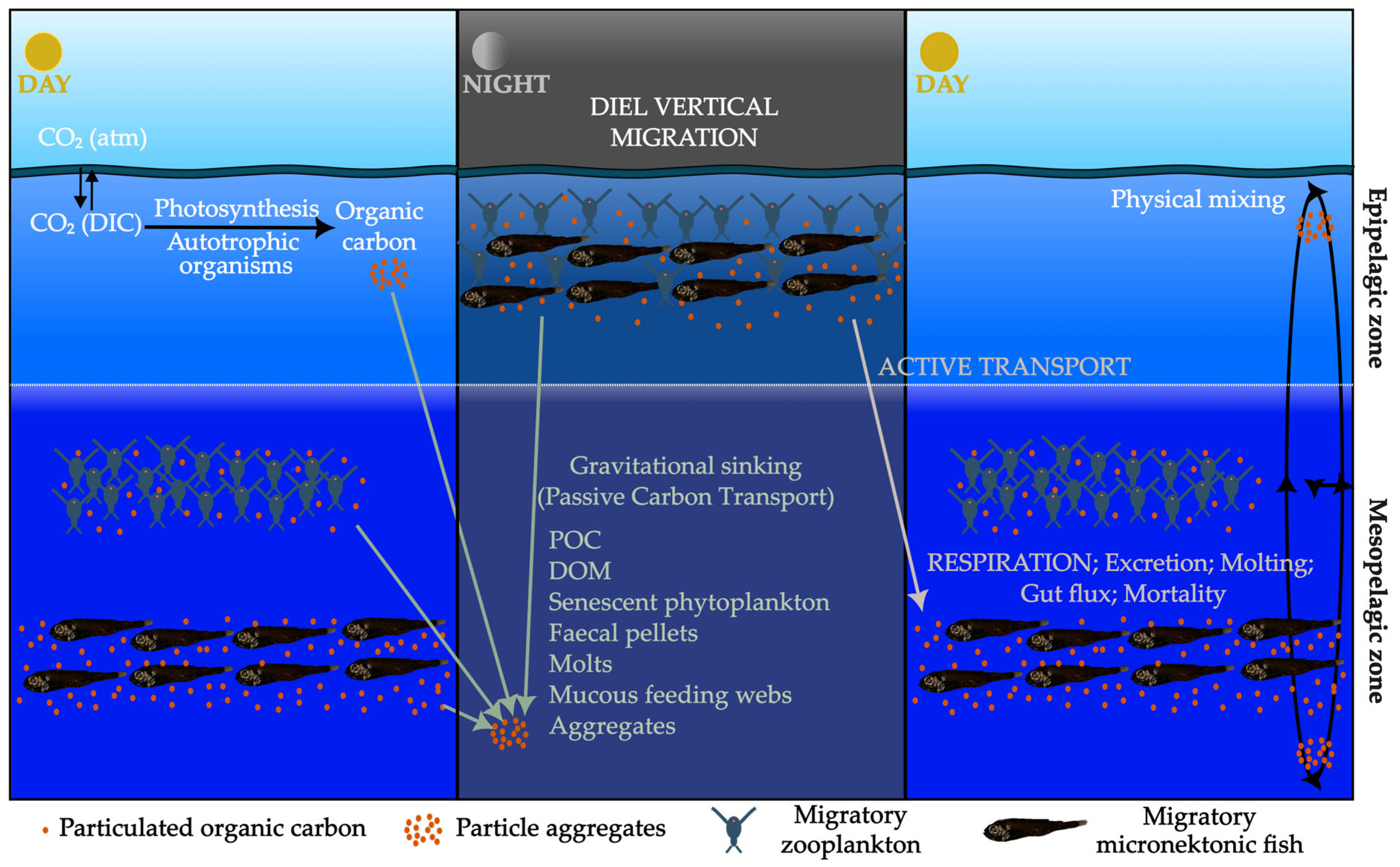
The ocean plays a central role in the global carbon cycle, acting as a major sink for anthropogenic carbon through its export from the surface layer and subsequent, sequestration, which leads to long-term storage in the deep sea. Carbon is mainly found as dissolved inorganic carbon (DIC) resulting from the air–sea gas exchange of atmospheric CO₂ with the ocean surface. It is transported downward by the movement of water masses (physical pump) or assimilated by autotrophic organisms through photosynthesis, entering the trophic web [1,2,3]. Carbon is transported into the interior ocean through three main mechanisms: the solubility pump, the biological pump, and the marine carbonate pump [1,4]. Other studies [5,6,7] also proposed a fourth mechanism, the microbial carbon pump. The biological pump refers to the process by which carbon is transferred from the ocean’s surface layers to the deep ocean via primary production by marine phytoplankton, which converts DIC and nutrients into organic matter through photosynthesis [8]. Part of this carbon is transported through the water column to the deep sea as result of a chain of biologically mediated processes [2,9]. Particulate and dissolved matter flux (including senescent phytoplankton, fecal pellets, moults, mucous feeding webs, and aggregates of these materials) is transported to deeper layers by gravity (passive sinking), physical mixing, and active transport resulting from the diel vertical migration (DVM) of zooplankton and micronekton [10,11] (Figure 1).

DVM is a daily movement of organisms through the water column observed across all oceans [12]. This migrating biomass is mainly composed of zooplankton (mainly large copepods and euphausiids) and micronekton (mainly mesopelagic fish, decapods, and cephalopods) [13,14]. These migrations play an important role in the biological pump [15,16,17] as animals feed in the epipelagic layer at night and metabolize the ingested food in deeper waters during the day. Thus, this fauna actively contributes to carbon transport by respiring and excreting carbon at depth, moulting there, and/or being preyed on by deeper-dwelling fauna. By egesting fecal pellets, they also contribute to the passive flux [3,15,18]. Micronekton exhibit higher mobility and deeper migration ranges than zooplankton and, therefore have a higher capacity to export carbon to deeper waters [19]. While zooplankton digest the gut contents in minutes [20], micronekton require hours or days for digestion [21,22], and their fecal pellets sink rapidly [23] increasing the rate of the vertical flux of particulate organic matter. Thus, micronekton appear to be more efficient than zooplankton in transporting carbon to deeper layers.

Until the 1990s, passive flux was considered the dominant process in the vertical carbon transport. However, after the pioneering paper by Longhurst et al. [24] the importance of active carbon flux mediated by vertical migrants was recognized [16,25,26,27,28]. Among the physiological processes that occur at depth, respiration is one of the most important transport pathways of migrant fauna. It is defined as the oxidation of organic compounds within cells, which produce CO₂ as a by-product (or remineralize carbon), and is directly linked to metabolic activity and, consequently, to the activity of individuals. Therefore, measuring respiration rates, that is, how much oxygen is consumed to produce energy, is essential to better understand active flux. Traditionally, oceanographers focused on zooplankton due to their larger population biomass compared to micronekton [29]. As a result, most studies on active flux were biassed by a lack of information about micronekton active flux. This knowledge gap is also related to the difficulty of sampling micronekton due to their irregular distribution, larger body size, and motility [28].

Among micronekton, fishes are a key component of the mesopelagic fauna performing DVM and thus play a prominent role in active flux [30,31]. However, the in vivo respiration rates of mesopelagic and bathypelagic fish remain a major gap in our understanding of the biological carbon pump. Maintaining these organisms alive after sampling for metabolic experiments remains a challenge. A practical approach to estimate aerobic metabolic rates in deep sea species is the measurement of the enzyme activity of the electron transport system (ETS; [32]). Because the assay is performed in vitro under saturating (non-limiting) substrate and cofactor concentrations, ETS activity serves as a proxy for the maximal mitochondrial oxygen-processing capacity for energy production. This enzymatic assay was originally developed for phytoplankton and later modified and adapted to zooplankton samples [33]. Since ETS activity remains stable during sampling [32], it can be considered a suitable proxy for respiration (R) in deep-sea organisms. However, calibration between the ETS activity and actual respiration rates is necessary to obtain reliable estimations. Previous calibrations in fish were afforded by Ikeda [34] using gobies and pomacentrids to obtain R/ETS values. However, these experiments were performed in sealed glass bottles without controlling for hypoxia, and swimming activity was not considered. Given that mesopelagic fishes perform diel vertical migrations for extended periods (approximately 4 h), it is of interest to understand how oxygen consumption varies with activity level and how ETS activity could be used as a proxy. This comparison allows for the calculation of R/ETS ratios under different swimming conditions during the diel migration.

In this study, we aim to establish a quantitative relationship between ETS activity and oxygen consumption in actively swimming fish, as a foundational step toward developing a reliable method for estimating respiration rates in mesopelagic species. To avoid the need for whole-body homogenization, we also evaluated ETS activity across different body regions to identify the localized sampling zones that best represent total enzymatic activity. We used Sparus aurata as a practical model fish due to its availability and suitability for controlled respirometry. The insights gained from this experimental approach provide a first approximation of R/ETS values under defined activity levels, offering a methodological framework for future assessments of active carbon flux mediated by vertically migrating micronekton.

2. Materials and Methods

2.1. Animals

A total of 21 juvenile gilthead sea breams (Sparus aurata) from the same farm-raised cohort of unknown sex (immature gonads) were used in the experiments. Mean wet mass (WM) was 47.11 ± 9.81 g, length (L) 12.09 ± 0.80 cm, height (H) 4.43 ± 0.47 cm, and width (W) 1.78 ± 0.32 cm (mean ± standard deviation). Detailed individual morphometrics are shown in Table S1. Fish were fasted for 24 h prior to experimentation and transported within the same facility from one experimental unit to another in a closed bucket containing seawater taken from their holding tanks. Transport duration was minimal (a few minutes), ensuring stable environmental conditions and minimizing handling stress. All fish were anesthetised with MS-222 (Sigma-Aldrich, St. Louis, MO, USA, E10521) and euthanised by immersion in liquid nitrogen (−196 °C) at the end of the experiment to collect muscle samples for ETS activity measurements.

2.2. Respirometry

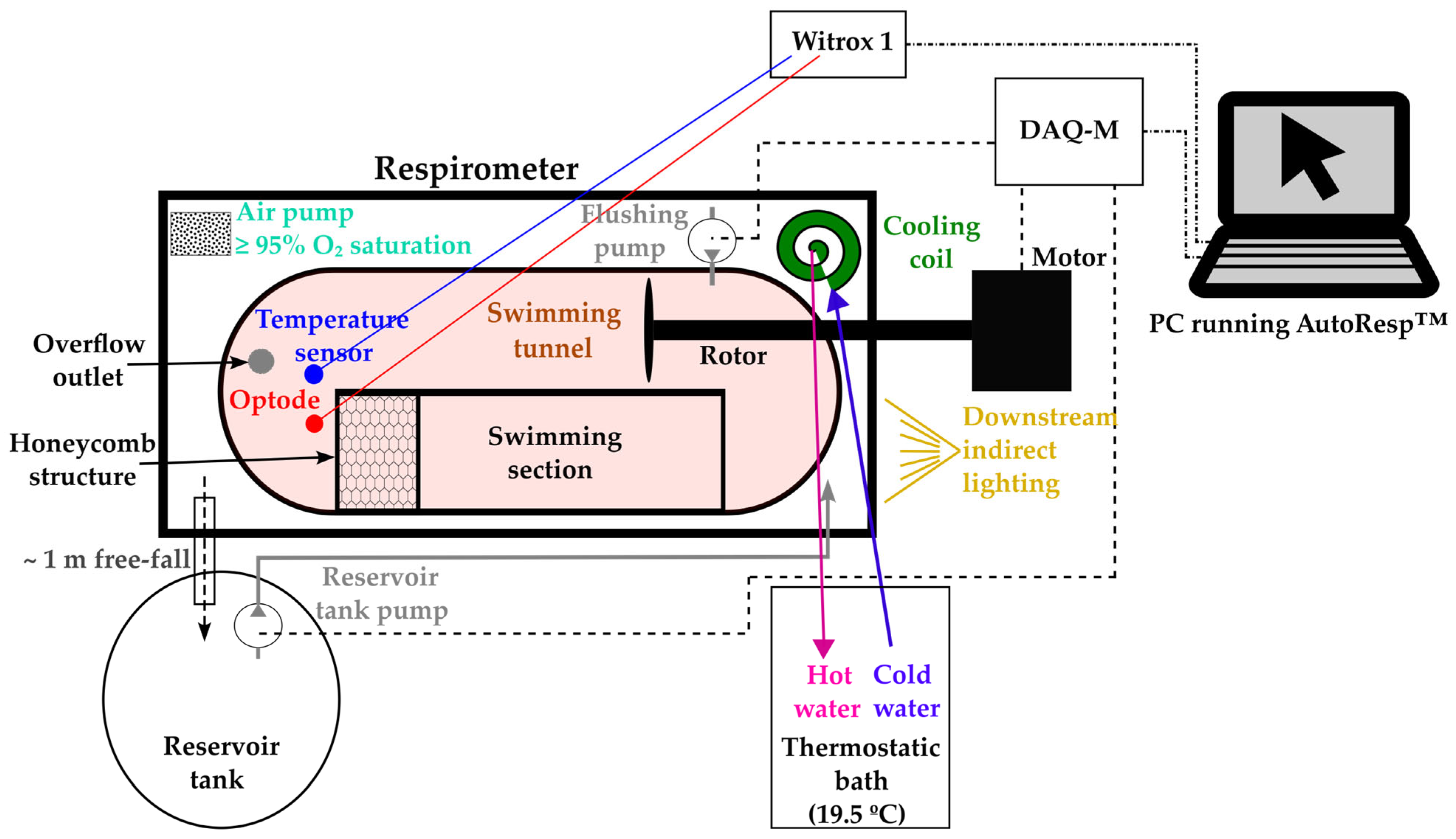
An intermittent flow respirometre (5 litres, Loligo^® System, Viborg, Denmark, Figure 2) was used to measure oxygen consumption (MO₂, mg O₂·kg WM⁻¹·h⁻¹) as a function of swimming speed (in body lengths per second, BL·s⁻¹). The swimming tunnel was submerged in a respirometer tank, which served as a temperature-controlled, high-oxygen water reservoir. From here, water was flushed by a pump to the inner of the swimming tunnel during flushing times. Water flowed freely from the respirometer to a reservoir tank, where it was recirculated back by a second pump. Temperature was maintained at 19.5 °C using a thermostatic bath connected to a cooling coil inserted into the respirometer. Temperature inside the swimming tunnel was monitored using a sensor HTF50 Pt1000 Class (S+S Regeltechnik GmbH, Nuremberg, Germany). Water oxygen saturation in the swimming tunnel was measured using dipping probe oxygen mini sensor (optodes, PreSens Precision Sensing GmbH, Regensburg, Germany). Both sensors, oxygen and temperature, were connected to a Witrox 1 single channel oxygen meter (Loligo^® Systems, Viborg, Denmark). Oxygen saturation levels were kept above 95% in the respirometer water by an air pump and by the water that had free-fallen to the recover water tank (1 m approx.).

Flushing and reservoir tank pumps, as well as the current speed, were controlled via a DAQ-M instrument (Loligo^® Systems, Viborg, Denmark) connected to a computer running AutoResp^TM 2.2.0 software [35] (Loligo^® Systems, Viborg, Denmark). The swimming section of the swimming tunnel was 30 × 7.5 × 7.5 cm (L × W × H). The internal recirculation flow passed through an upstream honeycomb structure to generate microturbulence and ensure homogeneous oxygen distribution. Water speed was calibrated using a vane wheel flow sensor (Höntzsch GMbH, Waiblingen, Germany) and a linear correlation was established between water velocity and motor controller output voltage.

2.3. Experimental Protocol

As stated above, fish were fasted for 24 h prior to respirometry in order to reduce excretion and egestion residues into the recirculation system and to ensure no oxygen consumption due to digestion processes [36,37]. Fish mass, length, depth, and width were measured before placing the fish in the swimming tunnel, allowing for correction for solid blocking effects using AutoResp^TM software [38,39]. Acclimation lasted 5 h, the minimum time suggested by the manufacturer in the device manual. The swimming speed during the acclimation time was 0.5 BL·s⁻¹. During acclimation and measurements, the system was kept in dim light by covering the respirometer with a black cover, avoiding visual contact with researchers but allowing indirect light to pass downstream to keep fish faced upstream and swimming against the stream. Also, the light in the room was off, and noise was avoided as much as possible. All the processes were performed during daytime, although some experiments finished at the limit of daylight period due to experimental constrains.

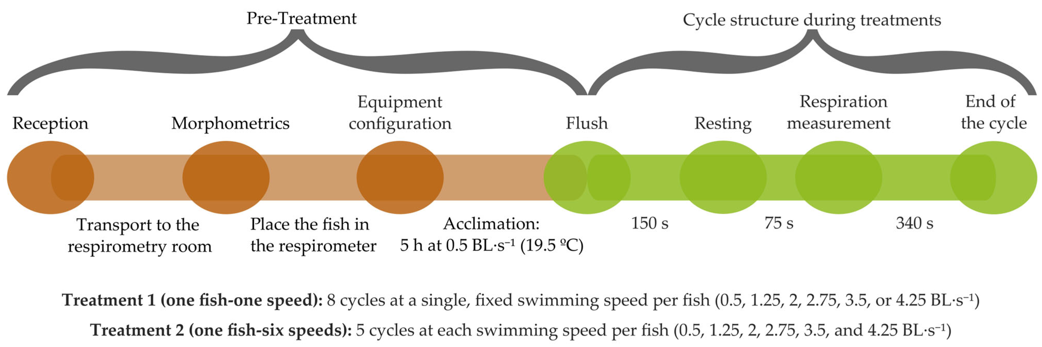
Two experimental treatments were designed (Figure 3). In treatment 1 (T1), respiration was measured at a single swimming speed (0.5, 1.25, 2, 2.75, 3.5, or 4.25 BL·s⁻¹), one fish and one velocity. The maximum velocity was chosen as fish speed in the ocean during diel vertical migration is always below this value [13]. In treatment 2 (T2), respiration was measured across the same six increasing swimming speeds, but with one fish and six velocities. Every fish in treatment T2 was labelled as Ramp 1, 2 or 3 to indicate that it underwent a progressive sequence of swimming speeds. After the acclimation time, eight cycles of 150 s flushing periods, followed by 75 s resting period and 340 s respiration measurement, were performed for each swimming speed in T1, while five cycles of flushing (150 s), resting (75 s), and measurement (340 s) cycles were performed in the T2 (30 cycles in total). The number of cycles in T2 was reduced compared to T1 in order to avoid the activation of anaerobic metabolism at higher swimming speeds as a result of prolonged physical effort (more than 200 min). Svendsen et al. [39] calculated that the maximal swimming speed for a sustained swimming without fatigue was 40 cm·s⁻¹ for sea bream (15 cm length) at 10 °C. In our procedure (12 cm length and 19.5 °C), the sustained swimming speed was ≈3.3 BL·s⁻¹, but the duration at which the animal was exposed to higher speeds was reduced to 94.2 min, as the metabolic activity should be higher in our higher-temperature conditions. Three replicates were performed for each swimming speed in T1, and three fish were used for T2. Oxygen saturation level was maintained above 80% by the end of the measurement period to avoid hypoxia [40].

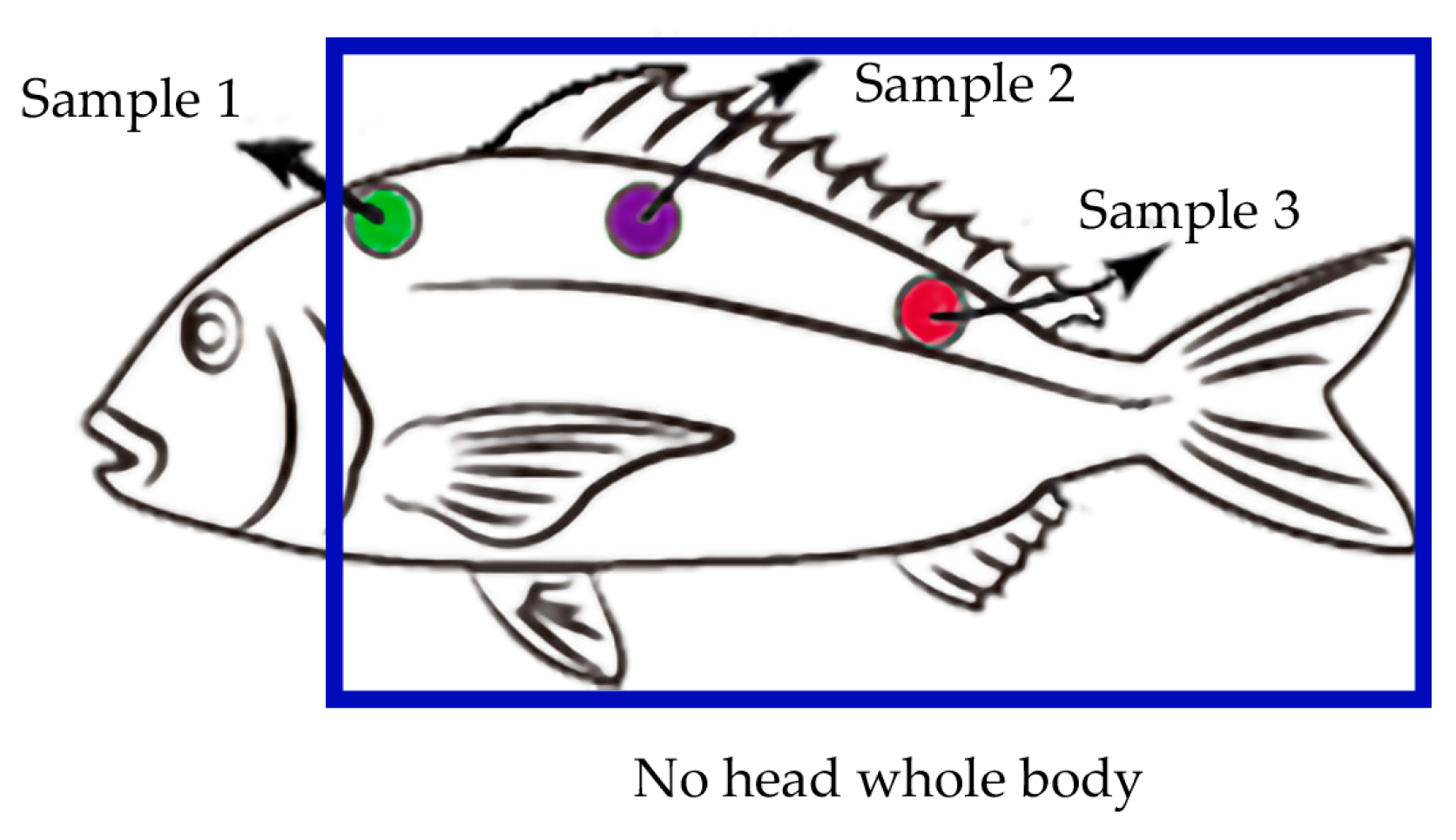
After euthanasia, three muscle samples were collected from each fish for ETS activity analysis with the aim of studying differences along the fish body: one near the head (Sample 1), one at mid-body (Sample 2), and one near the tail (Sample 3), all above the lateral line (Figure 4), avoiding organs and ensuring full muscle tissue. These samples and the remaining body (excluding the head) were frozen in liquid nitrogen and stored at −80 °C.

MO₂ values originally expressed in mg O₂ were converted to µL O₂ using oxygen density at experimental temperature with the Engineering ToolBox oxygen density calculator [41]. Finally, MO₂ values were expressed per mg of dry mass (DM) by converting the initially measured WM into DM using the DM/WM ratio of 0.23 [42] for fish, which is consistent with the values reported by Childress and Nygaard [43].

Based on the expected physiological response of fish to increasing swimming speed, we hypothesized that the relationship between MO₂ and swimming speed follows a four-parameter sigmoidal model:

$${\mathrm{M}\mathrm{O}}_2=\mathrm{d}+{\displaystyle \frac{\mathrm{a}-\mathrm{d}}{1+{\mathrm{e}}^{\left(-\mathrm{b}·\left(\mathrm{S}\mathrm{w}\mathrm{i}\mathrm{m}\mathrm{m}\mathrm{i}\mathrm{n}\mathrm{g}\mathrm{s}\mathrm{p}\mathrm{e}\mathrm{e}\mathrm{d}-\mathrm{c}\right)\right)}}}$$

(1)

where a is the upper asymptote (maximum MO₂), b is the slope between asymptotes (rate of change in MO₂ with swimming speed), c is the inflexion point (the swimming speed at which MO₂ reaches 50% of its maximum value and begins to increase rapidly), and d is the lower asymptote (minimum MO₂). At 0 BL·s⁻¹, MO₂ corresponds to the lower asymptote of the curve, representing the minimal metabolic demand required to sustain life. As swimming speed increases, MO₂ rises progressively until it approaches a maximal value (the upper asymptote) beyond which further increases in activity can no longer be supported by aerobic metabolism alone; we refer to this limit as the maximal aerobic capacity.

2.4. ETS Activity

Frozen samples were homogenized in Trizma (Sigma-Aldrich, St. Louis, MO, USA, T1503) medium (pH 7.8) using a Potter-Elvehjem homogenizer (glass vessel and PTFE plunger, Labbox Labware S.L., Premia de Dalt, Spain) and analyzed according to the method of Packard [44] modified for fish ETS assays according to Ariza et al. [19]. ETS activity was measured at 18.6 ± 0.6 °C (standard deviation). An activation energy of 15 kcal·mol⁻¹ was used in the Arrhenius equation to make temperature corrections [45]. ETS activity (µL O₂·mg protein⁻¹·h⁻¹) was calculated by quantifying protein content using the Lowry method [46], modified by Rutter [47]. To compare ETS activity with MO₂ values obtained from respirometry, protein biomass was converted to dry mass (DM) using a DM/protein ratio of 2.21, as reported for fish [48].

2.5. Statistical Analysis

Statistical analyses were performed using SPSS Statistics 22.0.0 (IBM Corp., Armonk, NY, USA) [49] and R software (version 4.4.3; R Core Team, 2025) [50]. Non-parametric tests were applied in general due to the lack of normality in several datasets, as confirmed by Shapiro–Wilk tests.

Differences in MO₂ among individuals at each swimming speed within T1 and between T1 and T2 were assessed using Kruskal–Wallis tests. For T2, Friedman tests were applied to evaluate intra-individual differences in MO₂ across swimming speeds in Ramps 2 and 3, followed by Wilcoxon signed-rank tests for pairwise comparisons when appropriate. For Ramp 1, a repeated-measures ANOVA with Greenhouse–Geisser correction (p < 0.001) was performed, followed by paired-samples t-tests. MO₂ was analyzed using an REML linear mixed-effects model with treatment and swimming speed as fixed effects, and a random intercept for fish.

Spearman correlation analyses were conducted to explore the relationship between ETS activity and swimming speed in T1, between ETS activity and physical characteristics of the fish (wet mass, length, width, and height), and between ETS activity and R/ETS ratios across sampling zones. Differences in ETS activity between treatments were assessed using Mann–Whitney U test and Friedman test followed by Wilcoxon signed-rank test among sampling positions for pair comparisons.

To model the relationship between MO₂ and swimming speed as well as between R/ETS and swimming speed, a four-parameter sigmoidal regression was fitted using nonlinear least squares in R. Individual fits were performed using the nlsLM function from the minpack.lm package 1.2-4 [51]. Mixed-effects models were implemented using the saemix package 3.4 [52] to account for population-level models. Model performance was evaluated using pseudo-R², AIC, and BIC values (full statistical details of fits are provided in Tables S2 and S3). All parameters were tested for statistical significance, and residual diagnostics were performed to assess model validity. Graphical representations were generated using the ggplot2 package 4.0.1 [53].

3. Results

3.1. Respirometry

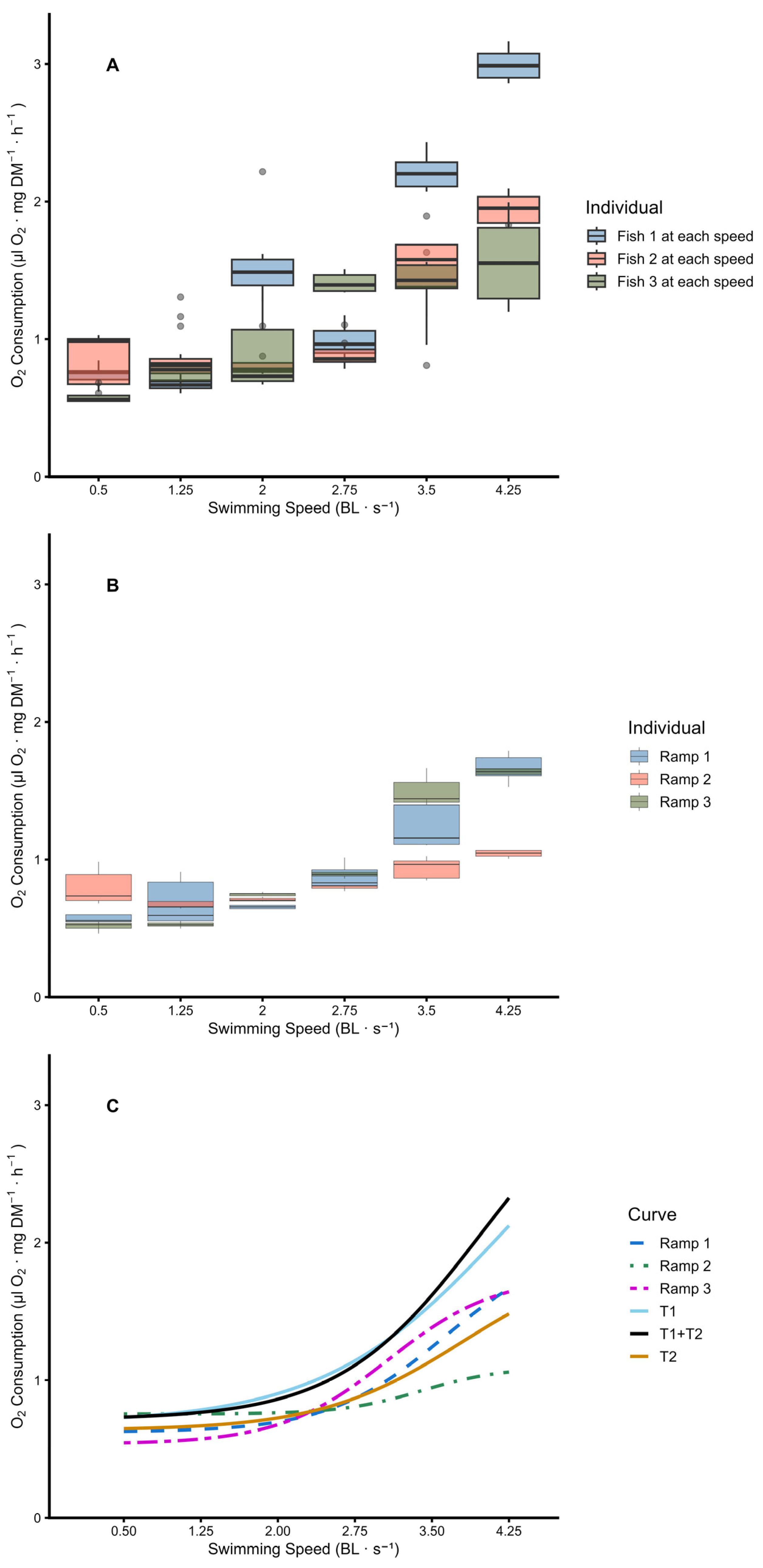
In T1, the experimental design prevented intra-individual analysis. Inter-individual comparisons of the rate of oxygen consumption at each swimming speed revealed similar values at 1.25 BL·s⁻¹ (Kruskal–Wallis test, p = 0.086, Table S4), but significant differences at other speeds (p < 0.05), thus indicating rather high variability among individuals (Figure 5A). A four-parameter sigmoidal model fitted using a nonlinear mixed-effects approach (Figure 5C) explained 61.7% of the variability in oxygen consumption (Pseudo-R² = 0.617). The estimated parameters (

Table 1. Estimated parameters (±standard error) of the four-parameter sigmoidal model fitted to the relationship between swimming speed and metabolic response. Two fitting approaches were used: SAEMIX (Stochastic Approximation Expectation-Maximization) for population-level models (T1, T2, and combined T1 + T2), and nlsLM (nonlinear least squares using Levenberg–Marquardt algorithm) for individual fish (labelled as Ramp 1–3). For the combined dataset (T1 + T2), the model was fitted using SAEMIX with covariates to account for treatment effects. Parameters: a (upper asymptote), b (slope), c (inflexion point), and d (lower asymptote). Pseudo-R² indicates goodness of fit. Residual Error reflects the standard deviation of residuals for individual models, providing an estimate of within-model variability.

Parameter	T1 (SAEMIX)	T2 (SAEMIX)	T1 + T2 (SAEMIX + Cov)	Ramp 1 (nlsLM)	Ramp 2 (nlsLM)	Ramp 3 (nlsLM)
a (±SE) μL O2·kg DM−1·h−1	3.558 ± 2.003	1.925 ± 0.436	3.398 ± 1.215	2.009 ± 0.410	1.094 ± 0.121	1.762 ± 0.143
b (±SE) BL·s−1	1.114 ± 0.607	1.443 ± 0.386	1.443 ± 0.639	1.768 ± 0.678	2.563 ± 2.180	1.892 ± 0.520
c (±SE) BL·s−1	4.248 ± 1.357	3.801 ± 0.423	3.969 ± 0.782	3.622 ± 0.390	3.402 ± 0.407	3.074 ± 0.169
d (±SE) μL O2·kg DM−1·h−1	0.686 ± 0.100	0.637 ± 0.034	0.715 ± 0.059	0.623 ± 0.051	0.755 ± 0.033	0.536 ± 0.053
Pseudo-R2	0.617	0.719	0.874 (population) −4.75 (individual)	0.908	0.562	0.927
Residual Error	—	—	—	0.130	0.110	0.126

) showed coefficients of variation ranging from 14.5% to 56.3% (Table S2).

In T2 (Figure 5B), the intra-individual analysis showed no significant differences in oxygen consumption at low swimming speeds (0.5, 1.25, and 2 BL s⁻¹) (paired t-test, p > 0.05, Table S5), but differences at higher speed (2.75, 3.5, and 4.25 BL s⁻¹) for Ramp 1 (p < 0.05). For Ramp 2, there were no differences between 0.5 and 1.25 BL·s⁻¹, between 2.0 and 2.75 BL·s⁻¹, or between 1.25 and 2.0/2.75 BL·s⁻¹ (all p > 0.05), but we observed a borderline difference for 1.25 vs. 3.5 BL·s⁻¹ (p = 0.08) and 1.25 vs. 4.25 BL·s⁻¹ (p = 0.08). However, we found differences among 2, 2.75, 3.5 and 4.25 BL·s⁻¹ (p < 0.05). Ramp 3 showed significant differences across speeds except between 0.5 and 1.25 BL s⁻¹ and between 3.5 and 4.25 BL·s⁻¹ (Wilcoxon test, p > 0.05, Table S7). For inter-individual analysis, individual sigmoidal models fitted (Figure 5C) to each fish yielded significant parameters (p < 0.05, Table 1), except for parameter b in Ramp 2 (p = 0.25). Model fit was high for Ramp 1 and 3 (Pseudo-R² > 0.90), but lower for Ramp 2 (Pseudo-R² < 0.60), which also showed a higher d value. Coefficients of variation across individuals were 23.8% for a, 16.8% for b, 14.1% for d, and 6.7% for c (Table S2), indicating substantial variability in a, b, and d, and therefore substantial inter-individual variability. For this reason, we applied a nonlinear mixed-effects approach to the T2 data (Table 1). This model explains 71.9% of the variability (Pseudo-R² = 0.719), with coefficients of variation ranging from 5.3% to 26.7% (Table S2).

We assessed the influence of treatment on MO₂ using a linear mixed-effects model (Table S8), finding no significant effect (p = 0.119). Accordingly, a combined sigmoidal model including both treatments as covariates was fitted to assess systematic differences (Table 1). At the population level (without individual variability), the model performed poorly (Pseudo-R² = −4.75) and no covariate effects were significant (p > 0.05, Table S2). However, when individual variability was included, the model explained 87.4% of the total variability (Pseudo-R² = 0.874), outperforming the separate models. Coefficients of variation ranged from 8.3% to 44.3%. AIC and BIC values were lower than those found in T1 but higher than in T2 (Table S2), suggesting the combined model improves over T1 but not over T2. Across models, parameters a, b, and c showed higher variability than d, indicating large uncertainty in estimating the asymptote, slope, and inflexion point. These results support the use of a unified sigmoidal model to describe the oxygen consumption across treatments.

3.2. ETS Activity

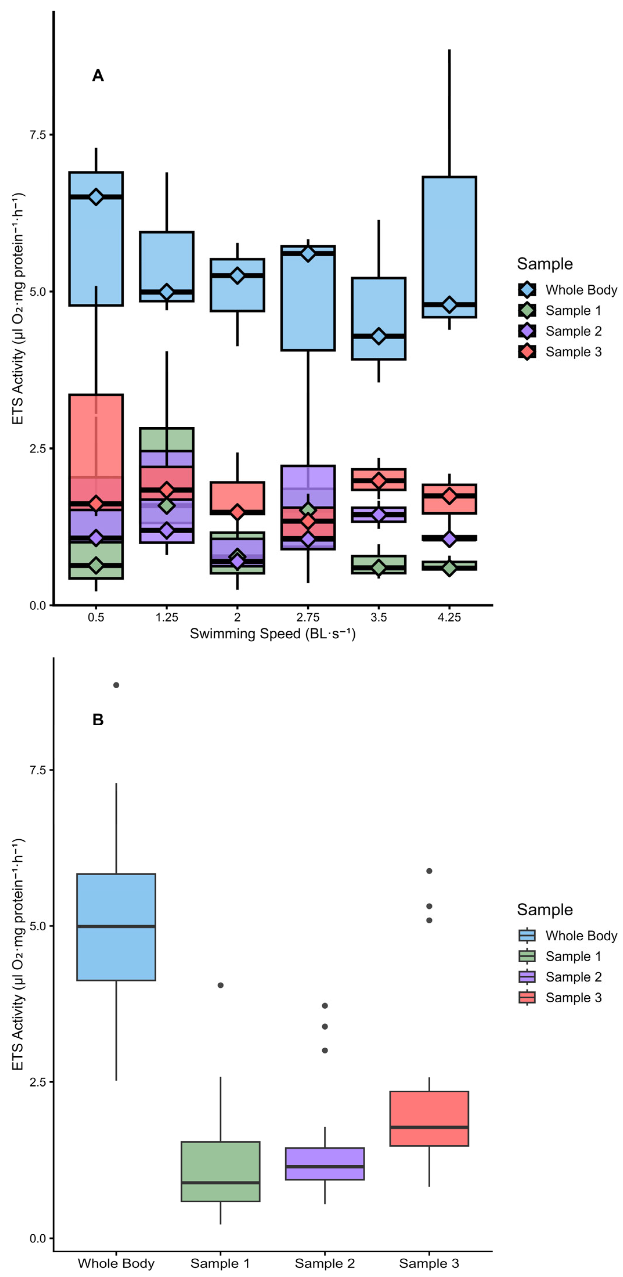
We did not find a correlation between ETS activity values and swimming speed in T1 (Figure 6A, Spearman test, p > 0.050, Table S9). However, there was a significant correlation among samples 1, 2 and 3 (p < 0.05). A comparison of the ETS activity profile (whole-body and localized muscle samples 1, 2 and 3) between treatments revealed differences only in sample 3 (Mann–Whitney test, p < 0.05, Table S10). We also observed differences in the ETS activity profile (Figure 6B, Friedman test, p < 0.05, Table S11), except between samples 1 and 2 (Wilcoxon test, p = 0.085, Bonferroni-adjusted p-value = 0.008, Table S12). There was no correlation between whole-body ETS activity and fish physical traits (mass, length, width and height; Spearman test, p > 0.05, Table S13). However, sample 3 correlated with all traits except body width (p < 0.05), sample 1 correlated with length, and sample 2 showed borderline correlation (p = 0.053). We applied a multiple linear regression model to assess proportionality between whole-body ETS and localized samples. The model was not significant (R² = 0.102, p > 0.05, Table S14).

3.3. Respiration/ETS Activity Relationship

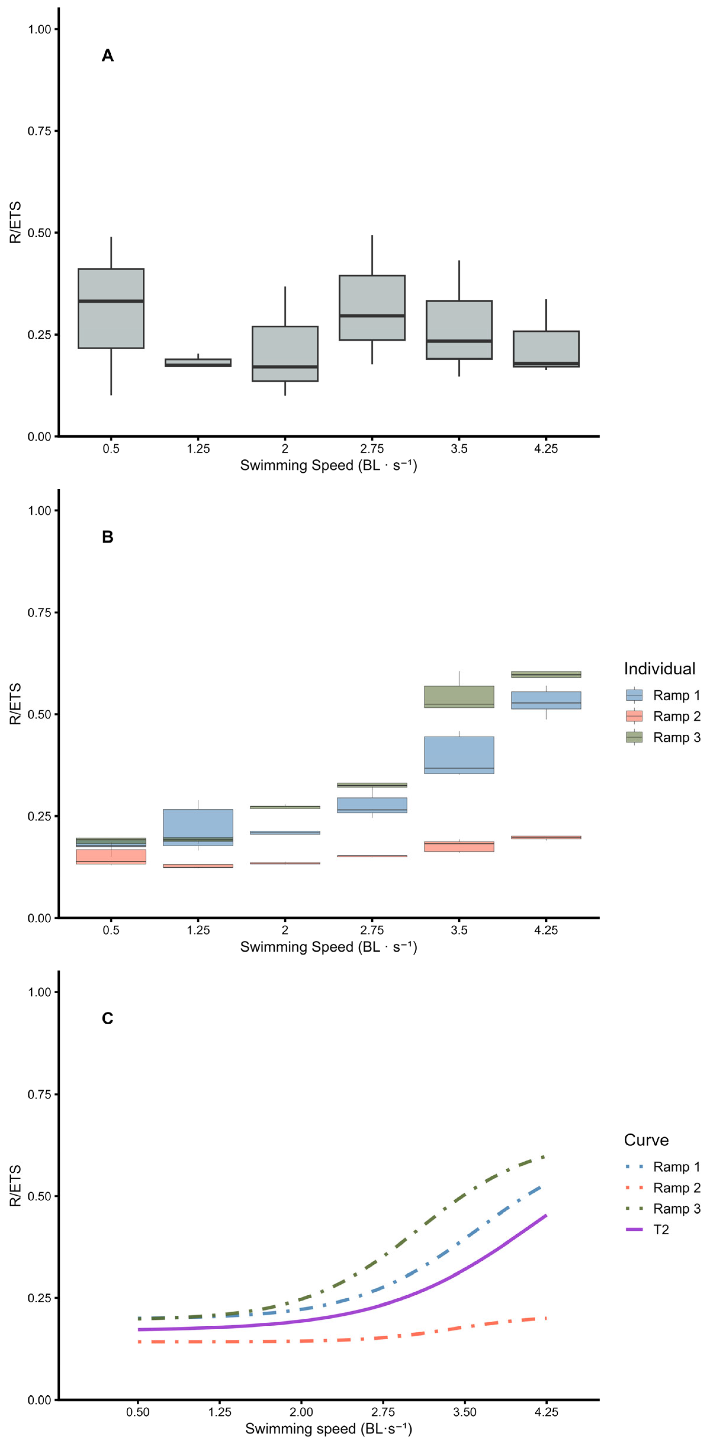
In T1, normalizing oxygen consumption by whole-body ETS activity (R/ETS) removed dependence on swimming speed (Figure 7A, Kruskal–Wallis test, p = 0.812, Table S15). Relative variability among fish was high (mean R/ETS coefficient of variation at each speed ranged from 42.4 to 65.1%) except at 1.25 BL·s⁻¹ (CV = 9.5%).

In T2 (Figure 7B), R/ETS values at each swimming speed showed intra-individual differences (Wilcoxon test, p < 0.05, Table S16). Ramp 1 showed no differences among low swimming speeds (p > 0.05), but differences occurred between low and high speeds and among higher swimming speeds (p < 0.05). Ramp 2 showed no differences at lower and intermediate speeds (p > 0.05), but differences appeared between intermediate and high speeds and among higher speeds (p < 0.05). Ramp 3 showed differences across all speeds except among higher ones (p = 0.08). Inter-individual comparisons revealed significant differences at all speeds except at 0.5 and 1.25 BL·s⁻¹ (Kruskal–Wallis test, p > 0.05, Table S17).

Individual four-parameter sigmoidal models fitted to R/ETS data (Figure 7C,

Table 2. Estimated parameters (±standard error) of the four-parameter sigmoidal model fitted to the relationship between swimming speed and R/ETS ratio. Individual models (for T2 fishes labelled Ramp 1–3) were fitted using nlsLM (nonlinear least squares with Levenberg–Marquardt algorithm), while the population-level model (T2) was fitted using SAEMIX (Stochastic Approximation Expectation-Maximization). Parameters: a (upper asymptote), b (slope), c (inflexion point), and d (lower asymptote). Pseudo-R² indicates goodness of fit; Residual Error reflects the standard deviation of residuals for individual models.

Parameter	Ramp 1 (nlsLM)	Ramp 2 (nlsLM)	Ramp 3 (nlsLM)	T2 (SAEMIX)
a (±SE)	0.641 ± 0.131	0.207 ± 0.024	0.642 ± 0.052	0.707 ± 0.067
b (±SE) BL·s−1	0.567 ± 0.217	0.396 ± 0.340	0.529 ± 0.146	1.408 ± 0.246
c (±SE) BL·s−1	3.623 ± 0.390	3.412 ± 0.421	3.076 ± 0.169	4.168 ± 0.673
d (±SE)	0.198 ± 0.016	0.143 ± 0.006	0.195 ± 0.019	0.169 ± 0.013
Pseudo-R2	0.908	0.563	0.927	0.442
Residual Error	0.041	0.021	0.046	—

) showed significant parameters (p < 0.05, Table S3) except for parameter b in Ramp 2 (p = 0.255). Model fit was high for Ramp 1 and Ramp 3 (Pseudo-R² > 0.90) and lower for Ramp 2 (Pseudo-R² = 0.56). Ramp 2 showed a lower upper asymptote (a), a non-significant slope parameter (b), and reduced goodness of fit. Coefficients of variation across fish were 50.5% for a, 18.0% for b, 7.6% for c, and 17.3% for d, indicating high variability in maximum R/ETS (a), moderate variability for slope (b), and minimum R/ETS (d), and a consistent point of inflexion (c) among fish. We fitted a nonlinear mixed-effects model using a four-parameter sigmoidal function to describe the R/ETS–swimming speed relationship under treatment T2 (Figure 7C, Table 2). We found coefficients of variation ranging from 7.94% to 17.47% (Table S3), indicating a rather good estimation of the parameter. However, the population-level Pseudo-R² was 0.44, indicating moderate explanatory power. Individual-level Pseudo-R² was negative, showing limited improvement from random effects. These results reveal different patterns between treatments precluding a unified model combining T1 and T2.

4. Discussion

Respirometry confirmed that MO₂ in juvenile gilthead sea bream follows a four-parameter sigmoidal relationship with swimming speed (Figure 5C), consistent with the expected transition from routine metabolism to maximal aerobic capacity. At low swimming speeds (0.5 to 2 BL·s⁻¹), MO₂ remained relatively stable, suggesting that fish were swimming comfortably against the current without engaging in free movement. When speed increased to intermediate levels (2.75 to 3.5 BL·s⁻¹), MO₂ rose sharply, reflecting the onset of sustained physical effort. At higher speeds (>3.5 BL·s⁻¹) the increase became moderate until reaching a maximum value. Fish exhibited different responses at the same speeds, indicating a high inter-individual variability (Figure 5A,B). This variability likely reflects differences in physical capacity and swimming efficiency among individuals. At lower speeds, fish could move freely within the chamber, contributing to behavioural variability, whereas intermediate speeds required continuous swimming effort, reducing behavioural freedom and revealing differences in physical performance as speed gradually increases. We interpret this variability as natural; however, in some cases, the maximal diel activity period was exceeded due to experimental constraints, potentially introducing additional variability (particularly in T2 at higher speeds). To minimize this, future protocols should initiate measurements at the beginning of the diel activity peak. Although the T2 model showed a better fit than T1 (Table 1), the different treatments did not promote systematic changes in the shape of the MO₂ curve (Figure 5C), nor there was any influence of treatment on MO₂ (Table S8). Therefore, we unified both datasets to derive a general relationship applicable to gilthead sea bream within the size range and maturity used in this study (Table 1). Although the unified model showed a worse fit than T2, its broader data coverage makes it more suitable for estimating MO₂ under natural conditions.

Based on T1, we observed that swimming activity did not induce immediate changes in the specific ETS activity (Figure 6A), suggesting that ETS is independent of the short-term metabolic activity level and supports its use as a proxy for potential oxygen consumption ability. ETS activity results in a stable reference capacity to normalize oxygen consumption. We observed no relationship between ETS activity and physical traits (Table S13), although a larger dataset including fish at different maturity stages is needed to confirm this observation.

We were unable to identify a representative subsample for ETS activity. Samples 1, 2 and 3 showed lower ETS values compared to whole-body measurements and did not correlate with them (Figure 6B). However, sample 3 exhibited significantly higher ETS activity than samples 1 and 2 (Table S12), possibly due to its anatomical location near the tail, where red muscle from the lateral line is included. Red muscle is associated with aerobic swimming and contains a higher mitochondrial density than white muscle, resulting in greater ETS activity per unit mass [54]. Teulier et al. [55] found that red muscle contributes disproportionately to total muscle oxidative metabolism (58%), despite representing less than 5% of total muscle mass in gilthead sea bream. This could explain the elevated ETS activity in sample 3 and suggests that red muscle may account for a substantial portion of the whole-body ETS signal. Thoral et al. [56] demonstrated a non-lethal sampling of red muscle that does not affect metabolic rate or swimming performance. Therefore, investigating the relationship between whole-body ETS and red muscle ETS could prevent the entire animal being consumed in one assay, enable the non-lethal estimation of metabolic capacity, and allow the same individuals to be used in longitudinal studies. In our study, whole-body samples included highly oxidative organs such as the liver and heart, which likely contributed to the overall ETS value. Future research should quantify the contribution of individual organs to ETS activity and assess whether excluding the head (which contains the brain and gills) affects whole-body ETS activity estimates. Also, we must note that the effect of the anesthetic MS-222 on ETS activity determination is still unknown.

Normalizing MO₂ by ETS activity preserved the four-parameter sigmoidal relationship with swimming speed only in T2 (Figure 7B,C). In contrast, the independence of ETS activity from swimming speed, combined with the high inter-individual variability in T1, invalidates any consistent relationship between the R/ETS ratio and speed in this treatment (Figure 7A), and therefore invalidates pool T1 and T2 for modelling an activity-dependent R/ETS. In T1, the lack of correlation may be partly due to the experimental design, where each fish was exposed to a single swimming speed. Individual sigmoidal models (Table 2) revealed that the slope was the most difficult parameter to estimate, particularly in Ramp 2, where it was not statistically significant and exhibited high variability (Table S3). In contrast, the inflexion point (ranging from 3.08 to 3.62 BL·s⁻¹) and the lower asymptote (0.14–0.20) were more consistent across individuals. The upper asymptote (parameter a) exhibited substantial inter-individual variability, with values of 0.64 for Ramps 1 and 3, and a markedly lower value of 0.21 for Ramp 2 (CV across fish = 50%). To explore a common pattern, a single model was fitted to all T2 fish (Figure 7C). Despite the divergent behaviour of Ramp 2 and the limited sample size, the model moderately explained the variability (Pseudo-R² = 0.44, Table 2) and displayed a steeper slope than the individual fits, as well as a higher inflexion point. Nevertheless, parameter d (0.17) was consistent with the individual models, and parameter a (0.71) aligned more closely with Ramps 1 and 3 than with Ramp 2. Assuming this model is representative of T2, MO₂ would range from 0.17 ± 0.01 to 0.71 ± 0.07 relative to ETS activity depending on swimming speed.

Accordingly, the R/ETS ratio could be interpreted as the fraction of the maximal mitochondrial oxygen-processing capacity being used at a given activity level. Since the respiration rate ranges from the vital-maintenance levels to values approaching the maximal aerobic capacity, it follows that 0 < R/ETS < 1. The upper bound reflects that physiological conditions cannot match the ETS non-limiting conditions. Applying this model to micronekton fish suggests that during the initial phase of diel vertical migration, starved individuals may operate at approximately 17% of their ETS activity, whereas active feeding or escape responses in shallower layers could reach up to 71%. However, these extrapolations should be interpreted with caution, as they do not account for species-specifics morphology, swimming behaviour, or temperature effects, which may substantially alter R/ETS ratios. Further R/ETS measurements in more representative micronektonic species are needed to establish a general R/ETS ratio. Our estimates were obtained under fasting conditions, minimizing the influence of digestion on MO_2, so the MO₂ could be related to the total aerobic metabolism [36]. Thus, its application to a non-post absorptive state, such as when animal remain at depth digesting, needs further research.

Traditionally, a conservative R/ETS ratio of 0.5 has been used to estimate respiratory fluxes [57]. Assuming a sustained swimming speed of 2 BL·s⁻¹, which marks the onset of increased MO₂ [39], the R/ETS ratio would be 0.19 ± 0.03 (lower than the conventional value). Using the inflexion point of the model as the threshold for accelerated MO₂, the R/ETS ratio would be 0.44 ± 0.13, closer to the traditional estimate. However, Barham [58] described the daytime activity of myctophids at depth as static, suggesting that a ratio of 0.19 ± 0.03 may be more appropriate for estimating respiration and carbon remineralization at depth. Christiansen et al. [59] reported that Maurolicus muelleri exhibited slow and short vertical movements while they stay at depth at 0.5–2.5 cm·s⁻¹ (<1 BL·s⁻¹), and faster vertical motion at speeds up to 15–20 cm·s⁻¹. Assuming a mean body length of 2.5 cm, these fish would have R/ETS ratios ranging from 0.17 ± 0.01 (at 0.2–1 BL·s⁻¹) to 0.67 ± 0.07 and 0.70 ± 0.07 (at 6–8 BL·s⁻¹). To apply a reliable R/ETS ratio, it is essential to determine the proportion of time that fish spend at different activity levels. At depth, a ratio of 0.17–0.19 seems appropriate for resting individuals. Thus, higher values (0.44–0.70) should be applied during vertical migration below the mixed layer and in their feeding ground at the epipelagic zone. Intermediate ratios may be applicable during daytime residence depth in animals that are in an absorptive state. However, digestion time and gut evacuation rates should be studied in order to determine the most appropriate ratio.

Temperature is a key determinant of metabolic processes and must be considered when extrapolating R/ETS ratios to natural conditions. ETS activity should be corrected using Arrhenius-type adjustments, but the activation energies for micronekton remain unknown, introducing uncertainty. Clarke and Johnston [60] showed that teleost metabolic rates follow an Arrhenius relationship, while Killen et al. [61] provided predictive models integrating body mass and temperature, offering alternatives to simple Q₁₀ corrections. Belcher et al. [62] proposed an allometric equation for MO₂ based on respirometry and ETS-derived estimates, yet these equations rely on assumed activation energies and a fixed ETS-to-respiration ratio. Moreover, Alewijnse et al. [63] showed that oxygen consumption estimates differ substantially among methods (otolith proxies, allometric models, ETS), underscoring the need for direct validation. Future work should include controlled swimming respirometry across a range of temperatures to derive species-specific MO₂–speed relationships, enabling accurate R/ETS calculations under realistic thermal conditions and improving predictions of aerobic performance and carbon flux in micronekton.

5. Conclusions

This study demonstrates that MO₂ in juvenile gilthead sea bream follows a four-parameter sigmoidal relationship with swimming speed, reflecting distinct phases of metabolic response to increasing physical effort. While both treatments (T1 and T2) allowed for model fitting, the T2 treatment yielded more consistent results, enabling the construction of a model for estimating aerobic metabolism across swimming speeds. However, given the limited sample size and observed inter-individual variability, this model should be considered a preliminary representation of the trend rather than a precise predictive tool. The independence of ETS activity from short-term swimming effort supports its use as a proxy for maximal aerobic capacity. However, localized muscle did not reliably reflect whole-body ETS activity, likely due to the predominance of white muscle, which is primarily involved in anaerobic performance. Although sample 3 showed elevated ETS activity (likely reflecting the presence of red muscle fibres) this was not consistent across individuals. These findings underscore the need to identify anatomical regions with ETS activity comparable to whole-body measurements, which would enable non-lethal sampling methods and preserve individual fish for collection, morphometry, and other studies.

The normalization of MO₂ by ETS activity (R/ETS ratio) preserved the sigmoidal relationship with swimming speed only in T2, suggesting that this ratio may reflect changes in aerobic effort relative to the maximal capacity of the organism. According to this model, aerobic metabolism should range from 17% to 71% of their ETS activity depending on swimming speed. Considering observed swimming behaviours and diel vertical migration patterns, the traditional use of a conservative R/ETS ratio of 0.5 to estimate active carbon flux may need to be reconsidered. Lower ratios (0.17–0.19) may better represent metabolic activity during quiescent phases at depth, while it could increase if animals are in an absorptive state. Higher ratios (0.44–0.70) would be more appropriate during active vertical movements and during feeding in shallower layers. Incorporating this variability into biogeochemical models could improve estimates of carbon remineralization mediated by micronekton. Operationally, future active-flux estimates could be obtained by (i) measuring ETS, (ii) using R/ETS ratios to determine the specific R value at each activity level, (iii) weighting by residence time below the mixed layer, and (iv) applying temperature corrections to obtain a more realistic remineralization rate at depth. However, the morphological and physiological differences between juvenile gilthead sea bream and micronekton fish underscore the need to validate the robustness of these conclusions using ecologically relevant fish models.

References

1. Ciais, P.; Sabine, C.; Bala, G.; Bopp, L.; Brovkin, V.; Canadell, J.; Chhabra, A.; DeFries, R.; Galloway, J.; Heimann, M.M.; et al. Carbon and Other Biogeochemical Cycles. In Climate Change 2013 the Physical Science Basis: Working Group I Contribution to the Fifth Assessment Report of the Intergovernmental Panel on Climate Change; Stocker, T.F., Qin, D., Plattner, G.-K., Tignor, M., Allen, S.K., Boschung, J., Nauels, A., Xia, Y., Bex, V., Midgley, P.M., Eds.; Cambridge University Press: Cambridge, UK; New York, NY, USA, 2013; pp. 465–570. [Google Scholar]
2. Honjo, S.; Eglinton, T.; Taylor, C.; Ulmer, K.; Sievert, S.; Bracher, A.; German, C.; Edgcomb, V.; Francois, R.; Iglesias-Rodriguez, M.D.; et al. Understanding the Role of the Biological Pump in the Global Carbon Cycle: An Imperative for Ocean Science. Oceanography 2014, 27, 10–16. [Google Scholar] [CrossRef]
3. Ducklow, H.W.; Steinberg, D.K.; Buesseler, K.O. Upper Ocean Carbon Export and the Biological Pump. Oceanography 2001, 14, 50–58. [Google Scholar] [CrossRef]
4. Volk, T.; Hoffert, M.I. Ocean Carbon Pumps: Analysis of Relative Strengths and Efficiencies in Ocean-Driven Atmospheric CO2 Changes. The Carbon Cycle and Atmospheric CO2: Natural Variations Archean to Present; American Geophysical Union: Washington, DC, USA, 1985; pp. 99–110. [Google Scholar]
5. Legendre, L.; Rivkin, R.B.; Weinbauer, M.G.; Guidi, L.; Uitz, J. The Microbial Carbon Pump Concept: Potential Biogeochemical Significance in the Globally Changing Ocean. Prog. Oceanogr. 2015, 134, 432–450. [Google Scholar] [CrossRef]
6. Jiao, N.; Robinson, C.; Azam, F.; Thomas, H.; Baltar, F.; Dang, H.; Hardman-Mountford, N.J.; Johnson, M.; Kirchman, D.L.; Koch, B.P.; et al. Mechanisms of Microbial Carbon Sequestration in the Ocean—Future Research Directions. Biogeosciences 2014, 11, 5285–5306. [Google Scholar] [CrossRef]
7. Jiao, N.; Herndl, G.J.; Hansell, D.A.; Benner, R.; Kattner, G.; Wilhelm, S.W.; Kirchman, D.L.; Weinbauer, M.G.; Luo, T.; Chen, F.; et al. Microbial Production of Recalcitrant Dissolved Organic Matter: Long-Term Carbon Storage in the Global Ocean. Nat. Rev. Microbiol. 2010, 8, 593–599. [Google Scholar] [CrossRef] [PubMed]
8. Planton, S. (Ed.) IPCC Annex III: Glossary. In Climate Change 2013: The Physical Science Basis. Contribution of Working Group I to the Fifth Assessment Report of the Intergovernmental Panel on Climate Change; Cambridge University Press: Cambridge, UK, 2013; pp. 1447–1466. [Google Scholar] [CrossRef]
9. Ricour, F.; Guidi, L.; Gehlen, M.; DeVries, T.; Legendre, L. Century-Scale Carbon Sequestration Flux throughout the Ocean by the Biological Pump. Nat. Geosci. 2023, 16, 1105–1113. [Google Scholar] [CrossRef]
10. Buesseler, K.O.; Antia, A.N.; Chen, M.; Fowler, S.W.; Gardner, W.D.; Gustafsson, O.; Harada, K.; Michaels, A.F.; Rutgers van der Loeff, M.; Sarin, M.; et al. An Assessment of the Use of Sediment Traps for Estimating Upper Ocean Particle Fluxes. J. Mar. Res. 2007, 65, 345–416. [Google Scholar] [CrossRef]
11. Le Moigne, F.A.C. Pathways of Organic Carbon Downward Transport by the Oceanic Biological Carbon Pump. Front. Mar. Sci. 2019, 6, 634. [Google Scholar] [CrossRef]
12. Bianchi, D.; Mislan, K.A.S. Global Patterns of Diel Vertical Migration Times and Velocities from Acoustic Data. Limnol. Oceanogr. 2016, 61, 353–364. [Google Scholar] [CrossRef]
13. Ariza, A.; Landeira, J.M.; Escánez, A.; Wienerroither, R.; Aguilar de Soto, N.; Røstad, A.; Kaartvedt, S.; Hernández-León, S. Vertical Distribution, Composition and Migratory Patterns of Acoustic Scattering Layers in the Canary Islands. J. Mar. Syst. 2016, 157, 82–91. [Google Scholar] [CrossRef]
14. Davison, P.C.; Checkley, D.M.; Koslow, J.A.; Barlow, J. Carbon Export Mediated by Mesopelagic Fishes in the Northeast Pacific Ocean. Prog. Oceanogr. 2013, 116, 14–30. [Google Scholar] [CrossRef]
15. Robinson, C.; Steinberg, D.K.; Anderson, T.R.; Arístegui, J.; Carlson, C.A.; Frost, J.R.; Ghiglione, J.-F.; Hernández-León, S.; Jackson, G.A.; Koppelmann, R.; et al. Mesopelagic Zone Ecology and Biogeochemistry—A Synthesis. Deep Sea Res. Part II Top Stud. Oceanogr. 2010, 57, 1504–1518. [Google Scholar] [CrossRef]
16. Getzlaff, J.; Kriest, I. Impacts of Vertical Migrants on Biogeochemistry in an Earth System Model. Glob. Biogeochem. Cycles 2024, 38, e2023GB007842. [Google Scholar] [CrossRef]
17. Hernández-León, S.; Olivar, M.P.; Fernández de Puelles, M.L.; Bode, A.; Castellón, A.; López-Pérez, C.; Tuset, V.M.; González-Gordillo, J.I. Zooplankton and Micronekton Active Flux Across the Tropical and Subtropical Atlantic Ocean. Front. Mar. Sci. 2019, 6, 535. [Google Scholar] [CrossRef]
18. Hernández-León, S.; Franchy, G.; Moyano, M.; Menéndez, I.; Schmoker, C.; Putzeys, S. Carbon Sequestration and Zooplankton Lunar Cycles: Could We Be Missing a Major Component of the Biological Pump? Limnol. Oceanogr. 2010, 55, 2503–2512. [Google Scholar] [CrossRef]
19. Ariza, A.; Garijo, J.C.; Landeira, J.M.; Bordes, F.; Hernández-León, S. Migrant Biomass and Respiratory Carbon Flux by Zooplankton and Micronekton in the Subtropical Northeast Atlantic Ocean (Canary Islands). Prog. Oceanogr. 2015, 134, 330–342. [Google Scholar] [CrossRef]
20. Dam, H.G.; Peterson, W.T. The Effect of Temperature on the Gut Clearance Rate Constant of Planktonic Copepods. J. Exp. Mar. Biol. Ecol. 1988, 123, 1–14. [Google Scholar] [CrossRef]
21. Clarke, T.A. Feeding Habits of Stomiatoid Fishes From Hawaiian Waters. Fish. Bull. 1982, 80, 287–304. [Google Scholar]
22. Baird, R.C.; Hopkins, T.L.; Wilson, D.F. Diet and Feeding Chronology of Diaphus Taaningi (Myctophidae) in the Cariaco Trench. Copeia 1975, 2, 356–365. [Google Scholar] [CrossRef]
23. Saba, G.K.; Steinberg, D.K. Abundance, Composition and Sinking Rates of Fish Fecal Pellets in the Santa Barbara Channel. Sci. Rep. 2012, 2, 7166. [Google Scholar] [CrossRef] [PubMed]
24. Longhurst, A.R.; Bedo, A.W.; Harrison, W.G.; Head, E.J.H.; Sameoto, D.D. Vertical Flux of Respiratory Carbon by Oceanic Diel Migrant Biota. Deep-Sea Res. Part A Oceanogr. Res. Pap. 1990, 37, 685–694. [Google Scholar] [CrossRef]
25. Dam, H.G.; Roman, M.R.; Youngbluth, M.J. Downward Export of Respiratory Carbon and Dissolved Inorganic Nitrogen by Diel-Migrant Mesozooplankton at the JGOFS Bermuda Time-Series Station. Deep-Sea Res. Part I Oceanogr. Res. Pap. 1995, 42, 1187–1197. [Google Scholar] [CrossRef]
26. del Giorgio, P.A.; Duarte, C.M. Respiration in the Open Ocean. Nature 2002, 420, 379–384. [Google Scholar] [CrossRef] [PubMed]
27. Hansen, A.N.; Visser, A.W. Carbon Export by Vertically Migrating Zooplankton: An Optimal Behavior Model. Limnol. Oceanogr. 2016, 61, 701–710. [Google Scholar] [CrossRef]
28. Pakhomov, E.A.; Podeswa, Y.; Hunt, B.P.V.; Kwong, L.E. Vertical Distribution and Active Carbon Transport by Pelagic Decapods in the North Pacific Subtropical Gyre. ICES J. Mar. Sci. 2019, 76, 702–717. [Google Scholar] [CrossRef]
29. Ikeda, T. Routine Metabolic Rates of Pelagic Marine Fishes and Cephalopods as a Function of Body Mass, Habitat Temperature and Habitat Depth. J. Exp. Mar. Biol. Ecol. 2016, 480, 74–86. [Google Scholar] [CrossRef]
30. Irigoien, X.; Klevjer, T.A.; Røstad, A.; Martinez, U.; Boyra, G.; Acuña, J.L.; Bode, A.; Echevarria, F.; Gonzalez-Gordillo, J.I.; Hernandez-Leon, S.; et al. Large Mesopelagic Fishes Biomass and Trophic Efficiency in the Open Ocean. Nat. Commun. 2014, 5, 3271. [Google Scholar] [CrossRef]
31. Saba, G.K.; Burd, A.B.; Dunne, J.P.; Hernández-León, S.; Martin, A.H.; Rose, K.A.; Salisbury, J.; Steinberg, D.K.; Trueman, C.N.; Wilson, R.W.; et al. Toward a Better Understanding of Fish-Based Contribution to Ocean Carbon Flux. Limnol. Oceanogr. 2021, 66, 1639–1664. [Google Scholar] [CrossRef]
32. Gómez, M.; Torres, S.; Hernández-León, S. Modification of the Electron Transport System (ETS) Method for Routine Measurements of Respiratory Rates of Zooplankton. S. Afr. J. Mar. Sci. 1996, 17, 15–20. [Google Scholar] [CrossRef]
33. Owens, T.G.; King, F.D. The Measurement of Respiratory Electron-Transport-System Activity in Marine Zooplankton. Mar. Biol. 1975, 30, 27–36. [Google Scholar] [CrossRef]
34. Ikeda, T. Estimated Respiration Rate of Myctophid Fish from the Enzyme Activity of the Electron-Transport-System. J. Oceanogr. Soc. Jpn. 1989, 45, 167–173. [Google Scholar] [CrossRef]
35. Loligo® Systems. AutoRespTM Software for Respirometry, Version 2.2.0; Loligo ® Systems A/S: Viborg, Denmark, 2016.
36. Chabot, D.; Steffensen, J.F.; Farrell, A.P. The Determination of Standard Metabolic Rate in Fishes. J. Fish Biol. 2016, 88, 81–121. [Google Scholar] [CrossRef] [PubMed]
37. Chabot, D.; McKenzie, D.J.; Craig, J.F. Metabolic Rate in Fishes: Definitions, Methods and Significance for Conservation Physiology. J. Fish Biol. 2016, 88, 1–9. [Google Scholar] [CrossRef]
38. Bell, W.H.; Terhune, L.D.B. Water Tunnel Design for Fisheries Research; Biological Station, Fisheries Research Board of Canada: Nanaimo, BC, Canada, 1970; Volume 195. [Google Scholar]
39. Svendsen, J.C.; Tirsgaard, B.; Cordero, G.A.; Steffensen, J.F. Intraspecific Variation in Aerobic and Anaerobic Locomotion: Gilthead Sea Bream (Sparus aurata) and Trinidadian Guppy (Poecilia reticulata) Do Not Exhibit a Trade-off between Maximum Sustained Swimming Speed and Minimum Cost of Transport. Front. Physiol. 2015, 6, 43. [Google Scholar] [CrossRef]
40. Svendsen, M.B.S.; Bushnell, P.G.; Steffensen, J.F. Design and Setup of Intermittent-Flow Respirometry System for Aquatic Organisms. J. Fish Biol. 2016, 88, 26–50. [Google Scholar] [CrossRef]
41. The Engineering Toolbox. Oxygen-Density and Specific Weight. Available online: https://www.engineeringtoolbox.com/oxygen-O2-density-specific-weight-temperature-pressure-d_2082.html (accessed on 21 March 2022).
42. López-Pérez, C.; Olivar, M.P.; Hulley, P.A.; Tuset, V.M. Length–Weight Relationships of Mesopelagic Fishes from the Equatorial and Tropical Atlantic Waters: Influence of Environment and Body Shape. J. Fish Biol. 2020, 96, 1388–1398. [Google Scholar] [CrossRef] [PubMed]
43. Childress, J.J.; Nygaard, M.H. The Chemical Composition of Midwater Fishes as a Function of Depth of Occurence off Southern California. Deep-Sea Res. Oceanogr. Abstr. 1973, 20, 1093–1109. [Google Scholar] [CrossRef]
44. Packard, T.T. The Measurement of Electron Transport Activity in Marine Phytoplankton. J. Mar. Res. 1971, 29, 235–244. [Google Scholar]
45. Packard, T.T.; Devol, A.H.; King, F.D. The Effect of Temperature on the Respiratory Electron Transport System in Marine Plankton. Deep-Sea Res. Oceanogr. Abstr. 1975, 22, 237–249. [Google Scholar] [CrossRef]
46. Lowry, O.H.; Rosebrough, N.J.; Farr, A.L.; Randall, R.J. Protein Measurement with the Folin Phenol Reagent. J. Biol. Chem. 1951, 193, 265–275. [Google Scholar] [CrossRef]
47. Rutter, W.J. Methods in Developmental Biology. In Methods in Developmental Biology; Wilt, H.F., Wessels, N.K., Eds.; Academic Press: London, UK, 1967; pp. 671–684. [Google Scholar]
48. Bailey, T.; Youngbluth, M.; Owen, G. Chemical Composition and Metabolic Rates of Gelatinous Zooplankton from Midwater and Benthic Boundary Layer Environments off Cape Hatteras, North Carolina, USA. Mar. Ecol. Prog. Ser. 1995, 122, 121–134. [Google Scholar] [CrossRef]
49. IBM Corporation. IBM SPSS Statistics for Windows, Version 22.0; IBM Corpporation: Armonk, NY, USA, 2013.
50. R Core Team. R: A Language and Environment for Statistical Computing; R Foundation for Statistical Computing: Vienna, Austria, 2025; Available online: https://www.R-project.org/ (accessed on 8 November 2025).
51. Elzhov, T.V.; Mullen, K.M.; Spiess, A.-N.; Bolker, B. Minpack. Lm: R Interface to the Levenberg-Marquardt Nonlinear Least-Squares Algorithm Found in MINPACK, Plus Support for Bounds, R package version 1.2-4. 2023. Available online: https://cran.r-project.org/package=minpack.lm. (accessed on 8 November 2025).
52. Comets, E.; Lavenu, A.; Lavielle, M. Parameter Estimation in Nonlinear Mixed Effect Models Using Saemix, an R Implementation of the SAEM Algorithm. J. Stat. Softw. 2017, 80, 1–41. [Google Scholar] [CrossRef]
53. Wickham, H. Ggplot2: Elegant Graphics for Data Analysis; Springer: New York, NY, USA, 2016. [Google Scholar]
54. McKenzie, D.J. Swimming and Other Activities | Energetics of Fish Swimming. In Encyclopedia of Fish Physiology: From Genome to Environment; Farrell, A.P., Ed.; Academic Press: San Diego, CA, USA, 2011; Volume 3, pp. 1636–1644. [Google Scholar]
55. Teulier, L.; Thoral, E.; Queiros, Q.; McKenzie, D.J.; Roussel, D.; Dutto, G.; Gasset, E.; Bourjea, J.; Saraux, C. Muscle Bioenergetics of Two Emblematic Mediterranean Fish Species: Sardina Pilchardus and Sparus Aurata. Comp. Biochem. Physiol. A Mol. Integr. Physiol. 2019, 235, 174–179. [Google Scholar] [CrossRef]
56. Thoral, E.; Dargère, L.; Medina-Suárez, I.; Clair, A.; Averty, L.; Sigaud, J.; Morales, A.; Salin, K.; Teulier, L. Non-Lethal Sampling for Assessment of Mitochondrial Function Does Not Affect Metabolic Rate and Swimming Performance. Philos. Trans. R. Soc. B 2024, 379, 20220483. [Google Scholar] [CrossRef]
57. Belcher, A.; Cook, K.; Bondyale-Juez, D.; Stowasser, G.; Fielding, S.; Saunders, R.A.; Mayor, D.J.; Tarling, G.A. Respiration of Mesopelagic Fish: A Comparison of Respiratory Electron Transport System (ETS) Measurements and Allometrically Calculated Rates in the Southern Ocean and Benguela Current. ICES J. Mar. Sci. 2020, 77, 1672–1684. [Google Scholar] [CrossRef]
58. Barham, E.G. DEEP-SEA FISHES: Lethargy and Vertical Orientation. In Proceedings of International Symposium on Biological Sound Scattering in the Ocean; Farquhar, G.B., Ed.; US Government Printing Office: Washington, DC, USA, 1970; Volume 5, pp. 100–116. [Google Scholar]
59. Christiansen, S.; Klevjer, T.A.; Røstad, A.; Aksnes, D.L.; Kaartvedt, S. Flexible Behaviour in a Mesopelagic Fish (Maurolicus muelleri). ICES J. Mar. Sci. 2021, 78, 1623–1635. [Google Scholar] [CrossRef]
60. Clarke, A.; Johnston, N.M. Scaling of Metabolic Rate with Body Mass and Temperature in Teleost Fish. J. Anim. Ecol. 1999, 68, 893–905. [Google Scholar] [CrossRef]
61. Killen, S.S.; Norin, T.; Halsey, L.G. Do Method and Species Lifestyle Affect Measures of Maximum Metabolic Rate in Fishes? J. Fish Biol. 2017, 90, 1037–1046. [Google Scholar] [CrossRef]
62. Belcher, A.; Saunders, R.A.; Tarling, G.A. Respiration Rates and Active Carbon Flux of Mesopelagic Fishes (Family myctophidae) in the Scotia Sea, Southern Ocean. Mar. Ecol. Prog. Ser. 2019, 610, 149–162. [Google Scholar] [CrossRef]
63. Alewijnse, S.R.; Stowasser, G.; Saunders, R.A.; Belcher, A.; Crimmen, O.A.; Cooper, N.; Trueman, C.N. Otolith-Derived Field Metabolic Rates of Myctophids (Family myctophidae) from the Scotia Sea (Southern Ocean). Mar. Ecol. Prog. Ser. 2021, 675, 113–131. [Google Scholar] [CrossRef]
Figure 1. Conceptual diagram of the marine carbon cycle, highlighting the role of diel vertical migrating micronekton fish. Atmospheric CO2 dissolves into surface waters as dissolved inorganic carbon (DIC) and is fixed by autotrophic organisms, producing organic carbon. A fraction is exported below the mixed layer as particulate organic carbon (POC) via the gravitational sinking of senescent phytoplankton, mucous feeding webs, aggregates, fecal pellets and moults, and through physical mixing. The night-time ascent and daytime descent of zooplankton and micronekton actively transport ingested carbon to the mesopelagic zone, where respiration, excretion and gut flux return organic carbon to DIC. Dissolved organic matter (DOM) is also transferred below the mixed layer by physical mixing and gravitational export. Symbols: orange dots, POC; orange clusters, particle aggregates; blue silhouettes, migratory zooplankton; black silhouettes, migratory micronektonic fish.
Fishes 11 00147 g001
Figure 2. Intermittent-flow swimming-tunnel respirometry setup. The swimming tunnel was submerged into the respirometer. Aeration maintained ≥95% O2 saturation; water was renewed by a flushing pump and discharged by ~1 m free-fall to a reservoir tank, from which it was pumped back to the respirometer. Temperature was held at 19.5 °C via an internal cooling coil connected to a thermostatic bath (hot/cold lines). O2 (optode) and temperature sensor were logged by Witrox 1. Motor and pumps were controlled via DAQ-M (connections shown as dashed control lines) on a PC running AutoResp™ (dash-dot data links, including the Witrox 1-PC connection). Indirect downstream lighting was used to promote upstream orientation.
Fishes 11 00147 g002
Figure 3. Overview of the experimental workflow and the standardized intermittent-flow cycle used in the swim-tunnel respirometry trials: pre-treatment (orange trace and circular markers) precedes a repeated flush–resting–measurement cycle (green trace and circular markers). Treatment 1 varied speed between fish (each fish swam at one fixed speed), whereas Treatment 2 varied speed within fish (each fish swam the six speeds in sequence).
Fishes 11 00147 g003
Figure 4. Sampling sites for ETS activity. Three samples of muscular tissue were taken above the lateral line. Sample 1 (green) was taken close to the head while Sample 2 was taken in the middle of the body (purple), and Sample 3 was taken close to the tail (red). ETS activity was also measured for the whole body excepting the head (blue rectangle denotes whole-body sample excluding the head).
Fishes 11 00147 g004
Figure 5. Relationship between oxygen consumption and swimming speed. (A) Treatment T1 in which oxygen consumption was measured in each fish at a single swimming speed. Three boxes per speed are shown (one per fish; 8 independent cycles per box) summarizing MO2 at a fixed speed. We found an increase in oxygen consumption at increasing speed. Here, we observed a high dispersion between individuals at higher speeds. (B) Treatment T2, in which each fish (labelled Ramp 1, 2, and 3) was forced to a progressive increase in swimming speed. Three boxes per speed (five cycles per box) show within-individual increases in MO2 with speed; dispersion is low at low speeds and widens at higher speeds. (C) Four-parameter sigmoidal model fits: predicted curve for T1 (solid light blue line), predicted individual curves for T2 (dashed, dot-dashed and two-dashed lines in blue, green and magenta for fish labelled Ramp 1, 2, and 3 respectively), predicted curve for T2 (solid orange line), and predicted curve for T1 + T2 (solid black line). Box-plot convention: central line = median; box = IQR (Q1–Q3); whiskers = most extreme points within 1.5 × IQR (Tukey); points beyond whiskers are outliers.
Fishes 11 00147 g005
Figure 6. ETS activity in whole-body homogenates (blue) and partial samples (samples 1, 2 and 3; green, purple and red). (A) ETS activity across swimming speeds for treatment T1. Each box plot summarizes the values across fish at the specific speed (three values per speed per box). (B) Overall comparison of ETS activity across sample types. Each box plot pools whole-body or partial samples across treatments (21 values per sample type per box). Box-plot convention: central line = median; box = IQR (Q1–Q3); whiskers = most extreme points within 1.5 × IQR (Tukey); points beyond whiskers are outliers.
Fishes 11 00147 g006
Figure 7. Comparison of R/ETS ratios across swimming speeds. (A) Treatment T1, where each fish was measured at a single swimming speed; boxplots show pooled R/ETS across individuals at each speed (three values per speed per box). (B) Treatment T2, where each fish was subjected to a progressive increase in swimming speed; boxplots display per-fish R/ETS values at each speed for three fish (labelled as Ramp 1, 2, and 3). (C) Four-parameter sigmoidal model fits for R/ETS -speed relationship in T2: dashed lines represent predicted individual curves for T2 (for fish Ramp 1, 2, and 3), and the solid line corresponds to predicted curve for T2. Box-plot convention: central line = median; box = IQR (Q1–Q3); whiskers = most extreme points within 1.5 × IQR (Tukey); points beyond whiskers are outliers.
Fishes 11 00147 g007