
Scientific Variables


Virginia Tech, Blacksburg, VA 24061, USA
†
Current address: Department of Philosophy, 220 Stanger Street, Major Williams Hall Room# 229 (MC: 0126), Blacksburg, VA 24061, USA.
Philosophies 2021, 6(4), 103; https://doi.org/10.3390/philosophies6040103
Submission received: 30 October 2021
/
Revised: 7 December 2021
/
Accepted: 9 December 2021
/
Published: 13 December 2021
(This article belongs to the Special Issue The Problem of Induction throughout the Philosophy of Science)
Abstract
:Despite their centrality to the scientific enterprise, both the nature of scientific variables and their relation to inductive inference remain obscure. I suggest that scientific variables should be viewed as equivalence classes of sets of physical states mapped to representations (often real numbers) in a structure preserving fashion, and argue that most scientific variables introduced to expand the degrees of freedom in terms of which we describe the world can be seen as products of an algorithmic inductive inference first identified by William W. Rozeboom. This inference algorithm depends upon a notion of natural kind previously left unexplicated. By appealing to dynamical kinds—equivalence classes of causal system characterized by the interventions which commute with their time evolution—to fill this gap, we attain a complete algorithm. I demonstrate the efficacy of this algorithm in a series of experiments involving the percolation of water through granular soils that result in the induction of three novel variables. Finally, I argue that variables obtained through this sort of inductive inference are guaranteed to satisfy a variety of norms that in turn suit them for use in further scientific inferences.
1. Introduction
Science is in the induction business. The principal if not the only aim of scientific inquiry is to draw ampliative, non-deductive inferences about the causes and contents of the world. What is less often acknowledged is that, at least since Newton, the inductive products of science—its generalizations, laws, and predictions as well as the data upon which they are based—are framed mostly in terms of scientific variables. Variables are so fundamental to scientific parlance that they are difficult to notice, like the stress patterns inherent to one’s native language, and when one does look closer, they are easy to mistake for mathematical variables since the latter often represent the former. Take, for instance, the First Law of Thermodynamics. It is often presented as the equation, . In the first place, the symbols, and W, are a sort of logical variable. They are “numerical variables” [1] for which names of numbers can be substituted. They allow for algebraic manipulations sensitive only to purely mathematical concepts. But thermodynamics is not mathematics, and the equation in terms of these number variables is supposed to represent or express a relation among something other than numbers. Specifically, the numbers that we can substitute for those number variables are supposed to refer to thermodynamic properties (internal energy, heat, and work respectively). Unlike number variables then, the scientific variables have an “extramathematical domain” [2] (p. 217). The scientific variables are perhaps easier to recognize when we drop the trappings of algebraic syntax and consider instead the verbal expression of a law, such as The Law of Definite Proportions: when two substances combine chemically together, the mass of the one stands in a fixed relation to the mass of the other. There are no number variables here, only linguistic references to such things as “mass”. These are the things that are measured in experiments and the “values” of which are tabulated in notebooks, sometimes using numbers, sometimes not. These are the scientific variables.
Despite their central role in science—and it’s hard to conceive of a concept more universally deployed on a daily basis in the practice of science—variables have received scant direct attention and remain remarkably obscure. They are not simple predicates; one and the same variable can take on different values at different times for a given system. They are not abstract, at least not insofar as they are taken to be concrete things in the world that can be manipulated and measured. They determine or cause other variables. They also need to be identified, discovered, or constructed, depending on one’s metaphysics. Whatever the appropriate verb, the world does not manifest itself to us with variables given. The method by which variables are identified and selected is critical because whatever exactly variables are, an apt selection of variables is essential for inductive success. I argue below that the converse is true—the identification of (most) scientific variables requires successful inductive inference. That is, scientific variables are almost entirely the products of a direct inductive inference that depends on previously identified variables and not essentially on models or unconstrained theoretical posits. Rather, the inductive inferences that sustain the introduction of a variable constrain if not entirely dictate the introduction of those novel concepts. It is my aim in this essay to resurrect the study of scientific variables, to advance a new account of their nature (Section 2), to fill in a missing component of the logic of discovery underwriting the introduction of novel scientific variables using the dynamical kinds theory of natural kinds (Section 4), to demonstrate the practical efficacy of this method through a series of laboratory experiments involving the flow of water through soils (Section 5), and to show that variables induced in this way necessarily have a variety attributes that support their use in further inductive inferences (Section 6).
2. What Is a Scientific Variable?
In stark contrast to the vast literature on the nature and representation of measurement, quite little has been written on the nature of the variables measured. In fact, few have taken care to clearly distinguish scientific variables from logical variables or the sort of number variables that populate mathematical expressions. The bulk of what exists consists of work by the mathematician Karl Menger—eager to clarify the distinctions among scientific variables, logical variables, and number variables—and the psychologist William W. Rozeboom who is deeply concerned with the induction of psychological properties. The consensus that emerged by the early 1960’s is that scientific variables are structured things involving something like properties and their representational vehicles, most often numbers. More specifically, both agree that a variable is a complex of three things: (i) a set P of physical somethings, (ii) a representational structure R, and (iii) a mapping f from P to R. They part ways, however, on what exactly each of those three things is.
In Menger’s account, variables (which he preferred to call by Newton’s term “fluents” in order to disambiguate from logical or numerical variables) is a class of ordered pairs from , where the class P is the domain of the variable. The class of ordered pairs must be such that each element of P is the first member of exactly one pair in the variable. If the first member of a pair in the variable is , then the second element—a number—is the value of the variable for p. The class of all values is the range of the variable.
According to Menger, an essential feature of the scientific variable is that the domain P is a class of samples or “specimens” of a system. In his later work, Menger is explicit that this class contains acts of measurement. The range of a scientific variable is thus a set of numbers (generally a subset of the reals) each of which is taken to represent one possible outcome of a measurement. So, for example, P might “be the class of all acts of reading a manometer connected with any 1 mole sample of gas at a temperature of 100 °C” ([3], p. 135).
As influential as it has been, there are a variety of prima facie problems with Menger’s proposal. Explicating variables in terms of acts of measurements invites the obvious and unanswered question of which acts constitute measurements. But even if one can (finally) provide a satisfying answer to this question, Menger’s definition precludes the inaccurate measurement of a variable. The domain consists of acts of measurement simpliciter, with no way to distinguish between right and wrong, accurate and inaccurate. There can be no distinction between a correct act of measurement and a misleading one; all are simply elements of the domain of the variable. If P is the set of all acts of reading a manometer and each of these acts maps to a value of the variable, there is no sense to make of an “incorrect” attribution of the value of pressure. So in this account, it is incoherent to speak of the mismeasurement of a variable. This is clearly at odds with the way scientists speak and would obviate the entire field of metrology. Furthermore, there would be no way to distinguish conceptually, let alone empirically, between noise or drift in the measurement process and a change in the value of a variable. If I measure a particular temperature variable to be 37.0 °C one moment and 37.8 °C the next, has my patient spiked a fever or do I have a noisy digital thermometer? Because the class of acts of measurement remains unchanged in such a scenario, there doesn’t seem to be room in Menger’s account to make that distinction unless accuracy is packed into the notion of measurement. But the only way to do so is to explicate acts of measurement with reference to the thing being measured, which is presumably a variable. This is vicious circularity.
Rozeboom avoids these problems.1 Though he claims to be largely in agreement with Menger, the overlap in their accounts is limited to the consensus described above: a variable involves a set of physical somethings, a representational structure, and a map between them. Rozeboom’s way of completing this template differs from Menger’s in at least two important respects. First, the class P comprising the domain of a variable is a class of concrete particulars or a class of higher logical type built from particulars, e.g., a class of classes of concrete particulars, rather than acts of measurement. Second, he stipulates that R comprises a set of abstract entities, but not necessarily numbers. He accepts, for instance, that R may contain labels for discrete qualitative states. The mapping f thus takes particulars (i.e., a system at a moment of time) to abstract entities comprising the values of the variable. Rozeboom clearly takes each value of a variable to correspond to a property. That is, each value of a variable partitions the class of particular systems such that each cell of the partition contains those particulars with equal values of the variable reflecting a shared property such as a specific length or temperature.
This way of filling out the template—in particular, its shift of the domain from acts of measurement to particular entities—does allow for a non-vacuous sense of mismeasurement. In the first place, this is because the notion of a variable does not depend upon the notion of measurement. That is, in Rozeboom’s account, measurement involves the determination of which member of R is the correct value of a given variable. This presumably involves some sort of empirical intervention that allows one to compare a particular system in P with one of a known (or stipulated) value in R. Regardless of the precise shape one’s account of measurement takes, such a process of determining the value of a given variable for a particular system can go wrong. For instance, if P contains human medical patients, then for the variable “temperature in degrees Celsius”, there is a fact of the matter which value in obtains for each patient (neglecting for the moment what fixes this fact or how we could come to know it). Sticking a thermometer in someone’s mouth is a procedure meant to ascertain which value the temperature variable corresponding to that patient has. But it is perfectly coherent to suppose that the thermometer errs in this task sometimes or even always (for a broken thermometer).
Additionally, we can make sense of a change in the value of a variable independent of any measurement of that value. In Rozeboom’s account, a change in the value of a variable for a particular system entails a change from one time to another in the mapping f from the set P that contains that system. To return to our medical example, if a patient’s temperature actually changes from one minute to the next, then the map f from patients to the real numbers must have changed such that, e.g., patient A maps to 37.8 instead of 37.0. Whether or not our thermometer accurately reflects this change in value of the temperature variable is another matter, as are the circumstances that ground the fact about what the mapping really is at any one time.
While Rozeboom’s proposal does make a change in the value of a variable distinct from a change in its measured value, it also introduces a new problem. In this scheme, an arbitrary change in representation such as that imposed by a change in units (e.g., Farenheit instead of Celsius) also changes the mapping f and is conceptually indistinguishable from a change in value.2 Rozeboom might take this to be a feature not a bug. Part of his argument in favor of the schema I described is that two variables should be able to share the same value. For instance, ‘number of siblings’ and ‘number of children’ are distinct variables but may share a common value, say 3. Rozeboom implies that if we measured numbers of siblings in dozens then, since , number of siblings would not have the same value as number of children. The particular mapping from P to numbers is constitutive of a variable. Consequently, changing units is changing variables. I am perhaps biased by my own scientific experience, but that strikes me as patently incorrect. Changing units should make no difference to what the value of a variable expresses. This is a fundamental assumption of dimensional analysis: one and the same variable can be measured in different ways. Students of elementary chemistry are taught that the factor-label method of dimensional analysis “is based on the relationship between different units that express the same physical quantity” [4]. “Physical quantity” here is synonymous with an element of the domain of a scientific variable.
We can avoid this unsavory consequence if we instead take the class P of physical somethings to be the possible states of a particular concrete system, i.e., the set of ways the system can be with respect to some or all of its qualities, and understand a variable with respect to these states to be a class of all triplets isomorphic to a reference triplet . By isomorphic in this case, I mean that each mapping , aside from being a function from P to , preserves whatever structure on P is thought salient. For example, we generally represent thermodynamic properties with interval scales, such as temperature in Celsius. Given such a scale, not only are values of temperature informative of the state of a thermodynamic system, but some of the relations between the values of R (in this case, the real numbers) reflect relations among the physical things bearing temperature. Differences in temperature, for example are meaningful. Heat will flow faster between two systems that differ in temperature by a greater interval, regardless of the magnitude of either temperature. I don’t want to dwell long on whether there is anything general to say about what structure should determine the isomorphisms that in turn determine the class of triplets that comprise a variable. This is the purview of measurement theory understood as a normative account of representations of the physical quantities in P (see Section 6 below). For now, no harm would come of allowing any and all functions into any and all classes of representations as acceptable so long as the partition on P induced by the function—the partition of P into cells containing all states assigned the same value in by —is unchanged. In other words, at a bare minimum, all triplets that constitute a given variable should draw the same distinctions in states of the world. Beyond, this I do not want to commit to a particular normative view of quantification.
I do, however, want to stress the purpose of adopting such a relatively baroque view of variables: by moving to such an equivalence class, the mapping f can remain fixed while the values of the variable change in coordination with the changing state of the system. At the same time, no particular map f is constitutive of the variable, and so we can change units (change mappings) without changing the identity of the variable—just choose a different triplet . There is thus a distinction between changing the world and changing the units of measurement in terms of which the world is described. The value of the variable changes when we change units, but neither the identity of the variable nor the state of the system it pertains to change. For example, temperature is a scientific variable if anything is. The domain P of the variable consists of the states of a system, e.g., all of the possible internal configurations of a glass of water. The values of the variable—specific temperatures—partition P into cells, each of which contains all configurations of a specific temperature. That is, any given mapping taking P to R provides an equivalence relation: iff . The variable itself is all triplets where the function from P to preserves the salient structure, typically presumed to be at least that of an interval scale. Measured in the Farenheit scale, one such triplet in this class takes and assigns 32 to the freezing point of water and 212 to the boiling point (both at 1 atm of pressure). As the state of the glass of water changes, the value of the temperature variable expressed in Farenheit will vary, approaching, say 72 over time. The mapping doesn’t change, the states do. But we could just as well choose a different triplet from the class, one for which is still the reals, but the mapping corresponds to Celsius units. This shift does not involve a new variable—neither the physical state of the glass of water nor the class of triplets constituting the temperature variable have changed. The only difference is which triplet we have chosen to consider. In this new mapping, the same time course of events would appear as a sequence of values approaching about 22. Again, when the value of the variable is 22, it is still the same variable as that with a value of 72. This is not a contradiction. Rather, it is consequence of defining variables as an equivalence class of mappings, and the conventionality of choosing one such mapping as the value in a particular unit system.3
Whether or not the reader grants this modification of the accounts of Menger and Rozeboom, there is one more important aspect of variables on which all three of us agree that I wish to bring to the fore. Not every set of states P is the basis of a variable, or at least, not a well-posed variable. If P is the set of joint states of, say, Pluto’s moon Charon and the inside of my microwave oven, one would be hard pressed to find a scientist willing to entertain as a variable regardless of what unit system one could offer. But why? One reaction is that variables are supposed to be useful for prediction, control, or explanation and I suspect we would all doubt the utility of for framing successful scientific generalizations. But there is nothing about the definition of that entails this fact. There is nothing amiss with the form of , and as Goodman [5] taught us, formal structure tells us nothing about inductive utility. Rather, I suggest that what establishes the bone fides of a putative scientific variable is its provenance, specifically the inductive inference through which it was introduced.
3. Induction and the Genesis of Variables
It is received wisdom in popular and philosophical discussions of science alike that there is no recipe for innovation. Relegated to the “context of discovery”, there is nothing to be said about a methodology or logic for the invention of novel scientific ideas, including variables. This old chestnut, however, is the fruit of an anti-positivist purge in the discipline, and rests on little more than a desire to elevate hypothetico-deductive methods that leave our imaginative production of worlds unfettered. And it is false; there must be such a logic, whether or not we are able to articulate it [6]. While there is always room for unanalyzable intuition, there are indeed inferential methods for algorithmically identifying novel variables. As Rozeboom puts it [7] (p. 107), “the qualifier ‘algorithmically’ is important here, for the inference forms to which I refer are vehicles of discovery as well as of justification—not merely do their premises confer evidential support upon their conclusions, if necessary they also bring the latter to mind in the first place”.
These methods can be divided into two sorts depending upon the effect that the novel induced variable has upon our scientific language. On the one hand, a variable may replace one or more previous variables in such a way that the apparent degrees of freedom of the changing state of the world is diminished. In other words, such a novel variable reduces the dimensions along which the world is thought to vary in relevant ways, with relevance determined by the variables or phenomena one is trying to predict, control, or explain. For example, if one is interested in the motion of a piston in a gasoline engine, it generally suffices to know the pressure within the combustion chamber averaged over the piston’s surface. The details of small, short-range variations in pressure are irrelevant. So we can replace a large set of variables—instantaneous pressures at many points within the cylinder—with a single scalar variable reflecting their average. We have reduced the dimension of our description and yet preserved the salient features. With respect to scientific variables, this sort of genesis has already been tied to a clear inductive procedure [8,9] (see also Appendix A). However, if all we could do is introduce scientific variables that are functions of existing variables, we would rapidly exhaust our capacity for novelty, and we would have made no progress explaining how science continues to provide fresh grist for this mill. What of the variables that increase the apparent degrees of freedom in terms of which we describe the world?4
W. W. Rozeboom has provided a promising approach to addressing this problem. The basic idea is simple to describe. Suppose we begin with a pair of variables, . For some system, we determine—via an inductive inference from observations, possibly involving experimentation—that and are causally related such that . In other words, the value of at a time t is dictated by the value of at some past time we’ll call and the value of at t in the sense that, were we to have started with a different value of at or to intervene and set the value of at t to something else, then the value of would be different. There is a law-like regularity connecting these two variables. We then discover that in some alternate circumstance, an otherwise similar system exhibits a different but equally robust connection such that where . We are thus inclined (almost forced, says Rozeboom) to introduce a new variable, the values of which account for this difference. That is, we conceive the connection between and as depending on a single function and this third thing which varies across our two contexts such that in the first, and in the second, where . In a nutshell, we introduce a new variable to account for the variation in inferred relations between previously existing variables. New variables are invoked when law-like variations change from one context to another.
By way of concrete example, suppose is the temperature of a large tub of water open to the atmosphere at 20 °C and is the temperature of a 1 cm3 sphere of lead, initially heated to 90 °C. When the sphere is immersed in the tub, the value of declines exponentially to that of over time—the lead sphere eventually reaches the temperature of the surrounding water. More specifically, we discover that where and °C is roughly constant. Subsequently, we replace the lead sphere with a sphere of aluminum and repeat our experiments. Again, we discover a relationship between and of the form: . But this time, . To account for the variation between these two systems, we introduce a new variable, , whose values correspond to the parameter I’ve denoted k in the preceding expressions. In other words, we recognize a more general law of the form .
Note that there are really two inferences involved. First, there is the inductive inference to the two distinct causal regularities relating and . Second, there is the identification of each of the variants of a regular relation between and with the values of a new variable. This latter inference is what Rozeboom called “ontological induction” in his early writings [10]. This is because it involves an inference to a previously unrecognized feature of the world—a refinement of the states of the system that provides fresh material for partitioning into a new P that can serve as the basis of a new variable. In his later work, he refers to the second stage of this inference pattern as “parameter conversion” [11]. In light of the above example, the reason should be obvious—it involves the elevation of a parameter in an inductively inferred relation to the status of a variable. I’ll continue to use the term parameter conversion throughout.5
Whatever we call the process, once a new variable is introduced it is on an equal footing with any other variable: we can inductively infer regularities in the values of over time, regularities connecting to any other variables we may have at our disposal, or associations between the values of and other qualitative features of the world. Continuing with our thermal example, we might note that varies regularly with the surface area of the metal object, or that differs from element to element used to build the spheres, and so on.
It seems that parameter conversion was independently recognized by Pat Langley, Herbert Simon, Gary Bradshaw and Jan Zytkow [12,13].6 By 1980, they had integrated a limited version of this inference schema into the heuristic discovery program, BACON.4. This program allowed data points to contain both the values of quantitative variables and nominal labels. The latter can be thought of as providing qualitative descriptions of the system of interest. For example, Langley et al. [13] describe an idealized set of electrical experiments with three different wires and three different batteries and, at the outset, only the single quantitative variable of current. A datum thus includes a nominal value indicating the particular wire used, a nominal value indicating the battery, and a real number indicating the current passing through the wire. Two heuristics were involved. First, if a quantitative variable, e.g., current, was found to vary across contexts—as current does across wires for a given battery—then a new variable (an “intrinsic property”) would be introduced, and assigned a numerical value equal to those of the varying quantity. In this case, conductance would be introduced and each wire assigned a value of conductance equal to the current. Second, if the slope of the linear relation between two quantitative variables was found to vary across contexts, then a new quantitative variable would be introduced to account for this variation. So, for example, since the relationship between current and conductance varies from battery to battery, an additional variable (corresponding to voltage) would be introduced, and so on.
There are a couple of substantive ways in which I’ve departed from both Rozeboom’s and Langley et al.’s explications. The first concerns the nature of scientific generalizations. Rozeboom speaks entirely in terms of “regularities” where a regularity is “what holds under background or ‘boundary’ conditions C when the value of a variable V for an entity s in circumstances C is dependent upon s’s value of another variable U” [10] (p. 352). He makes it clear that the sort of dependence he has in mind is probabilistic: one variable depends upon another insofar as their values are not probabilistically independent or, what he takes to be equivalent, one carries information about the other. Similarly, Langley et al. aim to identify laws in the form of “patterns in the data”. While such probabilistic associations are useful for prediction, they are insufficient for control and explanation. There is insufficient space here to defend a causal view of most physical laws, so I will have to take it as a premise: the kinds of regularities in which we are interested are causal. The values of some scientific variables cause the values of others in a regular fashion. To be clear, the notion of cause I have in mind is broadly interventionist: causes just if, for some values of , intervening to change the value of results in a change in the value of . Actually, this represents an extreme in which the value of is deterministically dependent on . Some causal connections are stochastic: for some values of intervening to change the value of results in a change in the probability distribution over values of . Whether stochastic or deterministic, causal relations express the sort of counterfactual knowledge necessary for control as well as prediction.7
Secondly, causal relations entail temporal relations; causation occurs through time. Where Rozeboom and Langley et al. focus entirely on atemporal regularities—relations among variables that elide temporal processes—I focus on dynamical systems, that is, systems of causally related variables that explicitly change together through time, typically represented by systems of differential equations. Really, the interventionist notion of causation should be framed with explicit reference to time: causes just if, for some values of intervening to change the value of results after some interval of time in a change in the value of . It would take another essay to develop a technically sound presentation, but I claim that the atemporal relations expressed in graphical causal models [15] or physical laws like, say, the Ideal Gas Law, are effectively limiting cases for which a system of variables reaches a stable equilibrium state much faster than the values of those variables are measured.8 For present purposes, however, it makes no difference whether we accept this claim, or instead wish to view time (or more accurately, elapsed time) as a variable in its own right, the presence of which distinguishes temporal from atemporal causal models. Either way, everything I say about regularities and variable introduction can be applied equally well to atemporal or to dynamical systems. I will continue to focus on the latter.
Finally, it may help to situate parameter conversion with respect to more familiar inference schema from philosophy and AI. In the first place, parameter conversion may strike some as a species of abduction. If abduction is meant in the “modern sense” of inference to the best explanation (IBE) [17], then the resemblance is misleading. One could recast the broad form of parameter conversion as a rather trivial IBE: Given evidence that a law-like relation among variables varies from one context to another and the exhaustive space of hypotheses, : there is a latent variable responsible for the variant relations, : there is no latent variable}, infer H as the best explanation. Doing so, however, would be uninformative. Parameter conversion gives us more than an identification of the conditions under which the best explanation involves a new variable. Rather, it provides a recipe for constructing that variable, complete with law-like connections to other previously known variables. Furthermore, as Rozeboom sees it, the observation that a regularity varies across contexts is not only sufficient for invoking this recipe, but the inference is justified by that very provenance. In some respects, this sounds more like abduction in Peirce’s original sense. In an oft-quoted passage (for instance, in [18,19]), Peirce says of abduction that it “is the only logical operation which introduces any new idea” ([20], p. 171). However, the notion that abductive inference can yield a new idea—when the hypothesis of the conclusion must already appear in one of the premises—is on the face of it contradictory and is at any rate inconsistent with Peirce’s other assertions about discovery [21]. Yet parameter conversion does exactly this: it introduces a new variable—a new concept—not present in the premises or evidence from which the variable is induced.
Perhaps a better framework in which to place parameter conversion is provided by early work in artificial intelligence (AI). In their general theory of problem solving as heuristic search, Herbert Simon and Alan Newell distinguish two logically distinct processes: (i) a process by which candidate solutions are identified or constructed (solution generators) and (ii) a process by which candidate solutions are assessed against the requirements for success (solution verifiers) ([22], p. 77). In other words, generators produce hypotheses and verifiers test them. A method of search may place more or less of the computational burden on either of these two components. At one extreme, the generator is weak, drawing from the space of solutions in an arbitrary order (with respect to the goal of inquiry) and the verifier does the hard work of winnowing out a solution. A simple example is a factorization algorithm that simply offers up every possible divisor in sequence, leaving the hard work of assessing whether it divides the target number evenly up to the verifier. At the other extreme are methods for which the generator does all the work, leaving little for the verifier to do. An example are statistical procedures for point estimation. For instance, if we wish to estimate the mean mass of stones in a pile, we know that drawing a random sample of rocks and computing the sample mean is the best we can do (in the sense that the procedure is unbiased and is guaranteed to yield the correct answer as the sample size grows to infinity). In this case, the generator computes a candidate solution as a function of the data, and there is nothing left for a verifier to do: the justification for accepting that answer rests with properties of the generator. In these terms, abduction—viewed as a discovery method—is a trivially weak generator coupled with a strong verifier. All candidate hypotheses, which must be provided as givens to the generator, are examined, and the verifier scores them with respect to explanatory power or likelihood or some such metric to gauge their suitability. Rozeboom’s parameter conversion, on the other hand is a strong generator with a trivial verifier. Like point estimation, it is a procedure for constructing a solution from data, in this case the specification of a variable. The verifier does nothing. As Rozeboom says, parameter conversion is an “explanatory induction…that algorithmically transform[s] datum premises of an appropriate kind into conclusions that say why the data are this way even when the inference’s intuitive strength may well approach total conviction” ([7], p. 107). Put differently, the work of parameter conversion is identifying a variable from patterns in data; the justification for taking this variable seriously follows from the properties of this procedure.
4. Natural Kinds and the Genesis of Variables
I have described parameter conversion as an algorithm or procedure for introducing novel variables. However, both Rozeboom’s identification of parameter conversion and its implementation by Langley et al. leave an important problem unresolved. Rozeboom originally framed the problem this way [10]: Suppose we have a class of things for which there is no relationship between and but for which there is random variation in both. Perhaps the mean atmospheric pressure at which an egg is incubated and adult body size are like this for a particular species of insect. If we cluster instances of this class (individuals of the species) into two subclasses such that in one and are positively correlated and in the other and are negatively correlated, then the variation in the relation across classes would seem to suggest introduction of a new variable. Or in keeping with our focus on dynamics, we might consider populations in which and are not causally related but exhibit a variety of monotonic trends over the interval of observation. For instance, we might consider the temperature of the engine blocks of the various cars in town (our variable ) and the ambient air temperature just outside each car in the evening (). As the sun sets, will typically decrease monotonically. But the engine temperatures of cars will rise if the engine is running and fall if it has been turned off. If we cluster together the time series of and for cars with their engines running, this looks like a subset of cars in which the variables depend on one another inversely, while the cars that are cooling off look like a subset in which the variables drive one another proportionately. However, the variation in either example is entirely a product of motivated selection—the subclasses in no way constitute natural kinds. It is this last feature that Rozeboom holds up as the problem. He claims that parameter conversion is only applicable to variation within natural kinds, and leaves open the question of identifying such kinds. Without a method for identifying such kinds our algorithm for variable introduction remains incomplete.
But I don’t think we need to settle the nature of natural kinds in general. Rather, we can resolve three distinct issues and corresponding conditions for drawing inferences of parameter conversion. The first issue, and that directly illustrated by Rozeboom’s example, is the robustness of the putative relationship between and within each class. What I mean by robustness is twofold: (i) the relationship obtains for arbitrarily large samples of the class (e.g., it will continue to hold as we examine more members of the insect species or more automobiles); and (ii) it is what James Woodward calls invariant [23]: the relationship will continue to hold over some non-trivial range of values of the variable under interventions that set the value of (e.g., the relationship will continue to hold as we manipulate the pressure at which eggs incubate, or as we start up engines). The connection between and in our jury-rigged classes is not robust in either sense. A larger random sample of individuals will erode the putative connection, and experimentally intervening on will do nothing to influence the distribution over . In our running examples, manipulating the pressure during the egg phase of a life cycle will do nothing to change the resulting adult body size, and starting my truck won’t stop the impending chill of night.
Second, there is a presumption not explicitly identified by Rozeboom (or by Langley et al.) that the circumstances under which each of the different relationships between and can be expected to obtain have been identified. That is, we are able to identify circumstances sufficient for one or the other relationship to hold. In Rozeboom’s examples these circumstances are typically membership in one or another species, or the particular human subject manifesting the behavioral tendency in question. In the case of Ohm’s Law, the conditions sufficient for seeing a different linear relationship between current and resistivity amounted to the use of one or another battery. This is, of course, an induction in its own right. But it is only by virtue of an association of background conditions with the variation in the relation between and that we can distinguish that variation from mere noise or accident.
Finally, there is a condition of causal similarity. Assuming the previous two conditions are met, the mere fact of variation in a relationship between existing variables does not discriminate between two possibilities. On the one hand, the variation may be a consequence of the varying values of a previously unrecognized variable. On the other, it may be due to entirely distinct causal structures on the existing variables. For example, consider a class of systems all of which have the same simple causal structure, , where the value of is some non-trivial function of the values of both and . Suppose further that we are aware of only the variables and . If is fixed at one value, , for subclass and for subclass , then we will see a stable relationship between and in that is different from that in . In this instance, it would be correct to infer the existence of and augment our stock of variables as described above.
However, suppose instead that we have a class of systems for which there is no third variable. Instead, , and there are two subclasses and for which values of are determined by values of according to two distinct functions. In this case, even though the variation in the relation between and that is apparent between and satisfies our other conditions, it would clearly be a mistake to infer a third variable. There isn’t some additional knob in the world that gets turned to produce different relationships, rather there are just two very different sorts of system. Or are they? One might be inclined to think that we could see these functions as properties in their own right. That is, couldn’t the knob we turn have the function connecting and as its values? If there were such a knob to turn, there would be a possible intervention that would change the functional relationship. But in that case, we would be inclined to describe the situation in terms of a single function and a third variable. Perhaps there is reason to believe that such a variable always exists, in which case C3 is superfluous. But this seems unlikely. Just think of the relationship between acceleration and rate of fuel consumption in a chemical rocket versus an automobile. Those variables are causally related in a way that satisfies C1 and C2. However, there is nothing I can adjust on my automobile engine to make it a rocket, and vice versa. They are simply radically different systems. That’s hardly a decisive argument, and I suspect that any definitive answer is ultimately a matter of convention. That is, we like our scientific laws to cover a wide range of phenomena but not so wide a range as to be trivial. If the acceleration versus fuel burn rate relationship is so different between automobiles and rockets, you don’t learn very much when I tell you that some object belongs to the class of cars and rockets. Where the happy medium lies between triviality and informativeness is likely conventional. It is also not a question to be settled here. Instead, in the absence of compelling reasons to the contrary, I am supposing there are circumstances in which there is no third variable and one cannot change the functional relation.
To summarize, three conditions must be met for parameter conversion and the introduction of a novel variable that increases the degrees of freedom in terms of which we describe the world:
- C1
- Each of the variant relations among known variables must be robust.
- C2
- For each variant relation, there must be identifiable conditions sufficient for determining the presence of that variant.
- C3
- All members of the superclass must share a similar causal structure.
The first two are straightforward enough. The third does leave us with a residual problem of the naturalness of kinds: how do we ascertain without already knowing all of the variables involved whether two things are sufficiently similar in their causal structure? This is one of the questions posed by [24] as an “epistemic” problem of natural kinds, and the “dynamical kinds” solution explored in [25,26,27] provides just the sort of test we’re looking for.
Before entering the technical weeds of the theory of dynamical kinds, however, let me lay out our path and ensure that the goal remains visible. At this stage of our inquiry, we’re investigating the genesis of novel scientific variables that expand the apparent degrees of freedom in terms of which we describe the world. We have seen an algorithm for inductively inferring the existence of such variables on the basis of variations in law-like regularities among known variables. This is what we’ve been calling parameter conversion. That algorithm is missing a piece, a necessary component that would make it a usable method for the bench scientist. Specifically, it offers no means of assessing whether or not two systems with different relations among their variables belong to the same natural kind. Put differently, we do not yet have a method for sorting meaningless variation from the genuine indicators of a new, causally salient variable. As we’ll see, dynamical kinds are classes of causal system for which each member of a class is sufficiently causally similar to all the others that the properties of any one are informative of the others, but not so restrictive as to preclude variation in the first place. These classes include such scientifically salient groups as damped oscillating springs, internal combustion gasoline engines, first-order chemical reactions, and so on. Variation within one of these classes is variation we should take seriously—there is enough similarity among members to treat the differences as informative in the way Rozeboom and Langley et al. want to do. Furthermore, there are ways of assessing whether or not two systems belong to the same class—the same dynamical kind—without first knowing the full causal structure of the system. Dynamical kinds will let us complete our algorithm: (i) for an initial set of variables, establish law-like relationships; (ii) assess whether these vary across the same dynamical kind; and if so, (iii) infer a novel variable. But of course, to make this case requires attending to the details of dynamical kinds.
Dynamical kinds carve out equivalence classes of causal system (construed broadly to include dynamical systems and the atemporal systems of causal discovery) by appeal to dynamical symmetries. Continuing to focus our attention on dynamical systems, a dynamical symmetry is an intervention on a system of variables that commutes with the evolution of that system through time. More precisely, [26] (p. 162) defines the term as follows:
Let t be the variable representing time, let V be a set of dynamical variables, and let be the space of states that can be jointly realized by the variables in V. Let be an intervention on the variables in , and the time-evolution operator that advances the state of the system from to . The transformation is a dynamical symmetry with respect to time if and only if for all intervals and initial states , the final state of the system is the same whether is applied at some time and the system evolved until , or the system first allowed to evolve from to and then is applied. This property is represented by the following commutative diagram:
Dynamical symmetries reflect both the causal skeleton of a system—the set of direct causal relations among the variables—as well as the functional form of the connections, i.e., the detailed way in which the value of each variable is determined by the values of its causes. As a very simple example, consider the growth of a bacterial colony in a nutrient rich environment. If there are no nutrient limitations, the population of bacteria is caused only by itself (the population at one time is a function of the population a moment ago) and grows exponentially. Such exponential growth of a bacterial colony exhibits infinitely many dynamical symmetries, one for each positive, real multiplicative scaling constant, s. It doesn’t matter whether one multiplies the bacterial population in a nutrient rich environment by a factor s and then lets it grow for a couple of hours, or first lets it grow for two hours and then multiplies the now expanded population by s. Either way, you end up with the same amount of bacteria. This is a generic feature of exponential growth.
Of course, populations can’t maintain exponential growth indefinitely. A more realistic model is the famous logistic equation (the Verhulst equation) [28],
which looks like exponential growth early on but levels off at a “carrying capacity” of k as time goes on. Figure 1b shows the growth of a population governed by Equation (2) for various values of r when . Figure 1a shows how two populations evolve through time beginning from an initial population of either 5 (the lower curve) or 35 (the upper curve). It follows from the above definition that any two such growth curves are connected by one of the dynamical symmetries of the system. That is, the function that maps each point on the lower curve, such as that labeled , to its corresponding point on the upper curve, in this case , is a dynamical symmetry of the system. Clearly, it doesn’t matter whether one first evolves from an initial population of 5 to time 2 and then increases the population to or instead increases the initial population to and then allows it to grow until time 2. Either way, we end up with a final population size of . The functions mapping one curve to another are the dynamical symmetries of a system. For a population that grows according to the logistic equation, these have the form:
where p takes on any real value. In other words, every distinct value of p in Equation (3) corresponds to a distinct dynamical symmetry of the logistic equation.
The dynamical symmetries of a system exhibit structure under composition. Recall that each dynamical symmetry is a type of action—an intervention on the system that commutes with its time evolution. Dynamical symmetries can be composed in the sense that one can be applied after another. For instance, with simple exponential population growth, we might double the population and then double it again. Any such composition of symmetries must itself be a symmetry. The set of equivalences between symmetries and their compositions defines a sort of algebra9 characteristic of the particular causal structure of a system. So, for instance, doubling the population and doubling it again is equivalent to quadrupling the original population. The set of dynamical symmetries together with their structure under composition is what [24] says defines a dynamical kind.
I suggest that dynamical kinds are suitable choices for the classes of “similar” causal structure that we need for completing the schema of parameter conversion.10 While it remains unknown just how much causal structure is fixed by the specification of a set of dynamical symmetries, it seems to encompass the causal skeleton along with broad features of the functional form of the dependence relations between variables.11 Thus, the cases considered above where and will land in different dynamical kinds as will systems for which but the functional relationship between and is different, e.g., systems for which versus those for which . The distinctions made by dynamical kinds are thus exactly those that avoid the problems for parameter conversion we identified in Section 4.
Additionally, there is a growing body of methods for effectively and efficiently determining whether two systems belong to the same dynamical kind without explicitly determining their dynamical symmetries [25,26,27]. The method I’ll employ in the next section is a modification of one of these previously published approaches. The method is relatively simple and works for state-determined (deterministic) systems as follows. For two systems to belong to the same dynamical kind, it is a necessary condition (by definition) that they share all of their dynamical symmetries. For a state-determined system, there is a unique trajectory that passes through a given point in state space. In other words, if the population size is, say, 10 at time , then there is exactly one way in the population can change from that point on. As a corollary, there is exactly one symmetry connecting any two points in state space.12 So there is exactly one symmetry that maps a population of 10 at to a population of, say, 50. That means that we can extract an estimate of that symmetry from two time series containing those points. More specifically, suppose we can intervene on the system of interest and set the value of one or more of its variables at the start of each experiment (), and that data is collected at regular time intervals in each experiment. We choose two distinct initial conditions and , and collect two corresponding time series, and , where the times are the set of regularly spaced times at which the system was sampled. The function mapping each to the corresponding is a symmetry of the system. Put differently, plotting vs depicts a sample of this symmetry. We can then deploy one of a variety of statistical approaches to compare symmetries between systems: if two systems belong to the same dynamical kind, then the symmetry connecting two timeseries from each system beginning with the same initial conditions should be the same for both. If those functions are significantly different, so two are the dynamical symmetries, and the systems cannot belong to the same dynamical kind. Specifically, I compare empirical symmetries derived from timeseries data using the energy distance test described in [29] and implemented in [30]. The energy distance is a metric on probability distributions that vanishes if and only if two distributions are identical, and can be used for model-free hypothesis testing. In this case, the hypothesis is that the symmetries are identical. If the hypothesis is rejected, we have detected a difference in the dynamical symmetries exhibited by a system, and by detecting such a difference, we can effectively detect a difference in the underlying causal structure without knowing what the causal structure of either system is.
There is one more complication to deal with: it is often difficult or impossible to rerun an experiment with different initial conditions as described above. But with one modest assumption about the phenomenon being studied, one does not have to do so—a single timeseries will suffice. Assuming that the dynamics of the system of interest is time-invariant—such that if a state is shifted in time, all future states will be in shifted in time but otherwise identical to the untransformed series—then, as described in [27], we can split a single time series in two, and use each half like a separate experiment. This process is demonstrated in Figure 2.
Let me remind the reader once again why we’re bothering with dynamical symmetries at all. We’ve identified an inference pattern which Rozeboom designated parameter conversion: when the causal relationship between two variables varies across identifiable contexts, we infer the existence of a new variable the values of which account for this variation. However, not all variation is relevant. What we really need to identify is variation within some sort of natural kind—a class of systems that share enough of their causal structure that variation within the class suggests the influence of an unrecognized variable rather than just an altogether different sort of system. For the solution of this problem of natural kinds to be relevant, it must be possible to determine empirically whether or not two systems belong to the same such class without first knowing the detailed causal structure of either system or even the full set of variables involved. Dynamical kinds satisfy all of these demands. In particular, differences in dynamical kind are detectable via differences in the empirical manifestation of their dynamical symmetries—we can sort systems into the salient classes by way of their behavior over time. We thus have a complete method or algorithm for recognizing and explicitly introducing novel variables that expand the apparent degrees of freedom in terms of which we describe the world.
There is a consequence of this method of variable production that warrants attention: variables are born with methods of measurement. Since a new variable, e.g., is introduced only when there is regular variation in the relation among other variables, e.g., and , we can always determine the value of by assessing the relation between and . For instance, we might note that the relation between pressure and volume for a gas trapped in a glass tube by a fluid varies from context to context, and introduce a new variable, “temperature”. The values of that new variable correspond to each of the relations between volume and pressure, and so can be measured by assessing the relation between pressure and volume. That’s why, in fact, such a configuration constitutes a “gas thermometer”.13 Or to return to our dynamical examples, the variation in growth behavior from one context to another (see Figure 1) would induce us to introduce a new variable, call it “intrinsic growth rate”. Each such behavior exhibits a unique time to reach half the carrying capacity. The intrinsic growth rate is thus born with a method of measurement: we need only measure the time to grow to half the carrying capacity. Thus, if some or most scientific variables are in fact products of parameter conversion—whether explicit or implicit—then most variables enter the world with effective procedures of measurement.
5. An Experimental Demonstration
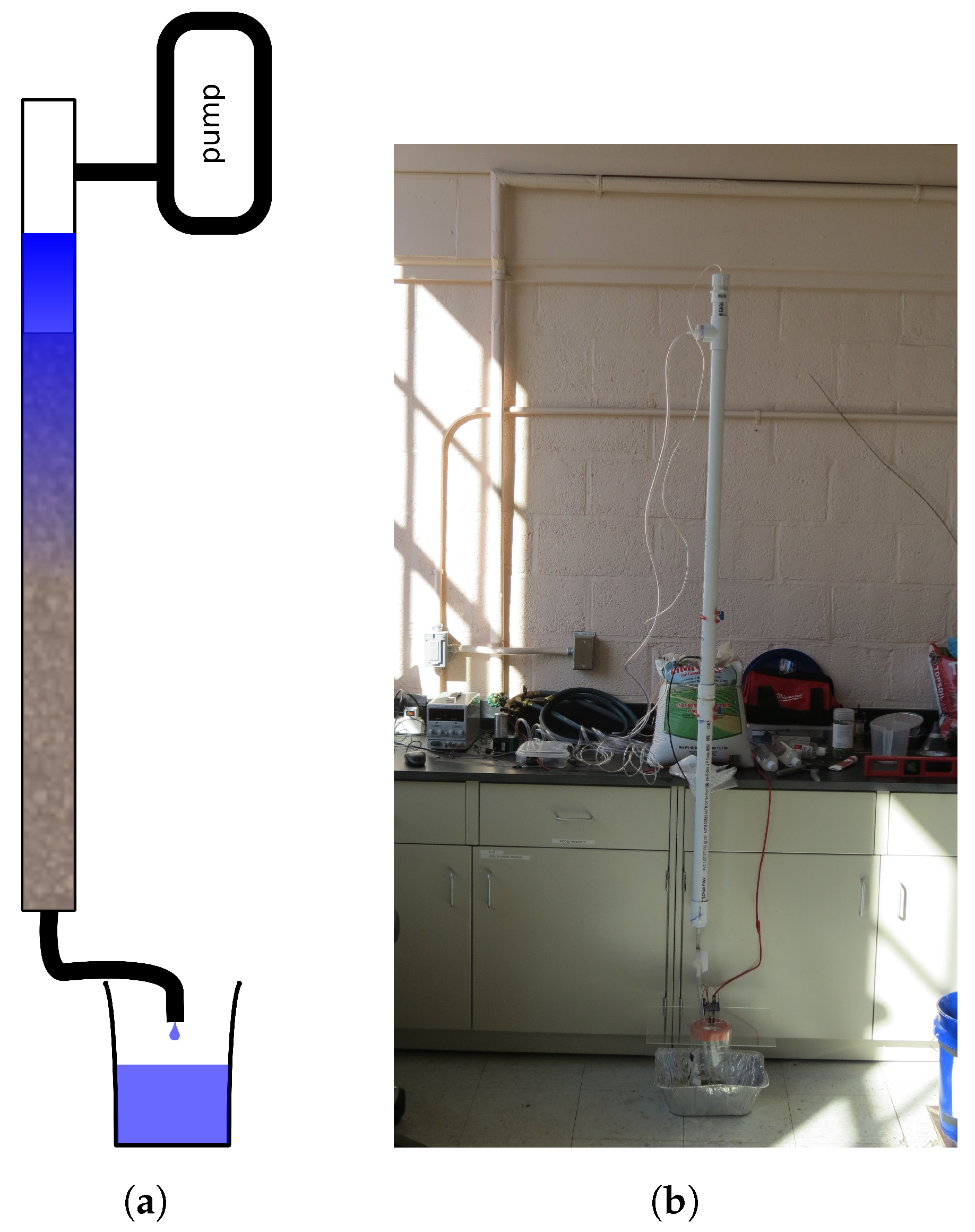
The previous section introduced a complete inductive algorithm for identifying novel variables that expand the degrees of freedom in terms of which we describe the world. What remains is to demonstrate the scheme for parameter conversion—the induction of a new variable—in action. To that end, I carried out a number of experiments with the potential to reveal a rich set of new variables. These experiments concern the movement of water through soil. As elemental as that may sound, in both senses of the word, predicting the manner in which water moves through various substrates is actually a complex, multi-scale problem so far as modern physics is concerned. Most of the models used to actually predict, say, the flow of groundwater are “empirical” in the sense of constituting regressions from data rather than derivations from first principles. But the established models of water movement through soils do not concern us. The point is to approach such systems with a naive gaze and to see how novel variables are generated from a given base set. In this case, we begin with only a single variable, volume, observed through time. More precisely, we have at our disposal the volume of water that has passed vertically through a column of soil observed at regular time intervals.
There are additional details necessary to characterize this volume variable. A cartoon sketch of the experimental apparatus can be found in Figure 3a. The heart of the thing is a vertical tube (the test section) that is roughly 2 m long with a 3.18 cm inner diameter. The lower portion of the test section is filled with a sample of soil (200 mL) followed by a volume of water (1200 mL). In each experiment, this water is allowed to pass downward through the soil sample and out through a 0.95 cm diameter hole. From there, expelled water passes through a short flexible tube into a collection beaker. The volume in the collection beaker is monitored by an automated system with a sampling frequency of 10 Hz.14
The apparatus is also fitted with a system for pressurizing the test section to a constant pressure up to a maximum of around 1200 hPa (1.2 atm). I have not, however, included pressure among our stock of given variables. As we’ll see, something equivalent to the pressure head on the column of water emerges as a novel variable from the volume data.
When the test section is filled with sand, typical timeseries for the volume of water flowing through the sample look like the pair depicted in Figure 4a. In the figure, the filled tan circles are actual measured volumes (with some obvious noise), while the black lines show the data smoothed with a rolling average. While it is a little obscure for the sand data (though obvious for the topsoil data in Figure 4b) there is significant variation in behavior apparent for one and the same sample of material. Importantly, these differences are repeatable and consistent—we get the same curve (within sampling error, of course) when we start with fresh, dry sand and likewise for sand that has had water run through it until it passes all 1200 mL. Furthermore, this variation occurs within a single dynamical kind—the sort of natural class for which Rozeboom’s parameter conversion inference is warranted. How do we know this? The dynamical symmetries implicit in both timeseries for sand are plotted in tan in Figure 4c. Even casual inspection indicates that the roughly linear relationship between transformed and untransformed curves is the same for both time series. In other words, all the tan points lie on the same curve, which means that despite their superficial differences in behavior, each experiment with sand is an instance of the same dynamical kind.15 This variation is robustly repeatable, and corresponds to a simple context: the retention of water. All of the prerequisites having been established we can—or, indeed, are compelled—to recognize a new variable, one that varies with the amount of water retained by the sample of sand.
Quantifying this new variable is another matter. For starters, since the empirical feature that distinguishes the context for each distinct volumetric curve is the volume of water retained in the test section indefinitely, we may as well use that value as the value of our new variable. Calling the new variable “wettability”16, the wettability of sand in the curves shown is 0 mL for the sand of the upper curve and 100 mL for the lower. So far then our procedure has, for experiments with sand alone, yielded a new variable describing complex granular materials like sand.
Once we begin varying the composition of the soil in the test section, a richer vocabulary of variables (or a richer ontology depending on one’s stance) imposes itself. Figure 4b shows a pair of runs of the experiment with 200 mL of topsoil in lieu of sand. The first thing to notice is that, like sand, there is variation across iterations of the experiment but, as the overlapping green symmetries in Figure 4c demonstrate, each iteration is an instance of the same dynamical kind. These variations are again indicative of the influence of another variable, which we can recognize as the wettability variable introduced above. In this case, the values are 100 mL for the upper curve and 0 mL for the lower. But there is more. We can now fix the value of wettability as part of our experimental context and note that the volume-time behavior varies between sand and topsoil. Note that the time axis for the topsoil plots in (b), is the same as those for sand in (a). The upper curve in (b) and the lower in (a) both have a wettability of 100 mL. But they clearly differ; the water flows through the topsoil much faster than the sand. However, as Figure 4c demonstrates, sand and topsoil exhibit the same dynamical symmetry (the green curves in (c) rest on top of the tan). This is therefore another variation—variation across soils—that warrants inference of an additional variable I call intrinsic resistance. In the experiments reported, only a discrete handful of soil types were available. Consequently, there is no need to assume that our new variable must be represented by the reals as opposed to a discrete set of qualitative labels. However, it is convenient to identify values of that variable with the time taken to yield half the added water (i.e., 600 mL). So we have for sand, at a wettability of 0 mL, an intrinsic resistance of roughly 267 s and for topsoil (also at a wettability of 0 mL) an intrinsic resistance of 90 s.
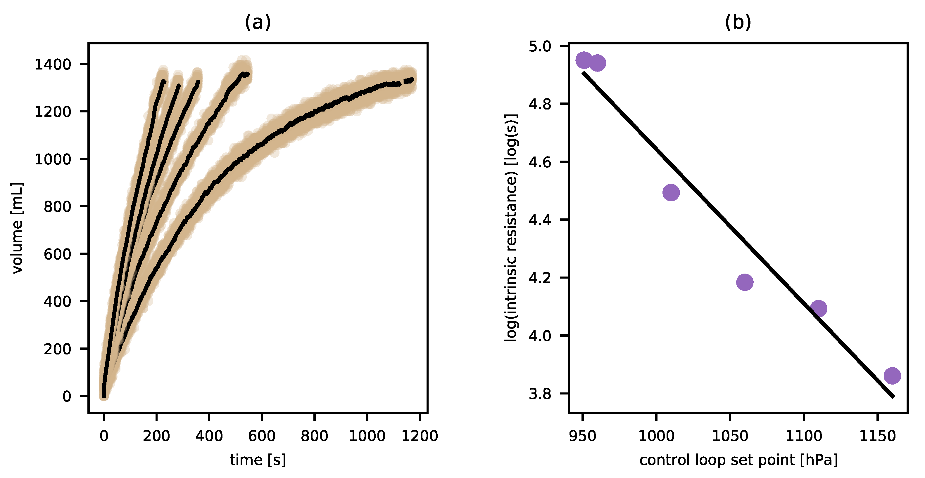
Finally, having identified wettability and intrinsic resistance, we can fix their values for a given test substance and seek for remaining variation. This time, the variable context is provided by the set-point of the pump feedback loop which corresponds roughly to the pump duty cycle.17 With a sample of sand in the test chamber brought to a wettability of 0 mL, samples of water were passed through while the pump duty cycle was held at increasingly high values. The resulting timeseries of expelled volume are shown in Figure 5a. As in our other experiments, these curves all exhibit the identical dynamical symmetry18, and so each system (each test with the pump at a different duty cycle) belongs to the same dynamical kind. But each curve is clearly distinct. In particular, the intrinsic resistance is different for each.19 We are thus induced to introduce a final variable, which we may as well call “pressure head”. We can assign the value of the control loop setting as the value of this pressure head. Since the sensor used in the control loop was calibrated in hectopascals, I’ll use those units for pressure head as well. But note that we are a long way from introducing a variable equivalent to pressure in general. In particular, our pressure head variable is introduced with no known relation to forces, relation to volume, or most of the other features associated with the existing concept of pressure in physics. While I believe there is an equally perspicuous logic that guides the generalization and abstraction process that takes one from a particular variable like our pressure head (or the gas-tube temperature discussed above) to an abstract variable like “temperature” or “pressure” tout court, this would take another essay to explicate.
For now, it suffices to examine the particular pressure head variable pertaining to this particular experimental arrangement. There was no a priori guarantee that water moving through sand under increasing pressure would provide instances all of the same dynamical kind. Perhaps under pressure, the whole thing might have acted differently; the volume expelled as a function of time might have taken on a more linear functional form, or perhaps something hyper-exponential. As with wettability and intrinsic resistance, it is not trivial that such a variable should exist. Furthermore, there are significant relations among our introduced variables. In other words, the introduced variables themselves participate in law-like regularities. For example, Figure 5b shows that the intrinsic resistance is exponentially related to the pressure head.
It is also the case that the law-like relations among our introduced variables may vary from one system to another. In other words, there may be distinct dynamical kinds—distinct types of causal system—involving water flow through a substrate that are distinguished by the differing relations among introduced variables. In fact, the data presented here already shows this must be the case. Suppose we consider the dynamics of drying. That is, imagine we take a sample of either sand or topsoil, fix its initial intrinsic resistance at a desired value (by changing its wettability), and observer how it’s intrinsic resistance changes over time as the sample is dried out at some fixed temperature. Like water flow through a substrate, drying is a complex process involving fluid flow, molecular adhesion, and thermodynamic interactions. The data described above already tell us that as the amount of water in sand diminishes (and so its wettability increases), the intrinsic resistance increases. However, as the amount of water in topsoil diminishes, its intrinsic resistance decreases. It is thus not possible for them to share a dynamical symmetry. For one and the same amount of drying, the dynamical symmetry mapping curves of intrinsic resistance versus drying time for sand must be an increasing function of drying time, while that for topsoil must be decreasing. We have discovered that sand and topsoil are in some ways very different causal systems. More to the point, we have found that in every sense, our algorithmically derived novel variables introduced by way of parameter conversion can play the same roles in inference (and presumably in control) as the single classical variable of volume with which we began.
6. Variables, Induction, and Measurement
I have implied from the outset that the corpus of philosophical and mathematical work falling under the rubric of measurement theory does not resolve the riddles motivating this paper: what is a variable; how do we come by novel variables; and what justifies their introduction? However, measurement theory is not irrelevant to these questions either. It may help to illuminate both the problems that concern us here and the problems central to measurement theory if we examine their overlap, at least in brief.
As understood by measurement theory, measurement involves (in whole or in part) the assignment of numbers (generally the reals) to physical qualities. Campbell [31] (p. 267), for instance, says that “measurement is the process of assigning numbers to represent qualities.” But not just any assignment will do. There must be some sort of consonance between the structure of the class of qualities being measured and the structure of numbers themselves. As Suppes and Zinnes [32] (Section 2, p. 7).20
Put it, the first fundamental problem of measurement is the “justification of the assignment of numbers to objects or phenomena.” Recall that a variable is an equivalence class of triplets, where P is a partition of physical states (the same partition for all members of the equivalence class) while each R is a class of representations (e.g., the real numbers) and f is a map from P to R. Many choices of R have innate structure. For example, using numbers as representations of physical qualities—rather than merely the numerals as an otherwise meaningless set of labels—means that there are many relations among the representational vehicles. Some numbers are larger than others, divisible by others, etc. There are intervals on the real numbers with natural measures that allow their comparison, and so on. Insofar as scientists wish to reason backward from such relations to relations among the physical somethings in P, we must ensure that there is enough structure in P in the first place to answer to these relations among numbers, and must choose a mapping f that ensures that structure in P is mirrored in R and not vice versa. The founders of measurement theory took it as their central task to “[c]haracterize the formal properties of the empirical operations and relations used in the procedure [of measurement] and show that they are isomorphic to appropriately chosen numerical operations and relations” [32] (Section 2.1, p. 9). To put it in my terms then, the question at the center of measurement theory is the following: for a given P, what choices of R and f are permissible or optimal given some normative assumptions about the nature and uses of such representations?
An answer to this question says something about the aptness of various representational schemes. It tells us when the real numbers, for instance, make sense to use as R so as, to quote Campbell again, “to enable the powerful weapon of mathematical analysis to be applied to the subject matter of science” [31] (pp. 267–268). It puts constraints on f and R given a particular P, but it does not tell us much about about what classes of qualities to consider in the first place. What it does say is problematic. As Aldo Frigerio, Alessandro Giordano, and Luca Mari [33] have pointed out, the constraints placed on empirical relational structures—i.e., the class P and the empirical relations that obtain among its members—by the representational theory of measurement (the dominant school of measurement theory) are both too strong and too weak. They are too strong in that the sort of structures they demand in order for a variable to be measurable with either interval or ratio scales [34], are unlikely to be realized by any empirical system as they require sequences of arbitrarily small quantities. They are too weak in that saying an empirical relational structure can be represented by a relational structure on the real numbers is equivalent to saying that the cardinality of states in the empirical structure is no greater than that of the reals. Even if it did place stronger constraints on P, measurement theory (or at least the representational theory of measurement) still wouldn’t tell us anything about how to determine which member of P we’re looking at so as to properly apply f. In other words, the grand irony of measurement theory is that it has little to say about what it is that gets measured and what counts as an act of measurement. This is not a criticism of measurement theory, merely the observation that it has directed itself to questions distinct from those that concern us here.
There is, however, an interesting connection. Even in its most general form, the fundamental question of measurement theory presumes that R is supposed to capture not just P in some convenient form, but something of the empirical structure of P.21 The condition (C2) for parameter conversion, which ensures that a variant relation is not an accident of noise or data clustering, requires identifiable conditions for determining the presence of each variant. In other words, and are related by f in one context and in another, where each context is a set of sufficient, qualitative or quantitatively characterized conditions. In the example of Section 4, the material composition of the sphere (lead vs. aluminum) provided such a set of contexts. Insofar as we are able to bring about these contexts at will and are aware of a procedure for doing so, then we have a set of operations of the sort with which measurement theory is concerned. In other words, the satisfaction of condition (C2) essentially guarantees a set of empirical relations among elements of P of the sort that measurement theory asserts must be captured by corresponding relations among elements of R. Thus, the account of variable genesis defended here ensures that the values of a variable are such that from the inception of the variable, we are aware of structure worth representing. However, it is perhaps more important that parameter conversion provides an effective recipe for identifying new measurable properties in the first place, another aspect of measurement about which measurement theory is silent. Furthermore, we can start to say something about which acts counts as acts of measurement (or what processes are measurement processes): an act of measurement is the ascertainment of the value of a variable. Since the latter is defined without explicit or implicit reference to measurement, there is no vicious circle here, only a place to begin building necessary and sufficient conditions for measurement. It is clear then that a theory of variables has something useful to say about the foundations of measurement. What of the other way around?
One way measurement theory might contribute to the theory of variables is by terminating a regress. There must be a basic set of variables not induced by parameter conversion; it can’t be turtles all the way down. I hold the view that most variables are, if not explicitly constructed by way of parameter conversion, ultimately attained through a process that imitates it or can be rationally reconstructed as such. But it cannot be that all are obtained this way. There must be some raw materials from which to begin this complex bootstrapping process of building out a scientific ontology. So what are these basic or atomic variables? Perhaps a theory of “fundamental measurement” helps resolve this mystery. Campbell [31] and like-minded measurement theorists understand a fundamental (as opposed to derived) measurement to be one which does not depend upon the measurement of any other properties. For this to be possible, it is claimed, there must be an empirical means of assessing relations of equality and comparative magnitude for the property in question, as well as a procedure for combining instances of the property in a manner isomorphic to addition. While I do not think we should insist that the values of every quantitative variable possess arithmetic structure under known empirical manipulations, it is nonetheless necessary that there be fundamental variables that do not depend on others for their definition. Furthermore, the set of values for each of these fundamental variables must be rich enough to sustain parameter conversion. That is, there must be enough values that meaningful patterns of change through time and variations of these patterns can be discerned. So perhaps the putative fundamental measurements are indicative of the requisite atomic variables.
More modestly, measurement theory is important for the use to which I’ve put it above. Once a variable has been identified, we naturally want to choose an R and f such that the tools of mathematical analysis can be applied. As I said, each variable is born with at least some empirical structure on its values, and measurement theory by way of its rich set of representation theorems can tell us what sort of scale (what sort of R and f) is suitable for capturing that structure while giving us the greatest analytic power. These are merely coarse suggestions, and shouldn’t be mistaken for a finished proposal. The point is that although a theory of measurement does not resolve all questions about the nature and origin of variables, accounts of both are mutually informative and restricting.
What then of induction? To this point, I have endeavored to demonstrate how many or most variables are introduced (or can be rationally reconstructed as having been introduced) by way of an inductive procedure. But of course, variables feature in this procedure as well as all of the central inductive inferences of science. It remains then to remark on the ways in which the inductive provenance of a variable bears on its utility in further inductions.
In one of the few existing works to explicitly address norms of variable identification, Woodward [36] (p. 1054) says we should “[c]hoose variables that are well-defined targets for (single) interventions in the sense that…there is a clear answer to the question of what would happen if they were to be manipulated or intervened on”, and “that have unambiguous effects on other variables of interest under manipulation”. Let us suppose that interventions are well-defined if and only if it is possible to clearly describe a circumscribed set of changes in the world that would necessarily be brought about by such an intervention. Let us further stipulate that the effects on a variable of an intervention on a variable are unambiguous if and only if an intervention that brings to the value x never decreases the probability that on one occasion while increasing it on another. That is, setting uniquely determines a probability that , all else being equal (i.e., when there are no other causes of that change value). If every variable used to induce a novel variable through parameter conversion satisfies these two conditions, then so too does ; well-posed variables beget well-posed variables. Consider a pair of variables and where . Suppose that interventions on either of these are well-posed in that there is a clear answer to what must be true of the world when , and similarly for . Furthermore, there is a function f such that ; ’s effect on is unambiguous. If we are led to introduce a new variable by parameter conversion, then we know what must change in the world when is intervened upon: changing just means changing the relation between and . Furthermore, the effects of on are unambiguous. This is because we can write the values of as a function of both and ; for every pair of values x and z there is exactly one value of .
Of course, there is no guarantee that is well-posed as a cause of some other variable not considered in the introduction of . It’s always possible that nature will force us to refine our variable set still further once additional effects are considered. This is exactly what happened above with wettability when we were forced to recognize intrinsic resistance. This is also true, incidentally, of the macrovariables described in Section 4 and Appendix A. They are well posed by construction with respect to the set of effect variables with which one begins. However, they may cease to be well-posed when new effects are considered. This should be neither surprising nor a source of skeptical alarm. There is an obvious method for detecting and correcting this occurrence: if a particular intervention on a variable reliably gives one effect in one set of circumstances and a different effect in another, then introduce a new variable the values of which change between those circumstances. This is just parameter conversion!
With respect to intervention, Woodward [36] (p. 1054) also suggests that we choose “variables that are defined in such a way that we can in principle manipulate them to any of their possible values independently of the values taken by other variables”. This might appear to pose a problem for given its essential connection to both and . However, the values of correspond to (though need not be viewed as identical with) the relation between and , not any particular values of those variables. Furthermore, condition (C2) for parameter conversion requires a reliable (invariant in Woodward’s terminology) connection between identifiable conditions and the presence of a particular – relationship. It is thus possible to intervene on all three variables independently, given that it’s possible to intervene on and independently. That is, we simply intervene on the conditions necessary for a particular – relation, and this can be done independent of the value of either or .
The upshot is that variables induced through parameter conversion satisfy a gamut of norms on the nature of variables for use in inductive inference, and it is the provenance of these variables as products of a distinct inductive procedure that guarantee they possess these properties.
7. Conclusions
Variables are the warp and woof of scientific inference, and yet their nature has remained largely unexamined. I have argued that we should view each variable as an equivalence class of triplets, each consisting of a partition, P, of the physical states of the system to which the variable pertains, a set R of representations, and a mapping f from P to R. While P is fixed for a system and the same in every triplet of the equivalence class, R and f can vary so long as each mapping preserves relevant structure on P. This is a modest modification of the accounts developed by Karl Menger and W. W. Rozeboom in the 1950’s and 60’s. Whether or not the details of my proposal are convincing, the salient kernel of clarity is that variables are a coordination between physical somethings and representational somethings.
More important is the way in which variables relate to inductive inference. On the one hand, there is the uncontroversial fact that an appropriate set of variables is necessary for successful induction. In fact, one of the hyperbolic objections to the automated discovery programs produced by Herbert Simon’s group in the 1980’s was that the program creators had provided the variables in terms of which, say, Kepler’s Third Law of Motion would be especially perspicuous, and that this constituted all of the creative effort of discovery; once you’ve got sun-centered coordinates, the rest is trivial curve fitting. Langley et al. [13] rightfully rejected this extreme view, but the point remains: working with some variables makes regularities discoverable, while others make discovery hopeless. Lately, there has been increasing interest in the epistemic problem of exactly how variables can support or undermine successful inductive inference. Increasingly, philosophers are recognizing that there is something normative and productive to say about this problem.
What the arguments and demonstrations above are meant to establish is that the converse is also true: the identification of most variables can and should be viewed as the end product of a particular sort of inductive inference. From a stock of well-posed variables, we identify new variables by way of parameter conversion: variation in a law-like regularity within a natural kind implies an unrecognized variable responsible for that variation. While this template is W. W. Rozeboom’s, he left unresolved the relevant sort of natural kind and how one might detect its boundaries empirically. In the foregoing, I have suggested that dynamical kinds complete this template. Dynamical kinds are equivalence classes of dynamical causal systems that share enough causal structure to sustain useful generalizations across the class. More to the point, variation within that class in a relation between two variables suggests the causal role of a third. Importantly, one can determine whether or not two systems belong to the same dynamical kind from experimental data without first learning the detailed causal structure of either. Thus, with the choice of dynamical kinds, I have presented a full algorithm for variable identification: when the robust association among variables varies from one context to another for systems within the same dynamical kind, introduce a new variable to account for this variation.
In Section 5, I demonstrated the efficacy of this algorithm in studies with water passing through granular media. Beginning with a single volume variable, those experiments led to the inductive identification of wettability, intrinsic resistance, and pressure head. The latter two were guided in part by values of the previously introduced wettability variable. Furthermore, the introduced variables supported law-like generalizations describing the causal relations among them (e.g., internal resistance is exponentially related to pressure head). That they should be useful for doing so ought not to be surprising—I argued in Section 6 that well-posed variables beget well-posed variables with respect to a number of norms governing variable choice for inductive inference. Furthermore, the experimental results indicated a difference in dynamical kind between drying topsoil and drying sand—our novel variables have led us to new classes for which to carry out additional parameter conversion inferences.
Aside from a demonstration of the aptness of Rozeboom’s parameter conversion, the experiments reported here—and the algorithmic introduction of novel variables they support—provide as clear a counterexample as one could imagine to the thesis that a logic of discovery is impossible. But that does not settle the status of the induced variables. That is, the ontological implications of an induced variable remain undetermined. One could, as Rozeboom does, see the new variables as indicative of hidden or unobserved properties in the world. Alternatively, one may take a strongly empiricist stance and view the new variables as compact summaries of relationships among the variables from which they were derived. I do not pretend to settle this issue here. Nor have I attempted to grapple with the potential arbitrariness of the set of induced variables with which the scientist ends up. It would seem that the choice of initial variables determines which new variables will be discovered. Furthermore, there may be a history dependence—which variations in law-like relations are considered first may change the set of variables ultimately induced. Whether and under what conditions this is so remain to be examined, as do the ontological implications of this sort of path dependence.
These open avenues for further inquiry will, I hope, spur the reader to a closer examination of the nature of variables and the reciprocal relationship between variables and induction. I do not claim (nor do I think) that scientists always proceed by parameter conversion. But this simple algorithm allows for the rational reconstruction of an enormous range of scientific innovations, and opens up the possibility of inferences equally sound yet unconceived. The logic of discovery remains fertile ground for philosophers of science and practitioners of artificial intelligence alike.
Funding
This research was funded by the National Science Foundation (Grant No. 1454190).
Data Availability Statement
All data generated in the reported experiments are openly available from the Virginia Tech Data Repository at https://doi.org/10.7294/17153288. The particular files used to generate the results reported in Figure 4 in the text have the following names: sand_900.0_10.0_21.5_Mon_Oct_28_13:37:00_2019, sand_900.0_10.0_22.125_Mon_Oct_28_14:06:53_ 2019, topsoil_900.0_10.0_23.125_Tue_Oct_29_13:15:30_2019, topsoil_900.0_10.0_24.187_Tue_Oct_29_ 14:50:16_2019. The files containing data used in the pressure studies reported in Figure 5 include the following: sand_900.0_10.0_22.562_ Mon_Nov__4_13:07:53_2019, sand_960.0_10.0_24.375_Mon _Nov__4_13:37:13_2019, sand_1010.0_10.0_26.312_Mon_Nov__4_14:06:45_2019, sand_1060.0_10.0_27. 375_Mon_Nov__4_14:28:19_2019, sand_1110.0_10.0_27.25_Mon_Nov__4_14:43:04_2019, sand_1160.0_ 10.0_26.937_Mon_Nov__4_14:58:00_2019.
Acknowledgments
I am grateful to Parisa Farhi for suggesting the use of parsley in the experimental apparatus when no other available commercial or industrial materials seemed up to the task.
Conflicts of Interest
The authors declare no conflict of interest. The funders had no role in the design of the study; in the collection, analyses, or interpretation of data; in the writing of the manuscript, or in the decision to publish the results.
Appendix A. Inductive Genesis of Dimension-Reducing Scientific Variables
There are well-established methods for generating novel variables that reduce the apparent degrees of freedom in terms of which the world is described. In machine learning, such methods fall under the rubric of “dimensionality reduction” and include techniques like principal component analysis and manifold learning. While appropriate (with caveats) for prediction based on passive observation, these methods neither aim nor succeed at capturing the sort of causal information for which scientific theories typically strive. While, for instance, it may be that the first few principal components, of a large set of variables are sufficient to predict the values of a target variable, , this tells us nothing about whether the are causes of . In fact, given the way principal components are constructed, it is ambiguous what it would mean to even manipulate the value of each to see if this has an effect on . This is because principal components are linear combinations of variables. For instance, if we begin with two variables and , the first principal component will have values given by for some real and . But then an intervention on is ambiguous. Changing the value of could mean changing , , or both. If and have different effects on some other variable, then intervening on will exhibit contradictory effects on that variable. Furthermore, even if some or all of the are causes of , they may be muddled reflections of more efficacious causes. Whatever their predictive acumen, the failure of such variables to give us control or capture the counterfactual structure of the world makes them poor candidates for respectable scientific concepts.
From the standpoint of scientific variables, what we want of an algorithmic approach to generating new variables of this sort is the ability to identify the lowest-dimensional set of causes (and perhaps the lowest-dimensional description of the effects) that exists for a phenomenon of interest. In other words, given some large stock of variables, some of which describe the effects of interest and some of which are putative causes, we need a method for constructing an alternate set of variables of equal or lesser dimension that captures all and only the information about how states of the one alter the states of the other. Returning to my piston example, we want an algorithm to tell us that a single new variable—the average pressure in the combustion chamber—is all that’s relevant for determining the force on the push rod to which the piston is connected. “Determining” here is meant in the causal sense that if we wish to cause a particular force or if we wish to predict what would be the force under a different set of pressures, then this is what is matters—the average pressure says it all.
This is precisely what the work of Chalupka, Eberhardt, and Perona [8,9] provides: an algorithm for identifying the “macrocauses” (and macroeffects) implicit in a large set of microvariables. More specifically, given a (typically very large) collection of cause variables and a similar set of effect variables, they first partition the joint states of these microvariables into equivalence classes with respect to the probability of the effect variable(s) conditional on the joint state. This partitioning is called the observational partition. It is then possible to efficiently use experiments to partition the joint states of the microvariables into equivalence classes with respect to the probability of the effect given an intervention that puts the system into a particular microstate. The reason we know this can be done efficiently—typically with vastly fewer manipulations than would have to be carried out if we had to consider all combinations of the microvariables rather than just the cells of the observation partition—is the “fundamental causal coarsening theorem” [8]. This theorem tells us that the causal partition we seek is almost always a coarsening of the observation partition. The result of these efforts is a one-dimensional macrovariable, the values of which correspond to cells of the causal partition and preserve all of the causal information that was present in the microvariable description (relative to the target effect) and nothing more.
Whether one is inclined to grant the variables so discovered or produced the status of a genuine property in the world ultimately rests on commitments beyond the scope of this essay to examine. But if one is looking for “joints” in nature, the causal hinges as reflected in the causal macrovariables seem like prime candidates. The fact that manipulation of macrovariables defined in this way is well-posed and that manipulating a macrovariable lets us manipulate its effect(s) endows those macrovariables with the sort of qualities that provoke reification. Such qualities are, for instance, why we take a macrovariable like “atmospheric pressure” seriously as a feature of the world.
This doesn’t quite settle all issues surrounding the definition or use of composite variables. For instance, we may not know which of many microvariables are causes, and which are effects. We may not even have access to the relevant microvariables in the first place [37]. Regardless of how we answer these remaining questions, it is clear that such variables can and should be viewed as the outcome of an inductive procedure.
| 1 | To be clear, Rozeboom does not explicitly identify these problems or indicate that the way in which his proposal differs from Menger’s is intended to address such difficulties. |
| 2 | Menger [2] (p. 464) says the same thing more explicitly: “Thus extramathematical features (such as “denomination” and “dimension”) that are often attributed to the values of [gas pressure in atmospheres] are, as it were, absorbed in the definitions of these fluents”. |
| 3 | We might just as well take the value of a variable to be an equivalence class, specifically the union of the image of under each in each corresponding . In that case, not even the value of the variable changes when we change units, only the expression of the value. |
| 4 | For completeness, it is also possible to induce a novel set of variables that leaves unchanged the degrees of freedom. In such a case, the novelty would consist in drawing cross-cutting distinctions about states of the world. Methodologically, this possibility is probably best construed as a special case of dimension-reducing induction, but investigating this interesting class of possibilities would take us too far astray from our present concerns. |
| 5 | I have elided much of the logical subtlety of Rozeboom’s technical presentation. In particular, I have ignored the successively higher logical types of introduced variables in the Russellian sense of a type-hierarchy of particulars, classes, classes of classes, etc. Rather, I treat all variables as of a kind, and I express relations in terms of functions. While doing so comes at the cost of some of Rozeboom’s precision, it avoids the notational burden, and captures what I take to be both salient and correct in his proposal. |
| 6 | So far as I can tell, Langley et al. never acknowledged the work of Rozeboom. It’s puzzling that they should be unaware of it given the overlap in publishing venues between Simon and Rozeboom, but that appears to be the case. |
| 7 | Not all causal variables are equally apt for control and prediction; those epistemic goals can come apart. See [14]. |
| 8 | See [16] for an innovative discussion of the epistemic problems posed by the failure of equilibration and intervention to commute when the time scales for these processes are comparable. |
| 9 | I mean this loosely, not in the strict sense of an algebra over a field. Symmetries under composition are unlikely to constitute a group or even a monoid in the precise mathematical sense. There may be no inverse for some interventions—some symmetry transformations—and some compositions of symmetries may exceed the limits of “invariance” for the system in the sense that they may induce variable values that break the original causal relation, like overstretching a spring. |
| 10 | See [24] for a defense of dynamical kinds as natural kinds. |
| 11 | Likely with a vanishingly small set of exceptions. |
| 12 | This is true if we take the points in order. If we ignore order, then for any two points a and b, there is a unique pair of trajectories A and B that pass through them, respectively. The function that maps A to B will, in general, be distinct from that mapping B to A, so there are two dynamical symmetries. |
| 13 | Gas thermometer temperature is not temperature simpliciter, but that’s a topic for another time. |
| 14 | More accurately, the level of water in the beaker is monitored with a laser ranging device, the beam of which is reflected off of buoyant opaque particles—flakes of dried parsley—that remain on the surface as the beaker fills. |
| 15 | As noted above, more sophisticated statistical procedures exist. All of the symmetries shown here were compared pairwise with the energy distance test, and found not to be significantly different. |
| 16 | I realize this is already a technical term, but the algorithm has outstripped my imagination. |
| 17 | The pump motor voltage was set by a bang-bang closed loop control system that incorporated a pressure sensor. The higher the pressure setting, the more the pump would run. However, the timing of the pump’s activation was random—depending on leakage from the test section and other factors—and the duty cycle was not directly controlled. |
| 18 | As before, this was determined using the energy distance test described in [29]. |
| 19 | There is a hysteresis effect: after being pressurized, a sample of sand has its intrinsic resistance permanently altered. |
| 20 | This early report by Suppes and Zinnes is not paginated. The page numbers given for this document are relative to the beginning and take the title page as page 1. |
| 21 | Though some have resisted this normative assumption. For an overview of the debate, see [35]. |
References
- Menger, K. What Are Variables and Constants? Science 1956, 123, 547–548. [Google Scholar] [CrossRef] [PubMed] [Green Version]
- Menger, K. An Axiomatic Theory of Functions and Fluents. In Selecta Mathematica: Volume 2; Menger, K., Schweizer, B., Sklar, A., Sigmund, K., Gruber, P., Hlawka, E., Reich, L., Schmetterer, L., Eds.; Springer: Vienna, Austria, 2003; pp. 205–224. [Google Scholar] [CrossRef]
- Menger, K. On Variables in Mathematics and in Natural Science. Br. J. Philos. Sci. 1954, 5, 134–142. [Google Scholar] [CrossRef]
- Chang, R. Chemistry, 5th ed.; McGraw-Hill, Inc.: New York, NY, USA, 1994. [Google Scholar]
- Goodman, N. Fact, Fiction and Forecast; Harvard University Press: Cambridge, MA, USA, 1955. [Google Scholar]
- Jantzen, B.C. Discovery without a ‘logic’ would be a miracle. Synthese 2016, 193, 3209–3238. [Google Scholar] [CrossRef]
- Rozeboom, W.W. Scientific Inference: The Myth and the Reality. In Science, Psychology, and Communication: Essays Honoring William Stephenson; Brown, S.R., Brenner, D.J., Eds.; Teachers College Press: Columbia, MD, USA, 1972; pp. 95–118. [Google Scholar]
- Chalupka, K.; Perona, P.; Eberhardt, F. Visual Causal Feature Learning. arXiv 2014, arXiv:1412.2309. [Google Scholar]
- Chalupka, K.; Perona, P.; Eberhardt, F. Multi-Level Cause-Effect Systems. arXiv 2015, arXiv:1512.07942. [Google Scholar]
- Rozeboom, W.W. Ontological Induction and the Logical Typology of Scientific Variables. Philos. Sci. 1961, 28, 337–377. [Google Scholar] [CrossRef]
- Brown, S.R.; Brenner, D.J. (Eds.) Science, Psychology, and Communication: Essays Honoring William Stephenson; Teachers College Press: Columbia, MD, USA, 1972. [Google Scholar]
- Bradshaw, G.L.; Langley, P.; Simon, H.A. BACON 4: The discovery of intrinsic properties. In Proceedings of the Third Biennial Conference of the Canadian Society for Computational Studies of Intelligence, Victoria, BC, Canada, 14–16 May 1980; University of Victoria: Victoria, BC, Canada, 1980. [Google Scholar]
- Langley, P.; Simon, H.A.; Bradshaw, G.; Zytkow, J.M. Scientific discovery: Computational explorations of the creative processes; MIT Press: Cambridge, MA, USA, 1987. [Google Scholar]
- Danks, D. Goal-dependence in (scientific) ontology. Synthese 2015, 192, 3601–3616. [Google Scholar] [CrossRef]
- Eberhardt, F. Introduction to the foundations of causal discovery. Int. J. Data Sci. Anal. 2017, 3, 81–91. [Google Scholar] [CrossRef] [Green Version]
- Dash, D. Restructuring dynamic causal systems in equilibrium. In Proceedings of the International Workshop on Artificial Intelligence and Statistics. PMLR, Fort Lauderdale, FL, USA, 4–7 January 2005; pp. 81–88. [Google Scholar]
- Douven, I. Abduction. In The Stanford Encyclopedia of Philosophy, Summer 2021 ed.; Zalta, E.N., Ed.; Metaphysics Research Lab, Stanford University: Stanford, CA, USA, 2021. [Google Scholar]
- Burks, A.W. Peirce’s Theory of Abduction. Philos. Sci. 1946, 13, 301–306, Publisher: The University of Chicago Press. [Google Scholar] [CrossRef] [Green Version]
- Nesher, D. Peircean Epistmology of Learning and the Function of Abduction as the Logic of Discovery. Trans. Charles S. Peirce Soc. 2001, 37, 23–57. [Google Scholar]
- Peirce, C.S. Collected Papers of Charles Sanders Peirce; Harvard University Press: Cambridge, MA, USA, 1931; Volume 5. [Google Scholar]
- Frankfurt, H.G. Peirce’s Notion of Abduction. J. Philos. 1958, 55, 593–597. [Google Scholar] [CrossRef]
- Newell, A.; Shaw, J.C.; Simon, H.A. The processes of creative thinking. In Contemporary Approaches to Creative Thinking: A Symposium Held at the University of Colorado; The Atherton Press behavioral science series; Atherton Press: New York, NY, USA, 1962; pp. 63–119. [Google Scholar] [CrossRef]
- Woodward, J. Explanation and invariance in the special sciences. Br. J. Philos. Sci. 2000, 51, 197–254. [Google Scholar] [CrossRef] [Green Version]
- Jantzen, B.C. Projection, symmetry, and natural kinds. Synthese 2014, 192, 3617–3646. [Google Scholar] [CrossRef]
- Jantzen, B.C. Dynamical Kinds and their Discovery. arXiv 2016, arXiv:1612.04933. [Google Scholar]
- Jantzen, B.C. Dynamical Symmetries and Model Validation. In Algorithms and Complexity in Mathematics, Epistemology, and Science; Fields Institute Communications; Springer: New York, NY, USA, 2019; pp. 153–176. [Google Scholar]
- Shea-Blymyer, C.; Roy, S.; Jantzen, B. A General Metric for the Similarity of Both Stochastic and Deterministic System Dynamics. Entropy 2021, 23, 1191, Number: 9 Publisher: Multidisciplinary Digital Publishing Institute. [Google Scholar] [CrossRef] [PubMed]
- Vogels, M.; Zoeckler, R.; Stasiw, D.M.; Cerny, L.C.P.F. Verhulst’s ‘Notice sur la loi que la populations suit dans son accroissement’ from correspondence mathematique et physique. Ghent, vol. X, 1838. J. Biol. Phys. 1975, 3, 183–192. [Google Scholar] [CrossRef]
- Székely, G.J.; Rizzo, M.L. Testing for equal distributions in high dimension. InterStat 2004, 5, 1249–1272, Publisher: Citeseer. [Google Scholar]
- Jantzen, B.; Roy, S.; Shea-Blymyer, C.; Hickman, M.; Mehr, J.; Gazewood, J.; Parker, J.; Karvelis, A. EUGENE (Version 0.2) [Source Code]. 2021. Available online: https://github.com/jantzen/eugene (accessed on 8 December 2021).
- Campbell, N.R. Physics: The Elements; Cambridge University Press: Cambridge, MA, USA, 1920. [Google Scholar]
- Suppes, P.; Zinnes, J. Basic Measurement Theory; Technical Report 45; Institute for Mathematical Studies in the Social Sciences, Stanford University: Stanford, CA, USA, 1962. [Google Scholar]
- Frigerio, A.; Giordani, A.; Mari, L. Outline of a general model of measurement. Synthese 2010, 175, 123–149. [Google Scholar] [CrossRef]
- Stevens, S.S. On the Theory of Scales of Measurement; Bobbs-Merrill, College Division: Indianapolis, IN, USA, 1946. [Google Scholar]
- Tal, E. Measurement in Science. In The Stanford Encyclopedia of Philosophy, Fall 2020 ed.; Zalta, E.N., Ed.; Metaphysics Research Lab, Stanford University: Stanford, CA, USA, 2020. [Google Scholar]
- Woodward, J. The problem of variable choice. Synthese 2015, 193, 1047–1072. [Google Scholar] [CrossRef]
- Casini, L.; Moneta, A.; Capasso, M. Variable Definition and Independent Components. Philos. Sci. 2021, 88, 784–795. [Google Scholar] [CrossRef]
Figure 1.
(a) Dynamical symmetries of the logistic equation, . Each curve is a trace of population over time for the same logistic model () starting from two different initial populations (5 and 35). The function that maps each point on the lower curve (such as ) to the point on the upper curve corresponding to the same elapsed time () is a dynamical symmetry of the system. In other words, this function, , is such that it does not matter whether we allow the system to evolve for some amount of time and then apply or first apply and then evolve through ; we end up at the same point on the upper curve in either case. (b) Variation within a dynamical kind. Each curve shows the evolution of a logistic system with from an initial population of 5 and a distinct value of r (between 0.1 and 11). All of these logistic systems exhibit exactly the same set of dynamical symmetries, and are thus in the same dynamical kind.
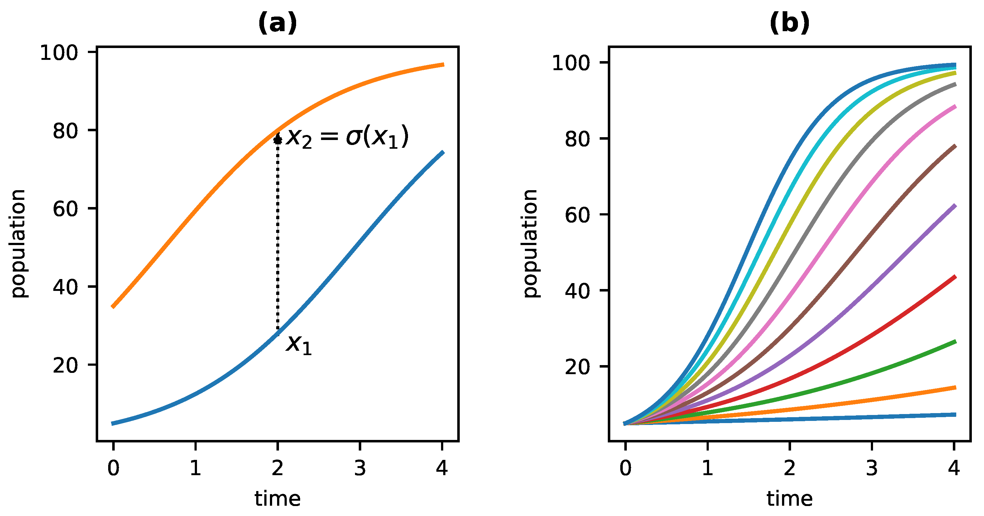
Figure 2.
A procedure for estimating dynamical symmetries implicit in a single, passively observed time series under the assumption of time-invariance. In step 1 (leftmost panel), we choose a time t midway through the time series and, in step 2, treat the data from as though it came from a fresh time series with a different initial condition. In step 3, we estimate a dynamical symmetry as before by plotting the values of one curve as a function of the contemporary point on the other.
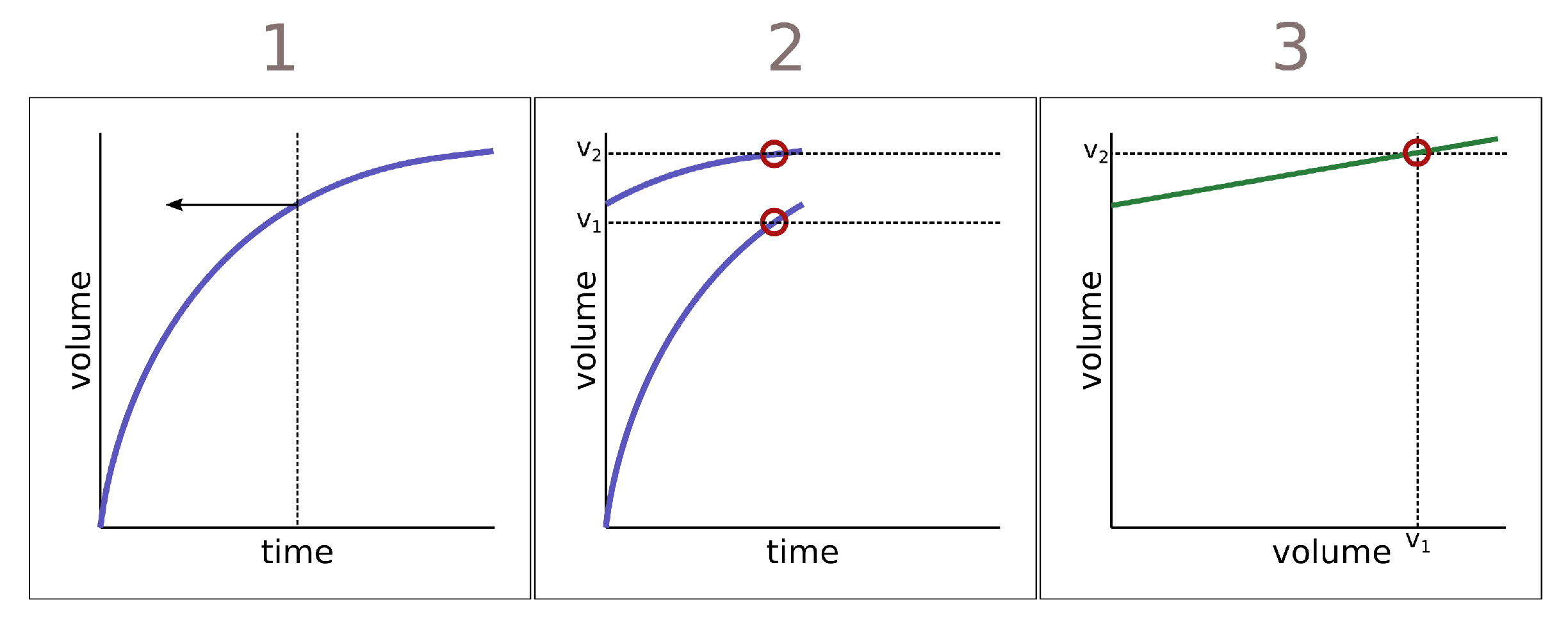
Figure 3.
The experimental apparatus used to measure the movement of water through complex granular solids. The apparatus, shown schematically in (a), consists of a vertical test section filled with sand or soil. A volume of water is added above this granular material. The chamber can be sealed and held at pressure between 1 and 1.5 atm by a pump. Water that has passed through the soil or sand is expelled through tubing at the bottom of the section and collected in a beaker where its volume is measured at 10 Hz. (b) A photo showing the actual apparatus configured as used in the reported experiments.

Figure 4.
The movement of water through sand and soil. Volume through time of a 1200 mL sample of water passing through a vertical column of (a) sand and (b) topsoil at atmospheric pressure. Each panel shows two curves representing successive experiments that differ only in how much water is already retained by the column of material (≈100 mL for the second run with either material). The implied dynamical symmetries (c) for sand (tan) and for topsoil (green) are identical.
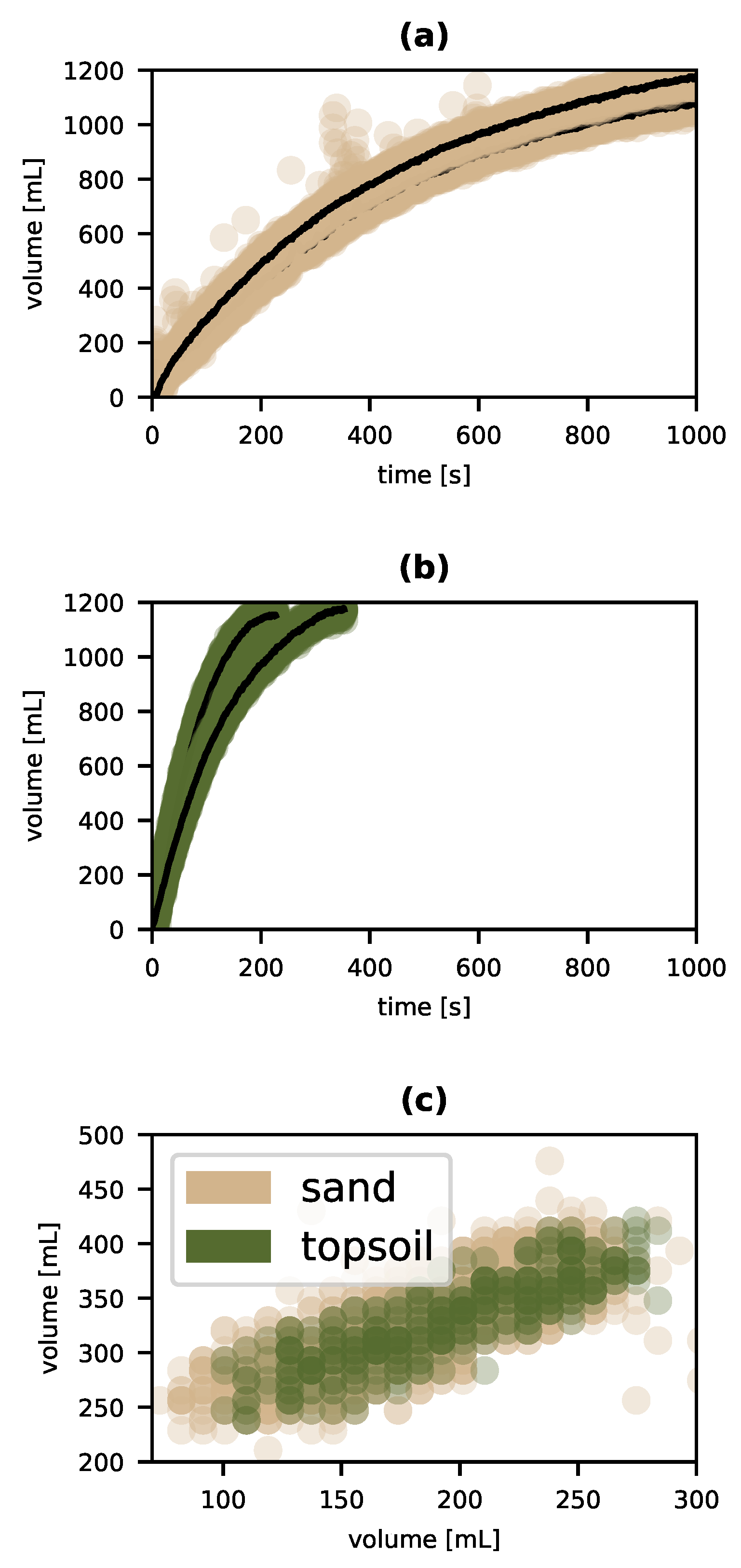
Figure 5.
Percolation of water through sand under pressure. (a) Six samples of sand were brought to a wettability of 0 mL, and 1200 mL of water were passed through the test section while the pump control loop was set at 951 hPa, 960 hPa, 1010 hPa, 1060 hPa, 1110 hPa, and 1160 hPa respectively. (b) This semi-log plot shows the exponential variation of intrinsic resistance as a function of the setting of the pump motor control loop, the values of which are equivalent to the values of the induced pressure head variable.

Publisher’s Note: MDPI stays neutral with regard to jurisdictional claims in published maps and institutional affiliations. |
© 2021 by the author. Licensee MDPI, Basel, Switzerland. This article is an open access article distributed under the terms and conditions of the Creative Commons Attribution (CC BY) license (https://creativecommons.org/licenses/by/4.0/).
Share and Cite
MDPI and ACS Style
Jantzen, B.C. Scientific Variables. Philosophies 2021, 6, 103. https://doi.org/10.3390/philosophies6040103
AMA Style
Jantzen BC. Scientific Variables. Philosophies. 2021; 6(4):103. https://doi.org/10.3390/philosophies6040103
Chicago/Turabian StyleJantzen, Benjamin C. 2021. "Scientific Variables" Philosophies 6, no. 4: 103. https://doi.org/10.3390/philosophies6040103
APA StyleJantzen, B. C. (2021). Scientific Variables. Philosophies, 6(4), 103. https://doi.org/10.3390/philosophies6040103