Effect of Hindwings on the Aerodynamics and Passive Dynamic Stability of a Hovering Hawkmoth

Abstract

Insects are able to fly stably in the complex environment of the various gusts that occur in nature. In addition, many insects suffer wing damage in their lives, but many species of insects are capable of flying without their hindwings. Here, we evaluated the effect of hindwings on aerodynamics using a Navier–Stokes-based numerical model, and then the passive dynamic stability was evaluated by coupling the equation of motion in three degrees of freedom with the aerodynamic forces estimated by the CFD solver under large and small perturbation conditions. In terms of aerodynamic effects, the presence of the hindwings slightly reduces the efficiency for lift generation but enhances the partial LEV circulation and increases the downwash around the wing root. In terms of thrust, increasing the wing area around the hindwing region increases the thrust, and the relationship is almost proportional at the cycle-averaged value. The passive dynamic stability was not clearly affected by the presence of the hindwings, but the stability was slightly improved depending on the perturbation direction. These results may be useful for the integrated design of wing geometry and flight control systems in the development of flapping-winged micro air vehicles.

1. Introduction

The application of flying robots such as drones has spread rapidly in recent years [1]. The development of processing and control technologies and the miniaturization of devices have enabled stable flight even with small airframes. However, drones still face many challenges in terms of efficiency, stability, and safety. Drones are about the same size as insects and birds, and insects and birds can be the inspiration for drones, as they have achieved high-performance flight that outperforms drones [2].

Insects generate aerodynamic forces to support their own weight and adjust their size by means of flapping wings. The aerodynamic forces to support their own weight and adjust their posture are generated by unsteady aerodynamic mechanisms such as leading-edge vortices and rotational lift [3,4,5,6]. Since the unsteady aerodynamic forces are generated by the interaction between the flapping wing and the air, the wing morphology and kinematics have a significant influence on the aerodynamic performance of a flapping wing [7]. In particular, the effect of wing morphology and kinematics on efficiency has been extensively studied experimentally and theoretically [8,9,10,11,12].

In both flying organisms and robots, flight stability is very important, along with efficiency in generating aerodynamic forces. In insects, for example, attitude stabilization is achieved by adjusting wing motion [13]. They need to control their attitude with wing motions in response to their own attitude. On the other hand, there is a reaction delay of several flapping cycles, which significantly affects their flight performance [14]. The mechanical stability of insect flight is also very important from the point of view of efficiency, etc., because in nature there are unpredictable disturbances, such as wind, and if the posture is significantly disrupted during the sensory delay, more energy will be consumed to restore the posture.

The mechanical stability of insect flight has been investigated by wind tunnel experiments and numerical simulations [15,16,17,18,19]. For example, numerical simulations have investigated the flight stability of various insects and confirmed that insects are unstable in the pitch and roll directions. Since stability and maneuverability are trade-offs, these results suggest that maneuverability is important for the insect’s habitat along with flight stability.

Thus, while the flight stability of insects has been investigated so far, the effect of wing morphology on flight stability has received little attention compared with its effect on efficiency. As the balance between stability and maneuverability is considered important in flying robots for various missions, it would be very important to derive design guidelines for flapping wings from the perspective of flight stability when creating bio-inspired flying robots.

In the present study, we focused on the effect of the presence of hindwings on flight stability, with particular emphasis on the hawkmoth as the target insect. It has been reported that lepidopterans can fly even when their hindwings are ablated [20]. This is likely due to the very small contribution of the hindwings to the generation of vertical forces, as aerodynamic forces are generated during wing flapping, especially near the wing tips. On the other hand, the effect of wing morphology on flight stability is unknown, as is the effect of hindwing ablation on flight stability. Therefore, in the present study, along with a model of the hawkmoth, a model of the hawkmoth with its hindwings removed was also created, and these models were used to investigate the effect of wing morphology, especially near the base, on the flight stability of the flapping wing by the numerical simulation. It is hoped that clarifying the effects of insect wing shape on stability will help to provide design guidelines for future wing shapes of flapping-winged micro air vehicles (FMAVs).

2. Materials and Methods

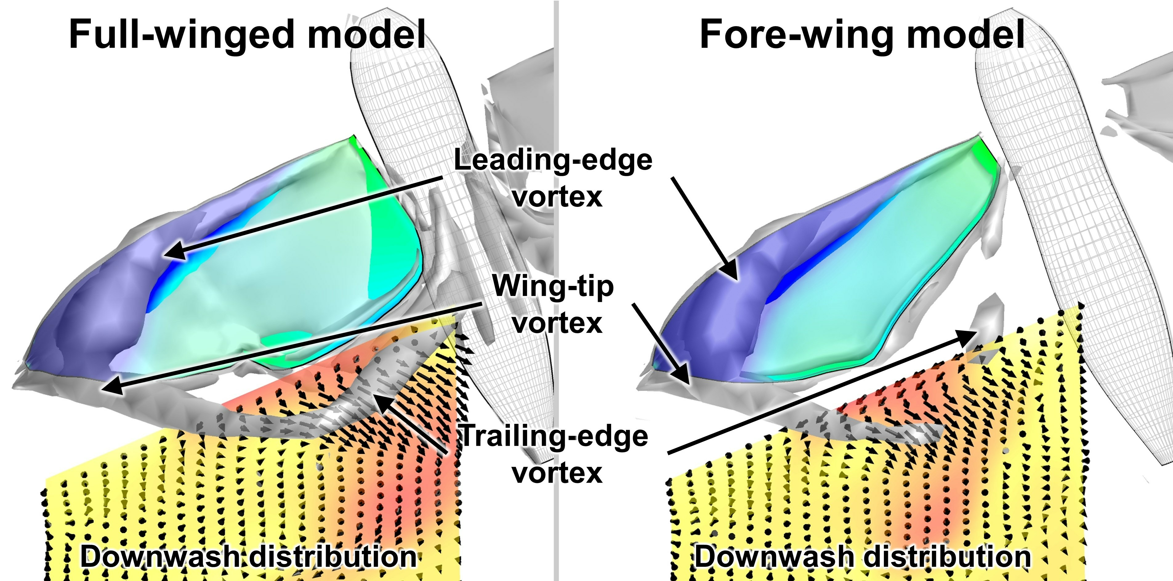
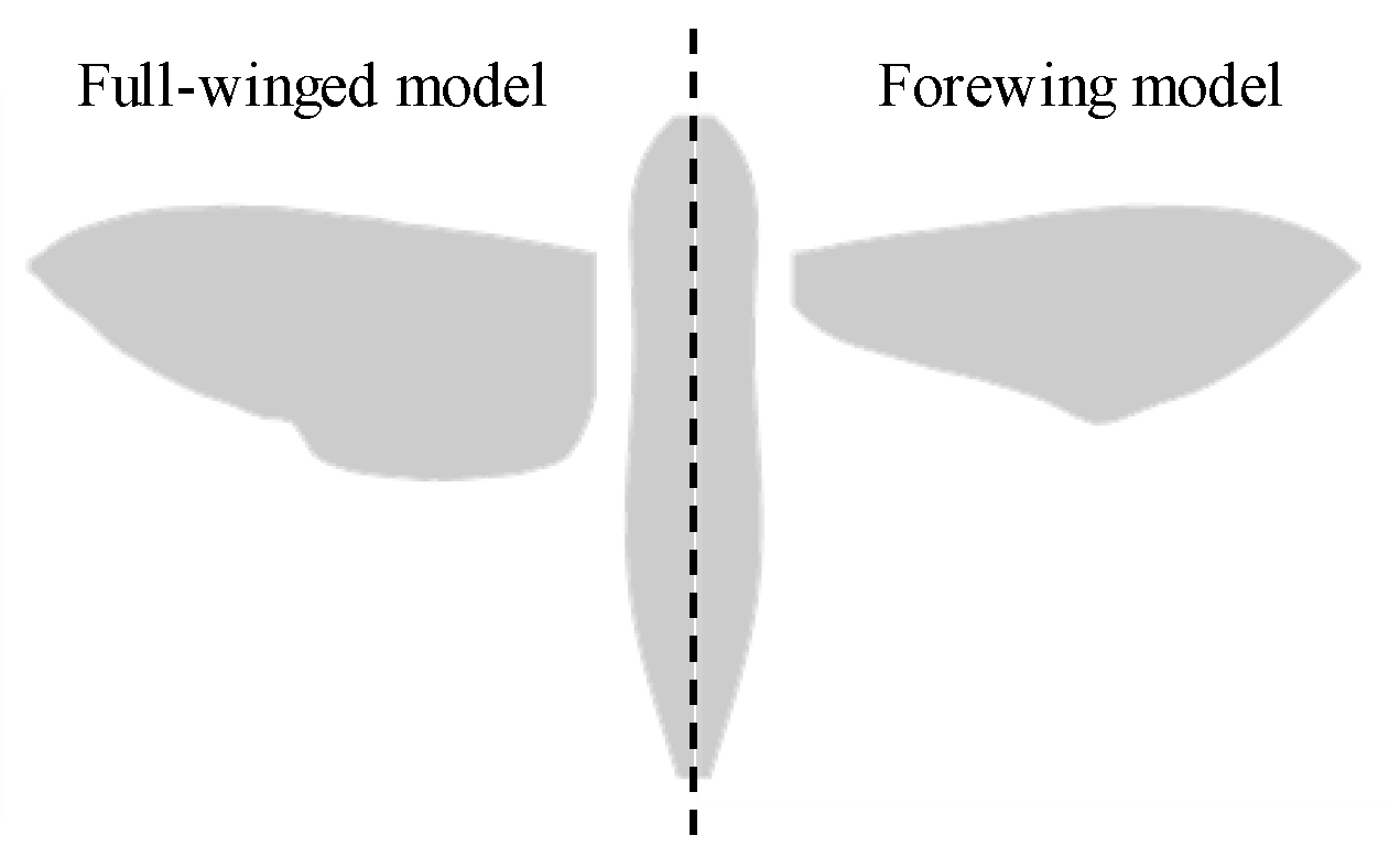
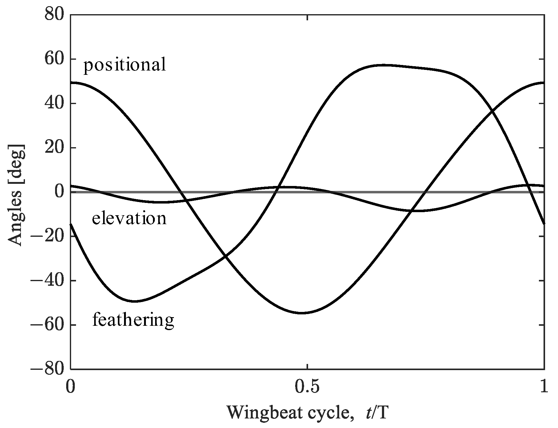
2.1. Morphological and Kinematic Model for a Hawkmoth with/without Hindwings

A morphological and kinematic model of a hovering hawkmoth, Agrius convoluvuli, was built based on an experimental observation that was filmed with five synchronized high-speed cameras (Fastcam SA-3, Photron, Tokyo, Japan), and a three-dimensional reconstruction was performed with a direct linear transformation (DLT) method via the open-source MATLAB-based application, DLTdv5 [21]. More details can be found in [22]. The reconstructed morphological model with/without hindwings is depicted in Figure 1, and the morphological parameters are summarized in

Table 1. Morphological parameters for full-winged and forewing models.

	Full-Winged Model	Forewing Model
Total mass [mg]	956	946
Wing area [mm2]	443	325
Mean chord length, Cm [mm]	12.39	9.10
Wing length, R [mm]	35.76
Stroke plane angle [deg]	36.36
Body length [mm]	41.70
Body angle, β [deg]	36.36

. The body orientation and flapping wing kinematics are described with the help of the global (X-Y-Z) and wing-fixed (x’-y’-z’) coordinate systems (Figure 2). The body-fixed coordinate system (x_b-y_b-z_b) is defined for the dynamic analysis and is centered on the center of gravity. The hovering kinematic model is defined by the three angles expressed as the third-order Fourier series with respect to the stroke plane (Figure 3).

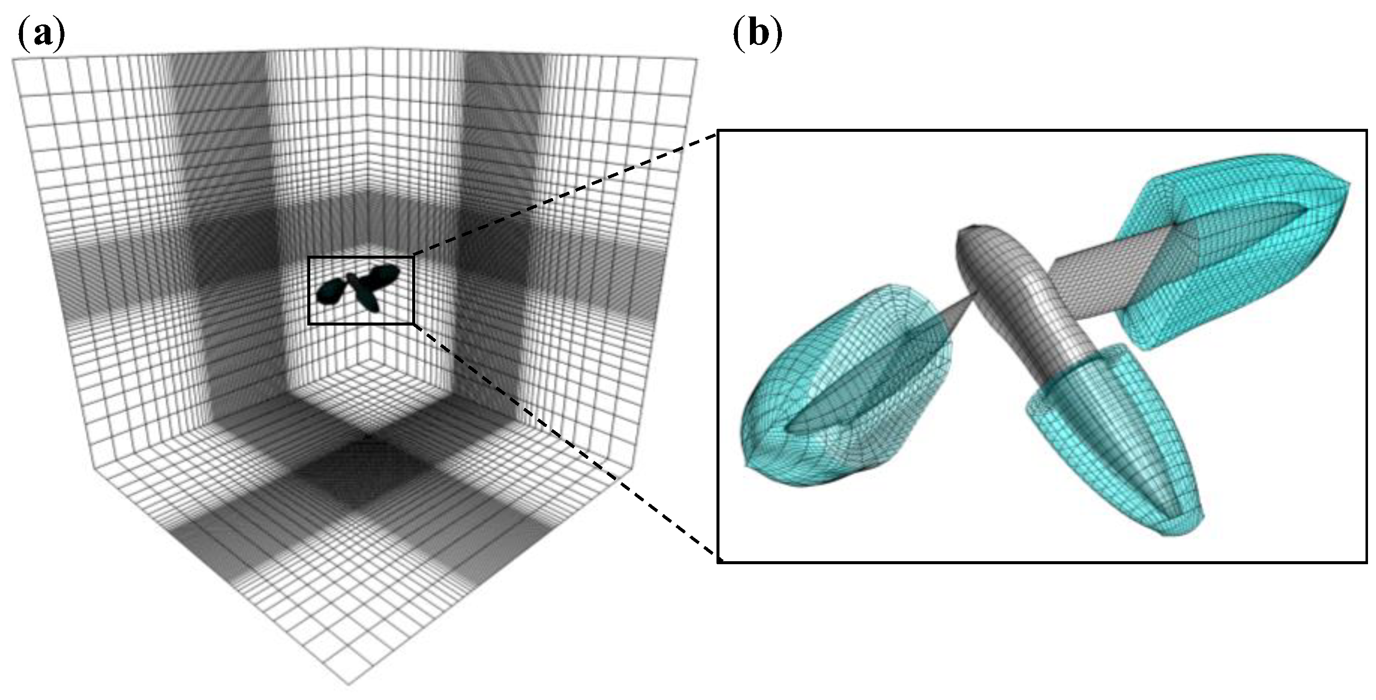
2.2. Numerical Model for Flow Field around a Flyer

For the analysis of the flow field around the hawkmoth model, we used a CFD solver based on a finite volume method and a fortified Navier–Stokes solver for a multi-blocked overset grid system [23]. The governing equations of the numerical solver are the three-dimensional incompressible unsteady Navier–Stokes equations written in strong conservation form for mass and momentum. The artificial compressibility method is used by adding a pseudo-time derivative of pressure to the equation of continuity. For an arbitrary deformable control volume V(t), the non-dimensionalized governing equations are

$${\int }_{V\left(t\right)}\left(\frac{\partial \mathit{Q}}{\partial t}+\frac{\partial \mathit{q}}{\partial \tau }\right)dV+{\int }_{V\left(t\right)}\left(\frac{\partial \mathit{F}}{\partial x}+\frac{\partial \mathit{G}}{\partial y}+\frac{\partial \mathit{H}}{\partial z}+\frac{\partial {\mathit{F}}_v}{\partial x}+\frac{\partial {\mathit{G}}_v}{\partial y}+\frac{\partial {\mathit{H}}_v}{\partial z}\right)dV=0,$$

(1)

where bold letters are used to denote matrices as

$$\begin{gathered} \mathit{Q}=\left[\begin{array}{c}u\\ v\\ w\\ 0\end{array}\right],\mathit{q}=\left[\begin{array}{c}u\\ v\\ w\\ p\end{array}\right],\mathit{F}=\left[\begin{array}{c}{u}^2+p\\ uv\\ uw\\ \lambda u\end{array}\right],\mathit{G}=\left[\begin{array}{c}vu\\ v^2+p\\ vw\\ \lambda v\end{array}\right],\mathit{H}=\left[\begin{array}{c}wu\\ wv\\ w^2+p\\ \lambda w\end{array}\right], \\ {\mathit{F}}_{\mathit{v}}=-\frac{1}{\mathrm{Re}}\left[\begin{array}{c}2u_x\\ u_y+v_x\\ u_z+w_x\\ 0\end{array}\right],{\mathit{G}}_{\mathit{v}}=-\frac{1}{\mathrm{Re}}\left[\begin{array}{c}{v}_{x+}{u}_y\\ 2v_x\\ v_z+w_y\\ 0\end{array}\right],{\mathit{H}}_{\mathit{v}}=-\frac{1}{\mathrm{Re}}\left[\begin{array}{c}{w}_{x+}{u}_z\\ w_{y+}{v}_z\\ 2w_z\\ 0\end{array}\right]. \end{gathered}$$

Above, λ is the pseudo-compressibility coefficient; p is pressure; u, v, and w are velocity components in the Cartesian coordinate system X, Y, and Z; t denotes physical time, while τ is pseudo-time; and Re is the Reynolds number. The term q associated with the pseudo-time is designed for an inter-iteration at each physical time step, which will vanish when the divergence of velocity is driven to zero to satisfy the equation of continuity. Reynolds number is defined as

$$Re=\frac{U_{ref}{L}_{ref}}{\nu },$$

(2)

where U_ref is a reference velocity, L_ref is a reference length, and ν is the kinematic viscosity of air. The forewing mean chord length is used as the reference length. The mean wingtip velocity of the forewing is used as the reference velocity; U_ref = U_tip = ωR, where R is the span length and ω is the mean angular velocity of the flapping wing (ω = 2Φf, where Φ is the wing positional angle amplitude and f is the flapping frequency). When we solve the Navier–Stokes equations for a wing block, the aerodynamic forces exerted on the wing are evaluated by a sum of inviscid and viscous flux over the wing surface as

$$F_{\mathrm{a}\mathrm{e}\mathrm{r}\mathrm{o}}\left(F_x,F_y,F_z\right)=-\sum _i^n\left({Flux}_{invis}+{Flux}_{vis}\right),$$

(3)

where n denotes the cell number on the surface of the wing. This CFD solver has been validated by comparison with some experimental studies, including the case of the hawkmoth wing [24].

In the present study, the computational domain was a Cartesian grid with 10R × 10R × 10R dimensions in which the body grid and the left- and right-wing grids (flyer blocks) were immersed (Figure 4). The Cartesian grid has two sub-regions: the clustering region, which has small uniform grid spacing, and the global region, which is gradually refined towards the center of the computational domain. The uniform grid spacing is set to 0.15 Cm in the model. The outer boundaries of the flyer blocks are immersed in the clustering region to prevent loss of accuracy due to the interpolation between the global block and flyer blocks. The numbers of grid points are the following: the global grid is 73 × 81 × 61; the body grid is 35 × 35 × 9; and the left- and right-wing grids are 45 × 45 × 15. The wing grids were clustered along the edges of the wing for higher resolution in the regions where strong shear flow is expected. The averaged grid size on the wing surface is approximately 0.045 Cm and 0.066 Cm in the chordwise and spanwise directions.

2.3. Wing Kinematics Modifications for Hovering Equilibrium Conditions

For the perturbation analysis of 3 degree-of-freedom (DoF) flight dynamics and passive dynamic stability, the hovering equilibrium conditions must be achieved. In this study, the body and wings are assumed as rigid models without considering the deformations, and the center of mass is calculated under the constant density distribution of the body and wings. The results of the computational aerodynamic forces using the wing kinematic model constructed based on the filming experiment described previously show that there are differences from the hovering equilibrium condition (i.e., the state in which the cycle-averaged values of the aerodynamic forces F_X, F_Z, and the aerodynamic torque T_Y are zero). Therefore, in this study, the following kinematic parameters were adjusted based on the previous studies [25,26] to achieve the hovering equilibrium conditions in 3 DoF flight dynamics—F_X: the amplitude center of the feathering angle; F_Z: flapping frequency; and T_Y: the center of mass in the Z-axis. Note that many insects have been observed to behave in a similar manner when their wings are damaged. For example, they often increase their flapping frequency to compensate for the reduction in wing area for the generation of lift (i.e., hawkmoth [27], damselfly [28], honeybee [29]).

Table 2. Tuning parameters and resultant forces for full-winged and forewing models.

	Measurement Model	Full-Winged Model	Forewing Model
Amplitude center of the feathering angle [deg]	7.36	11.86 (+4.5)	10.66 (+3.3)
Flapping frequency, f [Hz]	39.14	44.00 (+4.86)	45.70 (+6.56)
Center of mass in Z-axis [mm]	0	−5.29	−6.66
Cycle-averaged horizontal force, Fx [mN]	−1.13	−0.0019	0.012
Cycle-averaged vertical force, Fz [mN]	7.28	9.35	9.30
Total weight [mN]	9.38	9.38	9.28
Cycle-averaged pitching torque, Ty [mN·mm]	34.21	−0.011	0.017

shows the adjusted parameters and the resultant cycle-averaged aerodynamic forces and torques. Note that the measured value of the center of mass is set to zero as the initial position and that the values in parentheses are the deviation from the experimental results. The forewing model has a smaller wing area than the full-winged model, so the flapping frequency was increased to compensate for the lift force. The Reynolds number—Re of each tuning model was calculated by Equation (2)—is Re = 4392 for the full-winged model and Re = 3350 for the forewing model. Both models are on the order of 10³, and no significant difference in aerodynamic properties is expected.

2.4. Numerical Model for Flight Dynamics: Equations of 3 DoF Motions

In the present study, we treat the flyer as a bilaterally symmetric rigid model and investigate its 3 DoF motions in the longitudinal direction. In actual insect flight, the flapping motion of the wings causes a shift of the center of mass; however, because of its high frequency and the light mass of the wings in a hawkmoth, about 5 to 6% of the body [30], the morphological effect caused by the flapping motion is negligible compared with that of the body. Therefore, we assume that the center of mass is fixed and the moment of inertia of the body is constant regarding the body-fixed coordinate system for the treatment of the rigid body model [31]. Then, a single rigid body dynamic model can be reconstructed based on the Newton–Euler equations of 3 DoF motions as a set of three coupled nonlinear ordinary differential equations, such as

$$\begin{gathered} {\dot{u}}_b=-q_b·w_b+gsin\theta +\frac{F_{xb}}{m}, \\ {\dot{w}}_b=q_b·u_b-gcos\theta +\frac{F_{zb}}{m}, \\ {\dot{q}}_b=\frac{T_{yb}}{I_{yy}}, \end{gathered}$$

(4)

where F_xb and F_zb denote the aerodynamic forces acting along the x_b- and z_b- axes, respectively; T_yb is the aerodynamic pitching torque; θ is the pitch angle; u_b and w_b are the two components of the translational velocity of the body; q_b is the angular velocity of the body; and I_yy is the moment of inertia about the pitch axis of the body. Note that the translational and angular velocities of the body(u_b, w_b, q_b) are defined as three state variables that describe the 3 DoF motions in the body-fixed coordinate system. Body mass, m, moment of inertia, I_yy, and gravitational acceleration, g = 9.8 m/s², are assumed to be constant.

2.5. Nonlinear Stability Analysis Based on the Perturbation Theory

Gao et al. performed the passive dynamic stability analysis with a relatively small perturbation (i.e., the magnitudes of the vertical and horizontal disturbances were less than 5% of the cycle-averaged flapping velocity of the flyer) by applying the first-order approximation based on the assumption that the aerodynamic forces and torques vary linearly in the directions of the disturbances [32]. However, in the aerial environment of a flying insect, there are usually sharp velocity gradients and wing gusts and, hence, large disturbances [33]. Some studies have been conducted to analyze the nonlinear flight dynamics of hovering model insects by numerically solving the equations of motion coupled with Navier–Stokes equations to simulate large disturbance motions [34], but these studies are computationally expensive. Therefore, in the present study, considering that the aerodynamic forces are on the scale of the square of the reference velocity, the second-order approximation is implemented to express the differences on the aerodynamic forces and torque with the perturbations. The construction is as follows.

First, a function representing aerodynamic forces and torque is defined and constructed in the form of a Fourier series, considering four conditions—one equilibrium condition and three unidirectional perturbation conditions. Under equilibrium conditions, time-varying aerodynamic forces and moments based on the CFD model can be decomposed into a Fourier series for a complete wing beat cycle [35], in the form of

$$F(t)=\sum _{n=0}^h(a_n\cos \left(nkt\right)+b_n\sin \left(nkt\right)),$$

(5)

where k is the reduced frequency; a_n and b_n are Fourier series coefficients. Note that the coefficient, a₀ represents the cycle-average aerodynamic force or torque over a single flapping cycle. The higher the harmonic h, the better this function fits the original value. In the present study, the tenth-order Fourier series (h = 10) was found to be sufficient for reproducing all the waveforms of the aerodynamic forces and torque generated by the CFD solver.

Second, considering that the perturbation conditions are achieved by specifying the deviation of the translational velocity and angular velocity of the body, the function in Equation (5) should change with both time t and time-varying state variables. Therefore, it is necessary to construct a system function in terms of these four variables (t, u_b, w_b, q_b) to solve the equations of motion in Equation (4) while updating the time-varying aerodynamic forces and torque. To construct this system function, a CFD solver was utilized to obtain the aerodynamic forces and torque under the perturbation conditions in three directions. For the horizontal direction, the dimensionless translational velocity was given as eight different perturbation conditions in the range −1.0 < u < 1.0, as well as w for the vertical direction. For the pitch direction, the dimensionless angular velocity was given as six perturbations in the range −0.05 < q < 0.05. Note that u and w are the dimensionless inflow velocities in the X- and Z-axes. Using these results, the aerodynamic forces and torque under the perturbation conditions are approximated by introducing a quadratic function, such as

$$\left[\begin{array}{c}{F}_x\\ F_z\\ T_y\end{array}\right]=\left[\begin{array}{c}{F}_{xe}\\ F_{ze}\\ T_{ye}\end{array}\right]+\left[\begin{array}{ccc}{C}_{F_x,u}& C_{F_x,w}& C_{F_X,q}\\ C_{F_z,u}& C_{F_z,w}& C_{F_z,q}\\ C_{T_y,u}& C_{T_y,w}& C_{T_y,q}\end{array}\right]·\left[\begin{array}{c}u\\ w\\ q\end{array}\right]+\left[\begin{array}{ccc}{D}_{F_x,u}& D_{F_x,w}& D_{F_X,q}\\ D_{F_z,u}& D_{F_z,w}& D_{F_z,q}\\ D_{T_y,u}& D_{T_y,w}& D_{T_y,q}\end{array}\right]·\left[\begin{array}{c}{u}^2\\ w^2\\ q^2\end{array}\right],$$

(6)

where

$$\begin{gathered} \left[\begin{array}{c}{F}_{xe}\\ F_{ze}\\ T_{ye}\end{array}\right]=\sum _{n=0}^{10}\left(a_{i,n}\cos \left(n\omega t\right)+b_{i,n}\sin \left(n\omega t\right)\right), \\ {C}_{i,j}=\sum _{n=0}^{10}\left(c_{i,j,n}\cos \left(n\omega t\right)+d_{i,j,n}\sin \left(n\omega t\right)\right), \\ {D}_{i,j}=\sum _{n=0}^{10}(e_{i,j,n}\cos \left(n\omega t\right)+f_{i,j,n}\sin \left(n\omega t\right)). \end{gathered}$$

Above, the forces and torque (F_xe, F_ze, T_ye) are obtained under the trimmed flight condition without perturbation (see Section 2.3); ω is the angular frequency of the wing beat; a~f are Fourier series coefficients; the subscript of i denotes the aerodynamic force and torque components and j denotes the perturbation components.

At this stage, the solution of Equation (6) is transformed to the body-fixed coordinate system, yielding F_xb, F_zb, and T_yb which can be utilized for Equation (4). Finally, it was possible to simulate the state variables under the perturbation conditions by performing the time integration while inserting the perturbations obtained from Equation (4) into Equation (6) at each time step.

3. Results and Discussion

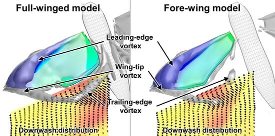
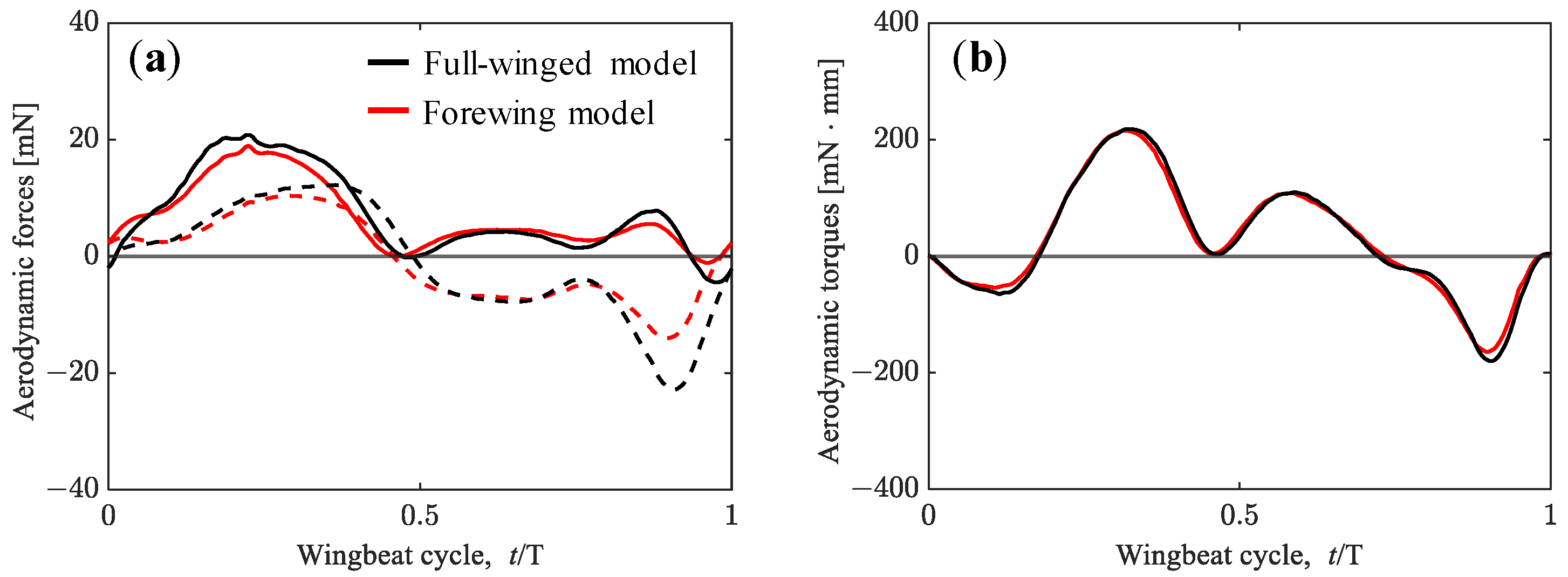
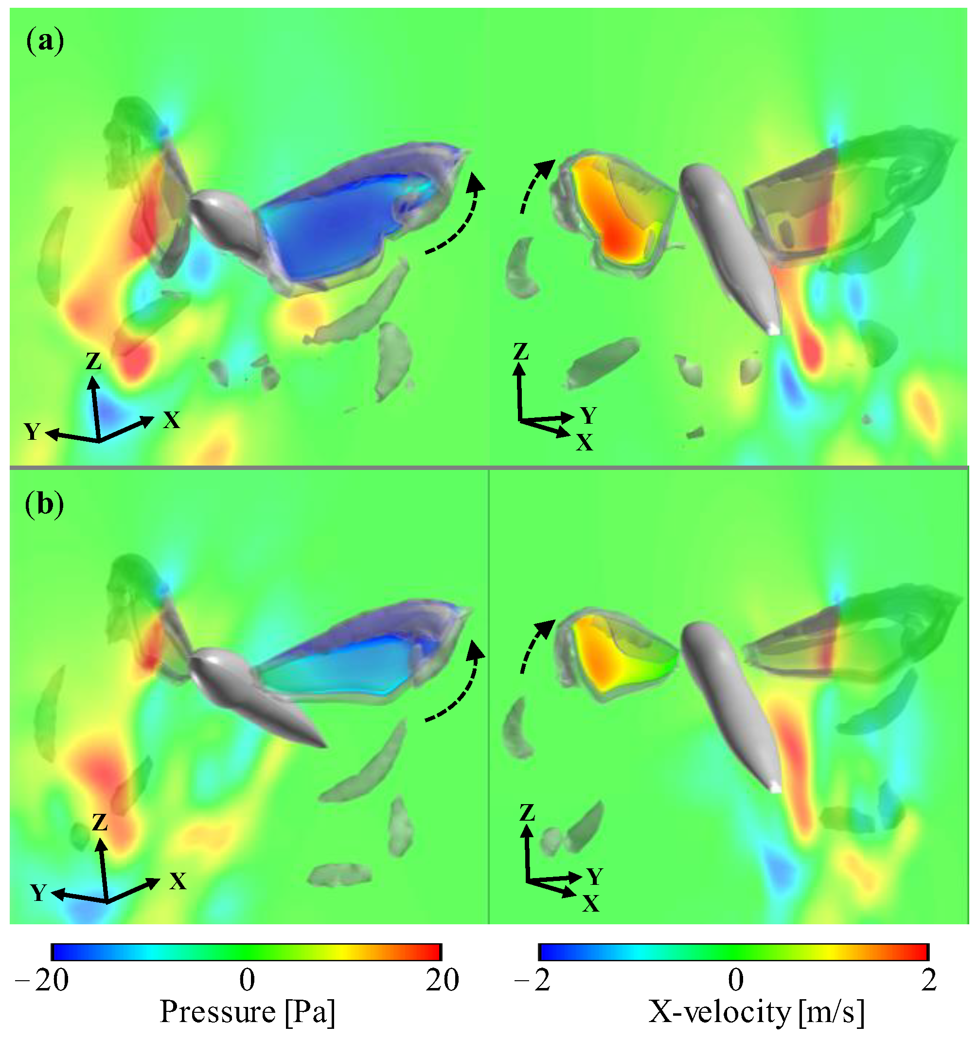
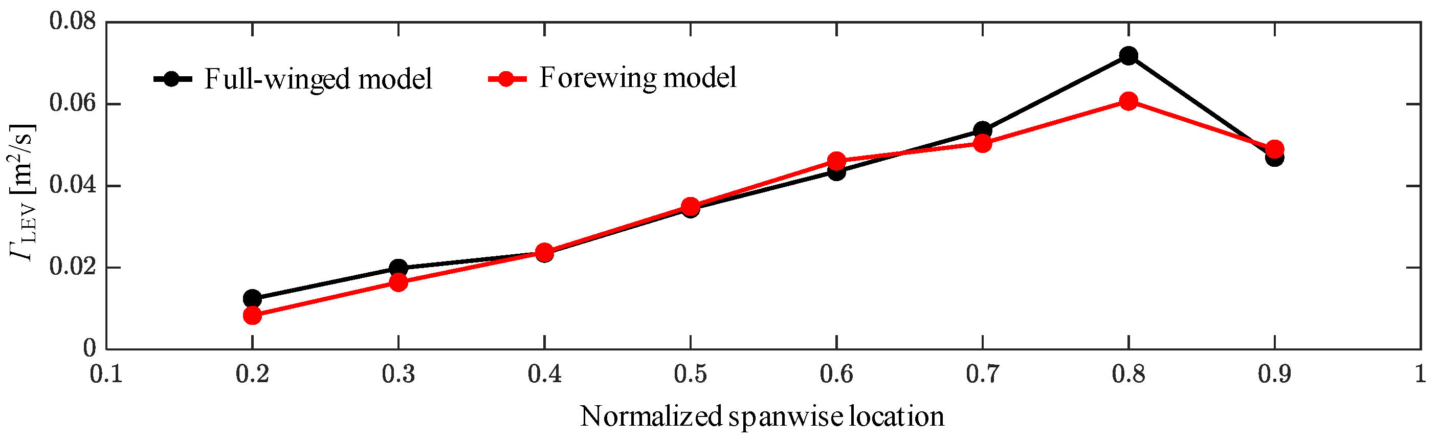
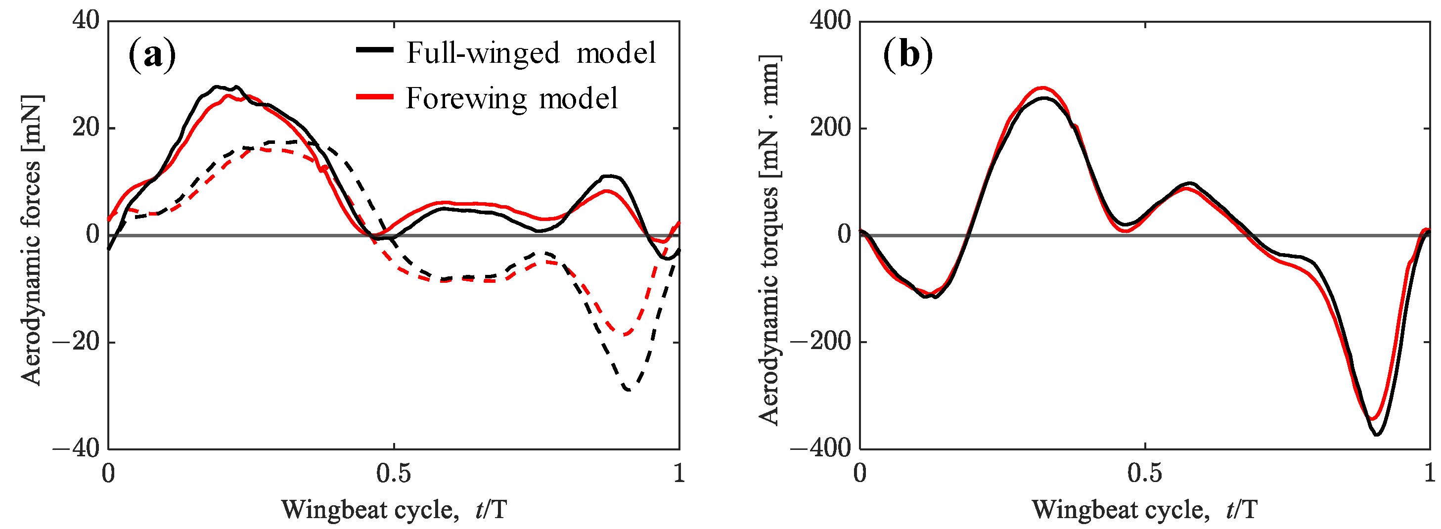
3.1. Aerodynamic Performance of a Hawkmoth with/without Hindwings

First, to clarify the effects of the hindwings on the aerodynamic performance of the hovering hawkmoth, we performed the numerical simulation of the full-winged and forewing models by adopting the measured wing kinematics (Figure 3). The difference between these two models here is the wing area; the wing area of the forewing model is about 73% of that of the full-winged model. Regarding force production, it is known that the force generated by a flapping or revolving wing is proportional to the second moment of the wing area [36]. In the present study, the second moment of the wing area can be calculated as

$$S={\int }_0^R{C}_m\left(r\right)r^{2}dr,$$

(7)

where r denotes the spanwise location of the local wing element. The second moment of the wing area of the forewing model results in 93% of that of the full-winged model. The vertical and horizontal aerodynamic forces and pitching torque during a wingbeat cycle are depicted in Figure 5, and the cycle-averaged aerodynamic forces, wing area (refer again as in Table 1), and the second moment of wing area are summarized in

Table 3. The cycle-averaged forces, torque, and the wing parameters.

	Full-Winged Model	Forewing Model
Cycle-averaged horizontal force, Fx [mN]	−1.13	−0.80 (70%)
Cycle-averaged vertical force, Fz [mN]	7.28	6.73 (93%)
Cycle-averaged pitching torque, Ty [mN·mm]	34.21	28.53 (85%)
Wing area [mm2]	443	325 (73%)
Second moment of wing area [mm4]	1.41 × 10−7	1.31 × 10−7 (93%)

. The values in parentheses for the forewing model indicate the percentages compared with the full-winged model.

The considerable difference in aerodynamic forces between the full-winged and forewing models can be seen in the timing around t/T = 0.9. At this timing, the wings are flapping with a geometric angle of attack close to 90 degrees, generating the large positive pressure region on the upper surface and the large negative pressure region on the lower surface, resulting in a large drag-based thrust (Figure 6). This thrust is greater in the full-winged model which has a longer chord length than the forewing model, and the positive velocity increase in the X-axis can be seen in the visualized X-velocity distributions around the wings.

In terms of lift force during downstroke, the full-winged model maintains a greater lift force than the forewing model at approximately a constant rate, and the average values of lift force during downstroke are 11.79 and 10.18 [mN], respectively. The delayed stall of the leading-edge vortex (LEV) on the wing surface during the flapping motion has been observed [3,37,38,39], and it can promote the lift force. The presence of the LEV on the wing surface creates a relatively low-pressure region, which increases the lift force. To clarify the differences in lift force in the present study, we quantified the strength (circulation) of the LEV at t/T = 0.2, where the maximum lift forces occur in both models. The LEV circulation was estimated by integrating the vorticity as follows.

$${\Gamma }_{LEV}={\iint }_S^{}\omega ·dS,$$

(8)

where ω is the vorticity. Note that the area of integration, dS, is bound by the vorticity threshold for capturing the LEV (25% of the peak vorticity in this study) as in [40]. The spanwise distributions of the instantaneous LEV circulation at t/T = 0.2 are shown in Figure 7. In both the full-winged and forewing models, the LEV intensities increase linearly with almost the same slope from the wing root to 0.8R at the wingtip. Chen et al. adopted a revolving wing model of a hawkmoth and reported that LEV formation is almost the same when the hindwings are removed, and thus, the forewings can produce most of the aerodynamic forces [41], indicating that the results adopting the flapping kinematics in the present study show similar results for LEV formation. The decrease in the values at 0.9R is caused by the interference of the wing tip vortex. The only considerable difference occurs in the circulation at 0.8R, where the full-winged model shows about an 18% increase compared with the forewing model. Phillips et al. performed the experiments with simple rectangular wings and insect kinematics and reported more enhanced LEV circulation across the span with an increasing aspect ratio (AR) [10]. On the other hand, Harbig et al. reported in their numerical calculations of a revolving wing with a fruit fly model that the narrower width per unit span of a high-AR wing causes the LEV to interact with the trailing-edge vortex (TEV) from the lower side of the wing, reducing the circulation and, thus, the lift [42]. Comparing cicada hindwings with hindwing-less Drosophila, in which the cicada wings have two distinct trailing-edge shapes with a reduced wing tip area and an increased wing root area, clear differences in trailing-edge vortex formulation and stabilization of the flow in the wing span direction have been reported to improve lift [43]. The difference in TEV structure was also observed in the present study (Figure 8), where the TEV of the forewing model was more backwardly tilted along its trailing-edge shape around the wing root compared with the full-winged model, and it shed from the wing surface earlier than the full-winged model. The local difference in LEV intensity between the full-winged and forewing models when the area is reduced only on the wing root side, as in this study, may not be due to the effect of AR but rather to the difference in the trailing-edge vortex. In addition, the difference in the vertical velocity distributions (Figure 8) indicates that the downwash is more widely spread on the wing root side in the full-winged model than in the forewing model, resulting in greater lift near the wing root as well. Because the wingtip vortices in both models do not show significant differences, this may not be caused by a change in the relative angle of attack due to the downward velocity induced by the wingtip vortices, but rather, it is due to the fact that the TEV remains distinct near the trailing edge, as seen in Figure 8 and in the longer chord length in the full-winged model. It is also possible that the spread of downwash in the wing root region may enhance the stability of the LEV, as seen in the circulation at 0.8R [44,45,46].

In flapping flight, the cycle-averaged aerodynamic force-to-power ratio (F_Σ/P) can be utilized for estimating the efficiency [47]. The aerodynamic power imparted to the air by each wing is defined as

$$P=-\sum _i^N\left(F_{aero,i}·v_{surf,i}\right),$$

(9)

where N denotes the number of elements on the surface of each wing; F_aero is the aerodynamic force acting on each element; and v_surf is the corresponding velocity of each element. The efficiencies of the left and right wings in generating lift force are 19.5% for the full-winged model and 22.8% for the forewing model, with the forewing model being slightly more efficient. Similarly, numerical results using a revolving hawkmoth wing model with/without hindwings reported improved aerodynamic efficiency of a forewing model [41]. In the comparison of the cycle-averaged values, 30% and 7% reductions in horizontal and vertical forces are observed due to the reduction in wing area. From the morphological parameters of the wings in Table 3, the reduction of the horizontal force in the forewing model is almost equal to the reduction ratio of the wing area (=27%), and the reduction of the vertical force is almost identical to the reduction of the second moment of the wing area (=7%). The cycle-averaged aerodynamic torque was slightly higher in the pitch-up direction for the full-winged model. This may be caused by the moving of the center of the air pressure closer to the center of mass in the forewing model.

The aerodynamic forces obtained from trimmed flight by adopting the tuned wing kinematics for the full-winged and forewing models are shown in Figure 9. The differences in the wing kinematics that affect the aerodynamic force generation in both models are the flapping frequency and the amplitude center of the feathering angle, which differ by 1.7 Hz and 1.2°, respectively (see Table 2). While the maximum lift and thrust increased with increasing flapping frequency in the tuned wing kinematic models, the waveforms of the aerodynamic forces and torque were similar to those of the measured wing kinematic models for both the full-winged and forewing models (Figure 5 vs. Figure 9). For the models with the tuned wing kinematics here, the cycle-averaged values of the aerodynamic horizontal force and the aerodynamic torque in the pitch direction were close to zero, and the vertical aerodynamic force is nearly balanced by its own weight, indicating that a state close to trimmed flight was achieved (Table 2).

3.2. Hovering Equilibrium Condition

As discussed in previous studies [32], the initial values of aerodynamic forces and torque in the flight dynamic analysis have a significant effect on the subsequent dynamic behavior, and thus, the initial time of the dynamic analysis must be adjusted to achieve a long-term hovering equilibrium condition in the absence of active control of the wing motion. As a result of the parameter study, appropriate initial times of t₀ = 0.3574 and 0.3487 were obtained for the full-winged and forewing models. With these initial times, the equilibrium conditions are achieved up to 20 beat cycles and the time variation of the state variables u_b, w_b and q_b oscillate in a range of −0.016 < u_b < 0.006, −0.016 < w_b < 0.001, and −0.013 < q_b < 0.010 for the full-winged model and −0.015 < u_b < 0.006, −0.013 < w_b < 0.001, and −0.008 < q_b < 0.007 for the forewing model (Figure 10). In the present study, these equilibrium conditions were defined as stable hovering flight, and then the dynamic analysis was performed by adding the various perturbations.

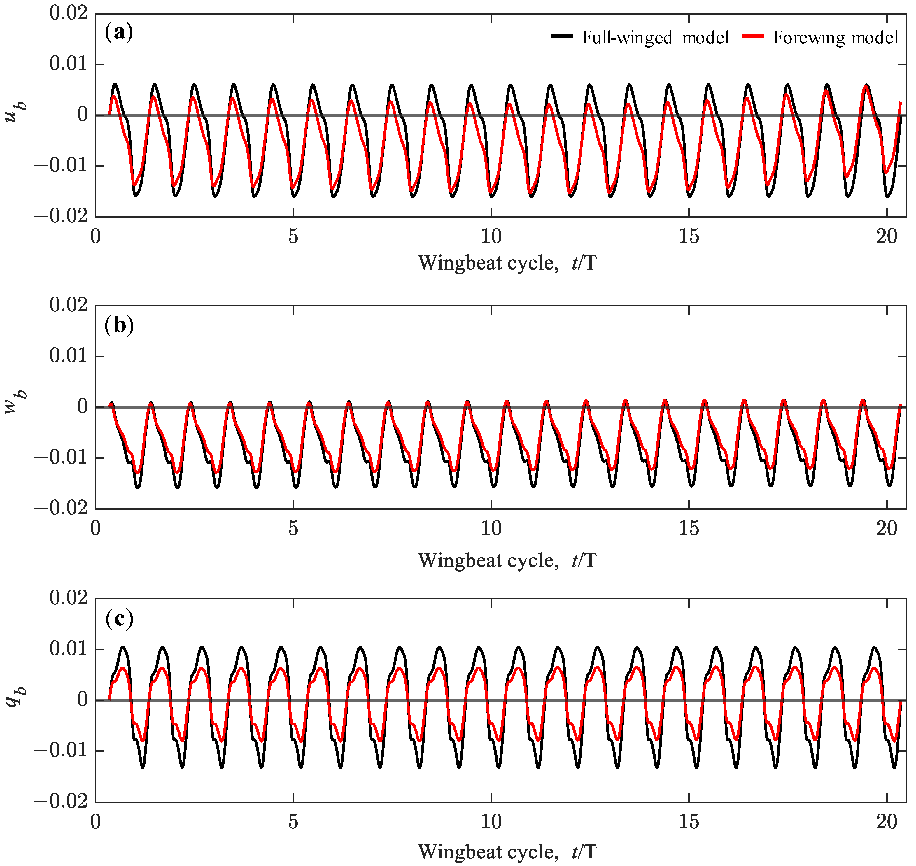
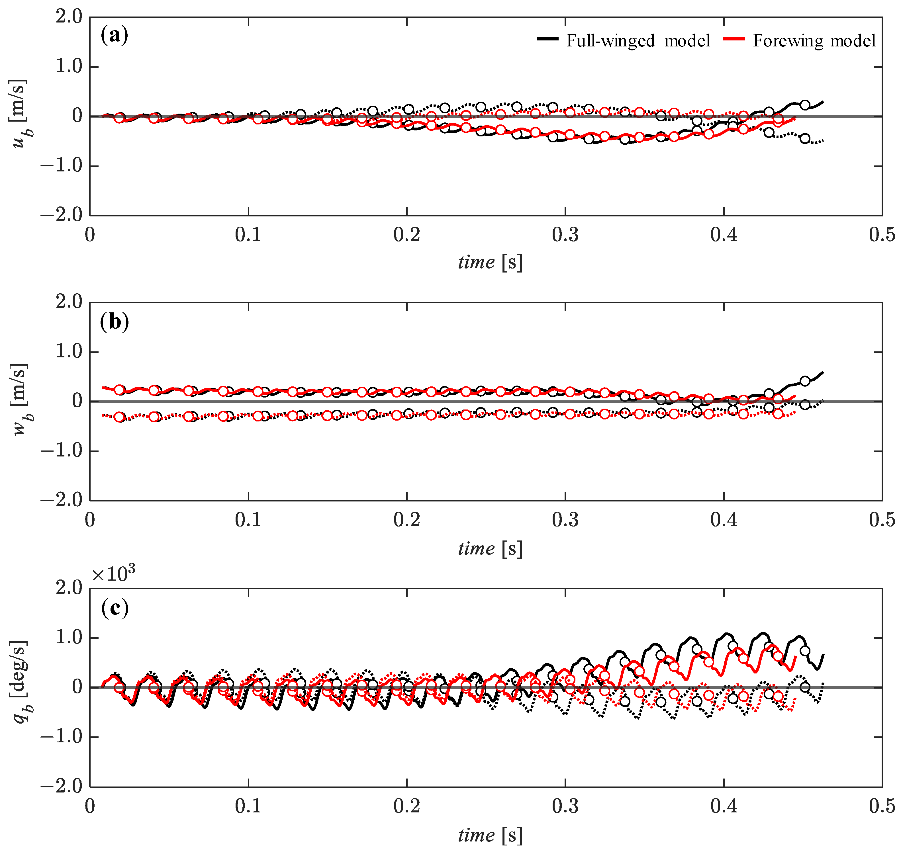
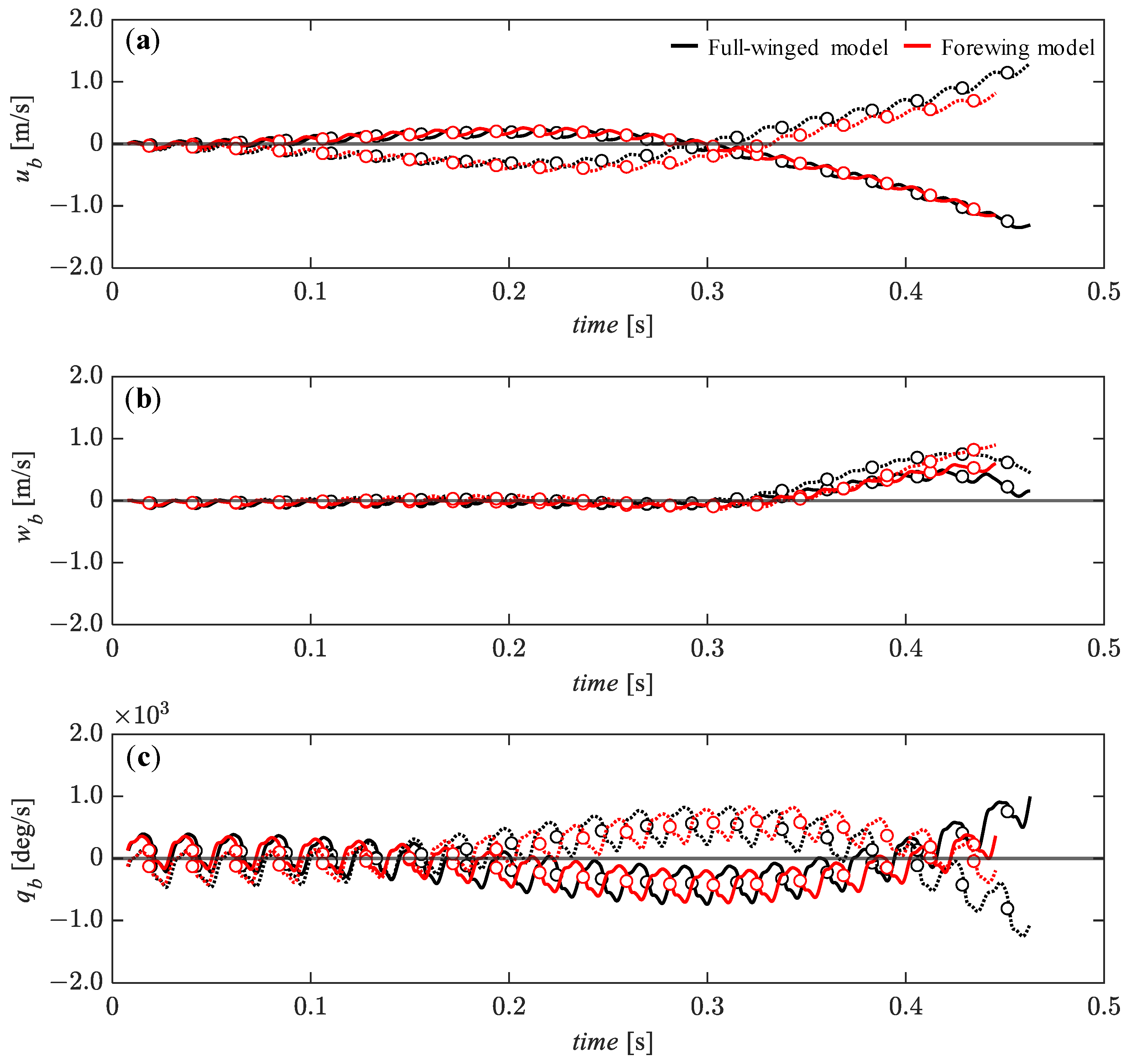
3.3. Passive Dynamic Stability with Relative Small Perturbations

In this section, the dynamic analysis was performed under relatively small perturbations—5% of the reference velocity for the u_b and w_b components and 0.5% of the reference angular velocity for the q_b. Figure 11 presents the time histories of the state variables under the initial conditions of u_b = 0.05 (solid line) and u_b = −0.05 (dashed line). It can be seen that the x_b-axial velocity component (u_b) converges monotonically and gradually to an equilibrium state up to about t = 0.15 [s] (Figure 11a) while the z_b-axial velocity component (w_b) remains in an equilibrium condition (Figure 11b). The pitch angular velocity, q_b tends to gradually diverge up to this time, but after t = 0.15 [s], it gradually converges to an equilibrium state until about t = 0.25 [s] (Figure 11c) while the u_b and w_b tend to diverge during this time. The pitch-up motion (q_b is positive) due to the forward perturbation (u_b = −0.05) and the pitch-down motion (q_b is negative) due to the backward perturbation (u_b = 0.05) during the first few flapping cycles are similar in trend to the passive response of Drosophila with a high aspect ratio wing [32]. This passive response is likely to promote convergence because the pitch-up/down motion leads to a modulation of increased backward/forward aerodynamic forces [48], which can passively reduce the forward/backward deviation. There is no significant difference depending on the presence or absence of hindwings, but the u_b and w_b recover to a transient equilibrium state slightly earlier in the full-winged model than in the forewing model.

For the vertical initial perturbations of w_b = 0.05 (solid line) and w_b = −0.05 (dashed line), it can be seen that the overall transitions of the state variables are more stable than for the horizontal perturbations (Figure 11 vs. Figure 12). Although there is a slight divergence trend in the u_b (Figure 12a), all state variables remain stable up to about t = 0.25 [s]. In particular, for the w_b, the passive restoring force acts steadily and monotonically up to about t = 0.4 [s] (Figure 12b). After t = 0.25 [s], the u_b and the pitch angular velocity, q_b are more stable for the downward perturbation than for the upward perturbation, with the same trend for both full-winged and forewing models. The difference between the full-winged and the forewing models can be seen in the pitch angular velocity after t = 0.3 [s] (Figure 12c). The forewing model is able to delay the divergence trend for the upward perturbation compared with the full-winged model. The stable behavior of the translational velocity and the development of the pitch instability in response to the vertical perturbations in both models are similar to those observed in the analysis of nonlinear flight dynamics with the fully coupled Navier–Stokes equation and the equation of motion [34].

With respect to the pitch perturbations, there is a slightly more stable transition for the u_b around t = 0.1 to 0.3 [s] for the pitch-up (solid lines) perturbation compared with the pitch-down (dashed line) perturbation (Figure 13a), and this trend is also observed for the pitch angular velocity, q_b around t = 0.2 to 0.4 [s] (Figure 13c). The w_b is less affected by the pitch perturbation and remains in the equilibrium state until about t = 0.3 [s] (Figure 13b) when the u_b starts to diverge significantly at this timing. Although there is no significant difference between the full-winged and the forewing models, the u_b and w_b around t = 0.3 to 0.4 [s] under the pitch-down perturbation have a slightly smaller slope in the positive direction for the forewing model than for the full-winged model, indicating that the forewing model is less affected by the pitch perturbations.

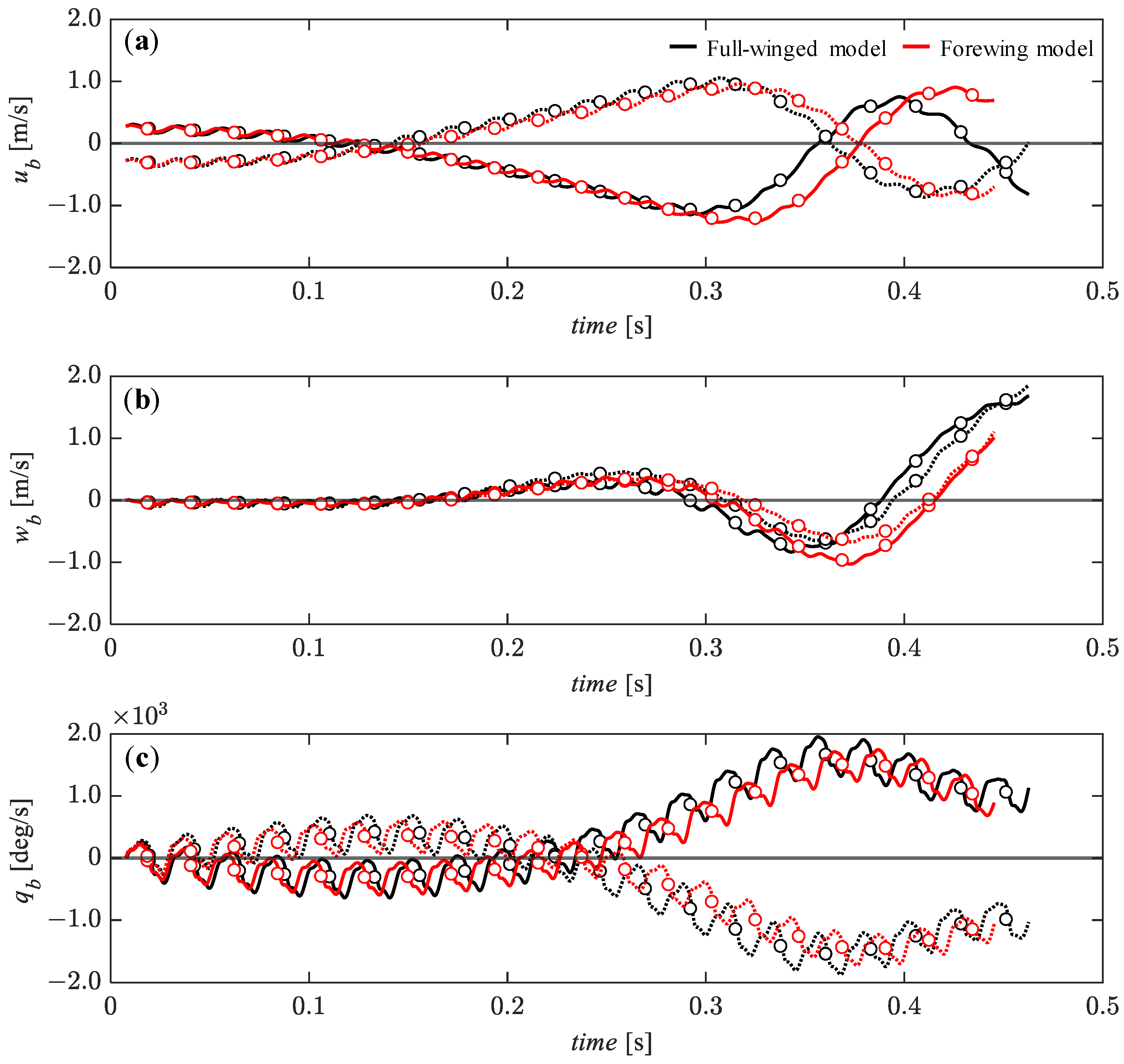
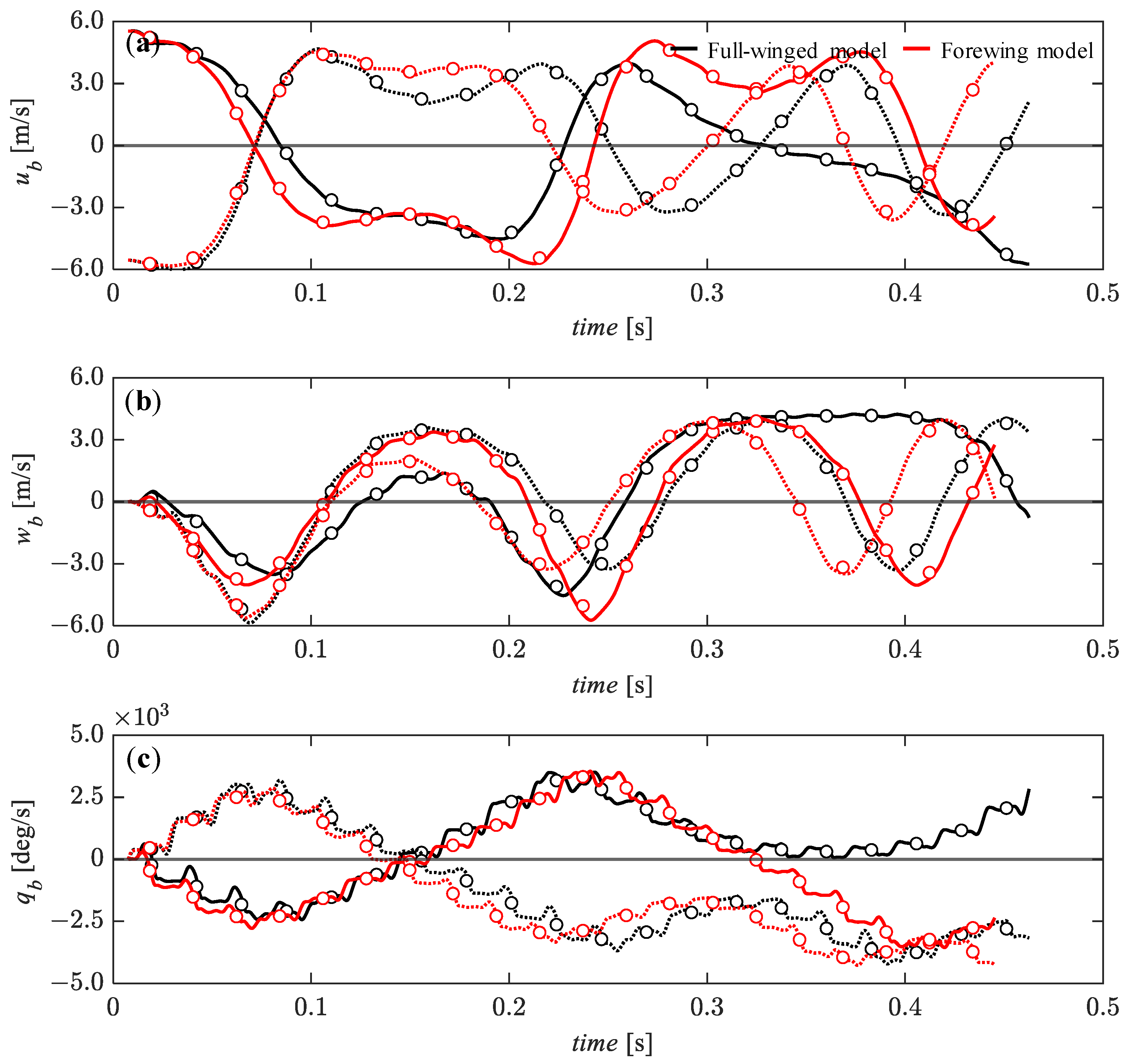
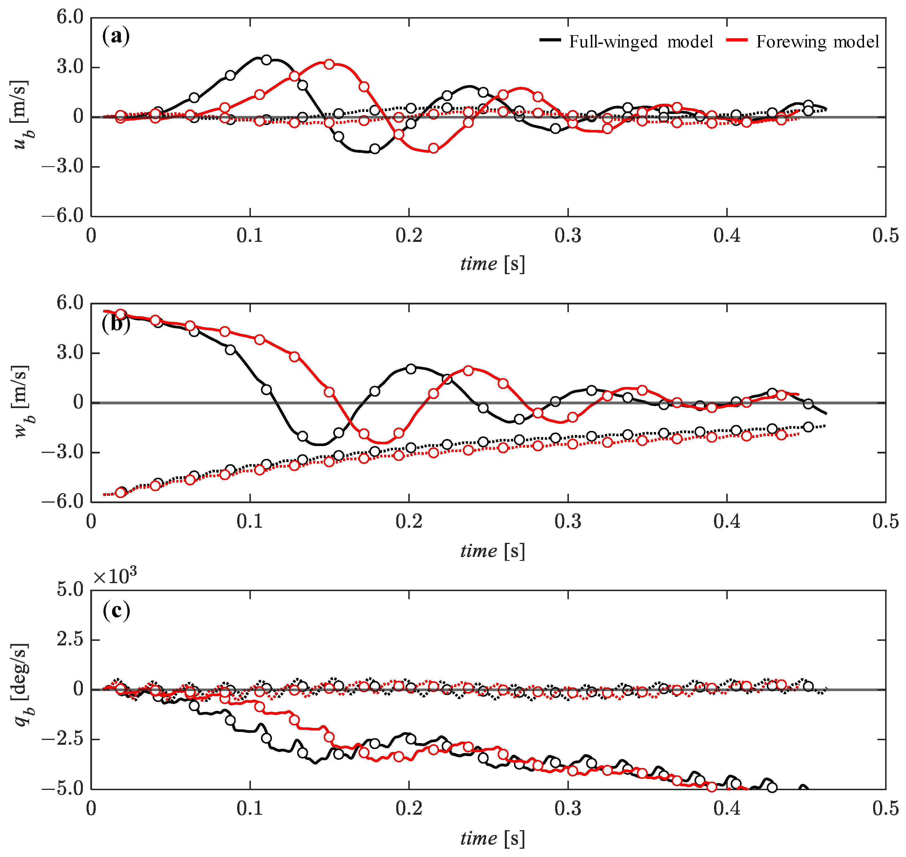
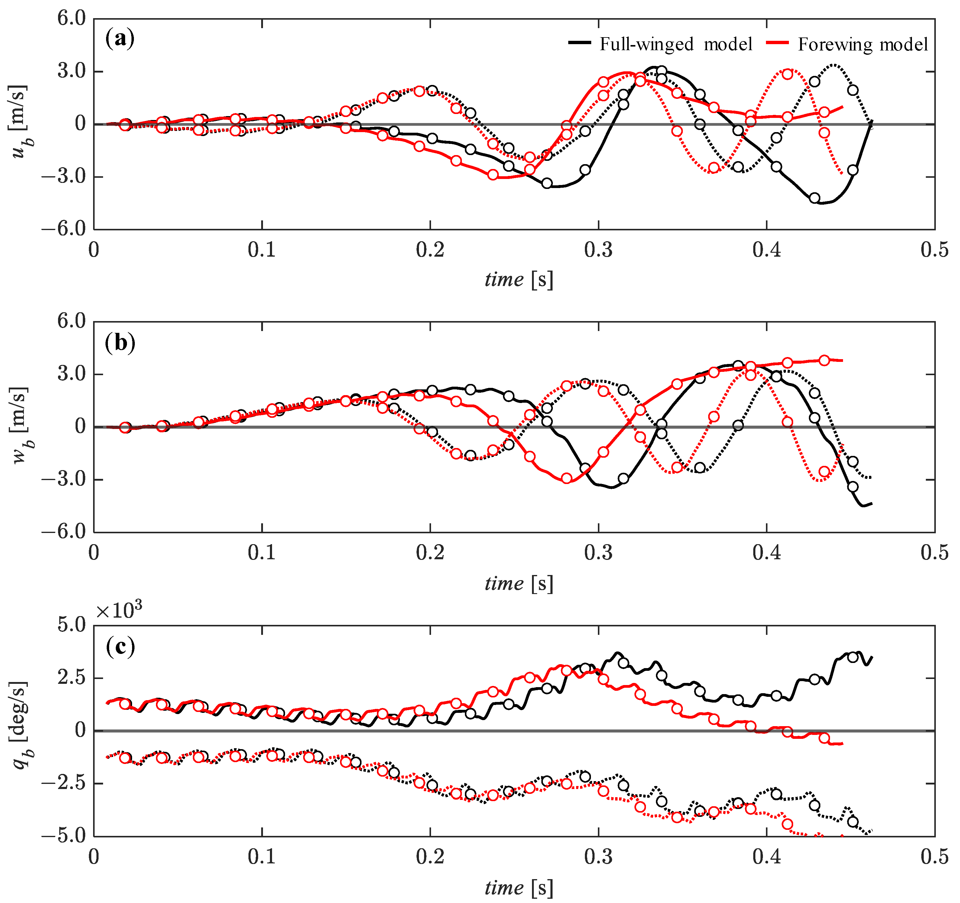
3.4. Passive Dynamic Stability with Relatively Large Perturbations

Here, we present the response of the state variables to the large perturbations—100% of the reference velocity for the u_b and w_b components and 5% of the reference angular velocity for the q_b. For the forward and backward perturbations of the u_b, the response of the u_b tends to converge during the first few flapping cycles as in the case of a small perturbation of the u_b (Figure 11a and Figure 14a), while the w_b and pitch angular velocity, q_b diverge significantly during this period (Figure 14b,c). Note that the response of the pitch angular velocity, q_b during the first three cycles acts to passively reduce the forward/backward deviation, as in the case of the small perturbation of the u_b. Thereafter, the large monotonic oscillations tend to begin in all state variables. After t = 0.32 [s], the full-winged and forewing models show differences in response to the backward perturbation with the forewing model continuing the large oscillations in all state variables while the full-winged model shows different behavior. The full-winged model shows stable behavior with respect to the u_b and the pitch angular velocity, q_b maintaining an almost equilibrium state for a short period.

The most stable passive restoring forces in the present study were found in the response of the u_b and w_b to large vertical perturbations (Figure 15a,b). For the upward perturbation (solid lines), the u_b initially diverges in a positive direction but then becomes a damped oscillation, similar to the response of the w_b; finally, both values recover to an equilibrium state in about t = 0.4 [s]. For the downward perturbation (dashed lines), the u_b is almost unaffected and remains in the equilibrium state, as in the case of the small perturbation (Figure 12a and Figure 15a), while the w_b shifts monotonically and gradually from the initial perturbation values to an equilibrium state (Figure 15b). The pitch angular velocity, q_b has little effect for the downward perturbation but is significantly shifted away from the equilibrium state for the upward perturbation (Figure 15c). This clear difference in the pitch instability due to the directions of the large vertical perturbations is also observed in the previous study [34]. Under the large vertical perturbation, the differences in the response of the state variables between the full-winged and forewing models were observed that were not seen under the small perturbation. In the full-winged model, the u_b, the w_b, and the pitch angular velocity, q_b are all more sensitive to the upward perturbation than in the forewing model, indicating that the presence of hindwings has a greater effect in this case.

With respect to the pitch perturbation, the u_b and the pitch angular velocity, q_b tend to converge to the equilibrium state until about t = 0.1 [s], but thereafter all state variables oscillate significantly by increasing the w_b, and the amplitude tends to increase with time. As seen in the response to the large perturbation in the u_b, after t = 0.32 [s], the full-winged and forewing models show the difference in response to this pitch perturbation (Figure 14 and Figure 16). The full-winged model continues to oscillate significantly for all state variables while the forewing model shows the behavior that breaks the periodic motion at this time. The forewing model shows a gradual convergence to the equilibrium state with respect to u_b and pitch angular velocity, q_b until about t = 0.4 [s].

These behaviors show that the full-winged model is partially stable for the horizontal perturbation while the forewing model is partially stable for the pitch perturbation, indicating that the hindwing can act for better or worse depending on the direction of the perturbation.

3.5. Effect of Hindwings on Passive Dynamic Stability

The results of the passive dynamic stability analysis with the hawkmoth in the present study showed that for some perturbations, the state variables converged to the equilibrium state condition as reported in the study on the longitudinal dynamic stability of a hawkmoth adopting a linear time-invariant dynamic model [34], but for other perturbations, an inherent instability was observed as reported for the desert locust and the bumblebee in the open-loop conditions with a linear theory [15,49]. There are some small differences in flight behavior with/without hindwings in the present study, but no clear trend was observed. In nature, insects suffer wing damage throughout their lives [50], but even if they have lost or damaged their hindwings, most of them can still fly, so the intrinsic influence of hindwings on passive flight stability may be small. However, in terms of flight maneuverability, in the flights of moths and butterflies (Lymantria dispar and Pieris rapae) with severed hindwings, which have a larger ratio of hindwings to total wing area than the model in this study, a reduction in flight maneuverability in terms of linear and turning acceleration has been reported as a result of hindwing resection [20]. In the escape flights of moths with varying hindwing shapes in response to bat predation, it was reported that species with longer hindwings in the chordwise direction were more successful in deflecting predation by bats [51]. Flying insects are known to adopt flight strategies that actively modify wing kinematic parameters, such as flapping frequency, flapping amplitude, and stroke plane angle [27,28,29], when wing area is reduced due to wing damage. In terms of passive flight stability, it has been reported that wing flexibility can improve flight stability [52]. It should be noted that a comprehensive evaluation of the unique impact of hindwings on flight stability in natural insects may be possible by considering active changes in wing kinematics and passive wing deformation, which were not considered in this study.

The delay in controlling active wing motion in insects is estimated to be several flapping cycles [14], and the results of passive flight behavior in this study for the long flapping cycles may not necessarily be related to the flight behavior of actual insects; however, this study does play a great role in considering the wing design in FMAVs. In particular, the presented results may be useful to guide the design of wings in terms of whether to adopt wings with a high aspect ratio to improve flight maneuverability, or wings with a small aspect ratio and a large wing root area to achieve a high passive response and damped vibration during the first few flapping cycles to perturbations.

4. Conclusions

In the present study, we investigated the aerodynamic effects and passive dynamic stability with/without hindwings in the hawkmoth, Agrius convoluvuli. In terms of aerodynamic effects, it was suggested that the hindwings may contribute to the enhancement of partial LEV circulation during downstrokes due to the stable TEV of the hindwings. An increase in downwash at the hindwings was also observed while the hindwings have a slight negative effect on the efficiency of lift generation. For thrust generation, a significant increase was observed in the region of the hindwings during upstrokes. In terms of passive dynamic stability, the results showed that the presence or absence of the hindwings did not show a significant trend, but the hindwings may contribute to improving flight stability depending on the direction of any perturbations. The results obtained in this study may be useful for the integrated development of wing geometry and flight control for FMAVs.

References

1. Rothstein, A. Drone; Bloomsbury Publishing: New York, NY, USA, 2015. [Google Scholar]
2. Floreano, D.; Wood, R.J. Science, Technology and the Future of Small Autonomous Drones. Nature 2015, 521, 460–466. [Google Scholar] [CrossRef]
3. Ellington, C.P.; Van Den Berg, C.; Willmott, A.P.; Thomas, A.L. Leading-Edge Vortices in Insect Flight. Nature 1996, 384, 626–630. [Google Scholar] [CrossRef]
4. Dickinson, M.H.; Lehmann, F.-O.; Sane, S.P. Wing Rotation and the Aerodynamic Basis of Insect Flight. Science 1999, 284, 1954–1960. [Google Scholar] [CrossRef]
5. Sane, S.P. The Aerodynamics of Insect Flight. J. Exp. Biol. 2003, 206, 4191–4208. [Google Scholar] [CrossRef]
6. Chin, D.D.; Lentink, D. Flapping Wing Aerodynamics: From Insects to Vertebrates. J. Exp. Biol. 2016, 219, 920–932. [Google Scholar] [CrossRef]
7. Sane, S.P.; Dickinson, M.H. The Aerodynamic Effects of Wing Rotation and a Revised Quasi-Steady Model of Flapping Flight. J. Exp. Biol. 2002, 205, 1087–1096. [Google Scholar] [CrossRef]
8. Li, H.; Nabawy, M.R. Effects of Stroke Amplitude and Wing Planform on the Aerodynamic Performance of Hovering Flapping Wings. Aerospace 2022, 9, 479. [Google Scholar] [CrossRef]
9. Phillips, N.; Knowles, K.; Bomphrey, R.J. Petiolate Wings: Effects on the Leading-Edge Vortex in Flapping Flight. Interface Focus 2017, 7, 20160084. [Google Scholar] [CrossRef]
10. Phillips, N.; Knowles, K.; Bomphrey, R.J. The Effect of Aspect Ratio on the Leading-Edge Vortex over an Insect-like Flapping Wing. Bioinspir. Biomim. 2015, 10, 056020. [Google Scholar] [CrossRef]
11. Berman, G.J.; Wang, Z.J. Energy-Minimizing Kinematics in Hovering Insect Flight. J. Fluid Mech. 2007, 582, 153–168. [Google Scholar] [CrossRef]
12. Nabawy, M.R.; Crowther, W.J. Optimum Hovering Wing Planform. J. Theor. Biol. 2016, 406, 187–191. [Google Scholar] [CrossRef]
13. Taylor, G.K. Mechanics and Aerodynamics of Insect Flight Control. Biol. Rev. 2001, 76, 449–471. [Google Scholar] [CrossRef]
14. Elzinga, M.J.; Dickson, W.B.; Dickinson, M.H. The Influence of Sensory Delay on the Yaw Dynamics of a Flapping Insect. J. R. Soc. Interface 2012, 9, 1685–1696. [Google Scholar] [CrossRef]
15. Taylor, G.K.; Thomas, A.L. Dynamic Flight Stability in the Desert Locust Schistocerca Gregaria. J. Exp. Biol. 2003, 206, 2803–2829. [Google Scholar] [CrossRef]
16. Okamoto, M.; Sunada, S.; Tokutake, H. Stability Analysis of Gliding Flight of a Swallowtail Butterfly Papilio Xuthus. J. Theor. Biol. 2009, 257, 191–202. [Google Scholar] [CrossRef]
17. Sun, M. Insect Flight Dynamics: Stability and Control. Rev. Mod. Phys. 2014, 86, 615–646. [Google Scholar] [CrossRef]
18. Liang, B.; Sun, M. Dynamic Flight Stability of a Hovering Model Dragonfly. J. Theor. Biol. 2014, 348, 100–112. [Google Scholar] [CrossRef]
19. Zhu, H.J.; Meng, X.G.; Sun, M. Forward Flight Stability in a Drone-Fly. Sci. Rep. 2020, 10, 1975. [Google Scholar] [CrossRef]
20. Jantzen, B.; Eisner, T. Hindwings Are Unnecessary for Flight but Essential for Execution of Normal Evasive Flight in Lepidoptera. Proc. Natl. Acad. Sci. USA 2008, 105, 16636–16640. [Google Scholar] [CrossRef] [PubMed]
21. Hedrick, T.L. Software Techniques for Two-and Three-Dimensional Kinematic Measurements of Biological and Biomimetic Systems. Bioinspir. Biomim. 2008, 3, 034001. [Google Scholar] [CrossRef] [PubMed]
22. Noda, R. Aerodynamic Performance and Stability of Insect-Inspired Flights with Flexible Wings and Bodies. 2015. Available online: https://opac.ll.chiba-u.jp/da/curator/900119154/TLA_0195.pdf (accessed on 23 November 2023).
23. Liu, H. Integrated Modeling of Insect Flight: From Morphology, Kinematics to Aerodynamics. J. Comput. Phys. 2009, 228, 439–459. [Google Scholar] [CrossRef]
24. Lua, K.B.; Lai, K.C.; Lim, T.T.; Yeo, K.S. On the Aerodynamic Characteristics of Hovering Rigid and Flexible Hawkmoth-like Wings. Exp. Fluids 2010, 49, 1263–1291. [Google Scholar] [CrossRef]
25. Gao, N.; Aono, H.; Liu, H. A Numerical Analysis of Dynamic Flight Stability of Hawkmoth Hovering. J. Biomech. Sci. Eng. 2009, 4, 105–116. [Google Scholar] [CrossRef]
26. Phillips, N.; Knowles, K. Effect of Flapping Kinematics on the Mean Lift of an Insect-like Flapping Wing. Proc. Inst. Mech. Eng. Part G J. Aerosp. Eng. 2011, 225, 723–736. [Google Scholar] [CrossRef]
27. Fernández, M.J.; Springthorpe, D.; Hedrick, T.L. Neuromuscular and Biomechanical Compensation for Wing Asymmetry in Insect Hovering Flight. J. Exp. Biol. 2012, 215, 3631–3638. [Google Scholar] [CrossRef]
28. Kassner, Z.; Dafni, E.; Ribak, G. Kinematic Compensation for Wing Loss in Flying Damselflies. J. Insect Physiol. 2016, 85, 1–9. [Google Scholar] [CrossRef]
29. Vance, J.T.; Roberts, S.P. The Effects of Artificial Wing Wear on the Flight Capacity of the Honey Bee Apis Mellifera. J. Insect Physiol. 2014, 65, 27–36. [Google Scholar] [CrossRef]
30. Willmott, A.P.; Ellington, C.P. The Mechanics of Flight in the Hawkmoth Manduca Sexta II. Aerodynamic Consequences of Kinematic and Morphological Variation. J. Exp. Biol. 1997, 200, 2723–2745. [Google Scholar] [CrossRef]
31. Etkin, B. Dynamics of Atmospheric Flight; Wiley: New York, NY, USA, 1972. [Google Scholar]
32. Gao, N.; Aono, H.; Liu, H. Perturbation Analysis of 6DoF Flight Dynamics and Passive Dynamic Stability of Hovering Fruit Fly Drosophila Melanogaster. J. Theor. Biol. 2011, 270, 98–111. [Google Scholar] [CrossRef]
33. Combes, S.A.; Dudley, R. Turbulence-Driven Instabilities Limit Insect Flight Performance. Proc. Natl. Acad. Sci. USA 2009, 106, 9105–9108. [Google Scholar] [CrossRef]
34. Liang, B.; Sun, M. Nonlinear Flight Dynamics and Stability of Hovering Model Insects. J. R. Soc. Interface 2013, 10, 20130269. [Google Scholar] [CrossRef] [PubMed]
35. Taylor, G.K.; Żbikowski, R. Nonlinear Time-Periodic Models of the Longitudinal Flight Dynamics of Desert Locusts Schistocerca gregaria. J. R. Soc. Interface. 2005, 2, 197–221. [Google Scholar] [CrossRef]
36. Ellington, C.P. The Aerodynamics of Hovering Insect Flight. II. Morphological Parameters. Phil. Trans. R. Soc. Lond. B 1984, 305, 17–40. [Google Scholar] [CrossRef]
37. Van Den Berg, C.; Ellington, C.P. The Three–Dimensional Leading–Edge Vortex of a ‘Hovering’ Model Hawkmoth. Phil. Trans. R. Soc. Lond. B 1997, 352, 329–340. [Google Scholar] [CrossRef]
38. Van Den Berg, C.; Ellington, C.P. The Vortex Wake of a ‘Hovering’ Model Hawkmoth. Phil. Trans. R. Soc. Lond. B 1997, 352, 317–328. [Google Scholar] [CrossRef]
39. Willmott, A.P.; Ellington, C.P.; Thomas, A.L.R. Flow Visualization and Unsteady Aerodynamics in the Flight of the Hawkmoth, Manduca sexta. Phil. Trans. R. Soc. Lond. B 1997, 352, 303–316. [Google Scholar] [CrossRef]
40. Hedenström, A.; Johansson, L.C.; Wolf, M.; Von Busse, R.; Winter, Y.; Spedding, G.R. Bat Flight Generates Complex Aerodynamic Tracks. Science 2007, 316, 894–897. [Google Scholar] [CrossRef]
41. Chen, D.; Kolomenskiy, D.; Nakata, T.; Liu, H. Forewings Match the Formation of Leading-Edge Vortices and Dominate Aerodynamic Force Production in Revolving Insect Wings. Bioinspir. Biomim. 2017, 13, 016009. [Google Scholar] [CrossRef]
42. Harbig, R.R.; Sheridan, J.; Thompson, M.C. Reynolds Number and Aspect Ratio Effects on the Leading-Edge Vortex for Rotating Insect Wing Planforms. J. Fluid Mech. 2013, 717, 166–192. [Google Scholar] [CrossRef]
43. Lee, H.; Jang, J.; Wang, J.; Son, Y.; Lee, S. Comparison of Cicada Hindwings with Hindwing-Less Drosophila for Flapping Motion at Low Reynolds Number. J. Fluids Struct. 2019, 87, 1–22. [Google Scholar] [CrossRef]
44. Birch, J.M.; Dickinson, M.H. Spanwise Flow and the Attachment of the Leading-Edge Vortex on Insect Wings. Nature 2001, 412, 729–733. [Google Scholar] [CrossRef]
45. Chen, L.; Wang, L.; Zhou, C.; Wu, J.; Cheng, B. Effects of Reynolds Number on Leading-Edge Vortex Formation Dynamics and Stability in Revolving Wings. J. Fluid Mech. 2022, 931, A13. [Google Scholar] [CrossRef]
46. Chen, L.; Zhou, C.; Werner, N.H.; Cheng, B.; Wu, J. Dual-Stage Radial–Tangential Vortex Tilting Reverses Radial Vorticity and Contributes to Leading-Edge Vortex Stability on Revolving Wings. J. Fluid Mech. 2023, 963, A29. [Google Scholar] [CrossRef]
47. Zheng, L.; Hedrick, T.L.; Mittal, R. Time-Varying Wing-Twist Improves Aerodynamic Efficiency of Forward Flight in Butterflies. PLoS ONE 2013, 8, e53060. [Google Scholar] [CrossRef] [PubMed]
48. Willmott, A.P.; Ellington, C.P. The Mechanics of Flight in the Hawkmoth Manduca Sexta I. Kinematics of Hovering and Forward Flight. J. Exp. Biol. 1997, 200, 2705–2722. [Google Scholar] [CrossRef]
49. Sun, M.; Xiong, Y. Dynamic Flight Stability of a Hovering Bumblebee. J. Exp. Biol. 2005, 208, 447–459. [Google Scholar] [CrossRef] [PubMed]
50. Lehnert, M.S. New Protocol for Measuring Lepidoptera Wing Damage. J. Lepid. Soc. 2010, 64, 29–32. [Google Scholar] [CrossRef]
51. Rubin, J.J.; Hamilton, C.A.; McClure, C.J.W.; Chadwell, B.A.; Kawahara, A.Y.; Barber, J.R. The Evolution of Anti-Bat Sensory Illusions in Moths. Sci. Adv. 2018, 4, eaar7428. [Google Scholar] [CrossRef]
52. Mistick, E.A.; Mountcastle, A.M.; Combes, S.A. Wing Flexibility Improves Bumblebee Flight Stability. J. Exp. Biol. 2016, 219, 3384–3390. [Google Scholar] [CrossRef]
Figure 1. Morphological models with/without hindwings.
Biomimetics 08 00578 g001
Figure 2. The definition of the coordinates and the kinematic angles.
Biomimetics 08 00578 g002
Figure 3. Wing kinematics of a hovering hawkmoth. t/T is the dimensionless time, where T is the period and t = 0 at the beginning of the downstroke.
Biomimetics 08 00578 g003
Figure 4. The computational domains: (a) global grid and (b) grids of a hawkmoth body and wings. Note that the gray and the blue colors represent the surface and the outermost grids.
Biomimetics 08 00578 g004
Figure 5. (a) Vertical (solid lines) and horizontal (dashed lines) forces acting on the hawkmoth with (black lines)/without (red lines) hindwings by adopting the measured wing kinematics. (b) Aerodynamic torque.
Biomimetics 08 00578 g005
Figure 6. Pressure distribution on the upper/lower left wing surface and X-velocity field in the XZ-plane of (a) full-winged and (b) forewing models visualized from two different views. The gray smoke-like object is the iso-surface of Q-criterion at 3.0 × 10⁵ [s−2]. Dashed arrows indicate the direction of wing motion.
Biomimetics 08 00578 g006
Figure 7. Spanwise distributions of LEV circulations at t/T = 0.2.
Biomimetics 08 00578 g007
Figure 8. The iso-surface of Q-criterion at 3.7 × 10⁵ [s−2] and the vertical velocity distributions in the XY-plane near the lower wing surface for (a) full-winged and (b) forewing models.
Biomimetics 08 00578 g008
Figure 9. (a) Vertical (solid lines) and horizontal (dashed lines) forces acting on the hawkmoth with (black lines)/without (red lines) hindwings during the trimmed flight. (b) Aerodynamic torque.
Biomimetics 08 00578 g009
Figure 10. The time histories of the state variables of (a) ub, (b) wb, and (c) qb up to 20 wingbeat cycles under the no perturbation conditions. All the state variables are shown as dimensionless values.
Biomimetics 08 00578 g010
Figure 11. The time histories of the state variables of (a) ub, (b) wb, and (c) qb under the initial conditions of ub = 0.28 (solid lines) and ub = −0.28 (dashed lines) [m/s] up to 20 wingbeat cycles. Circle markers represent the cycle-averaged values at each wingbeat cycle.
Biomimetics 08 00578 g011
Figure 12. The time histories of the state variables of (a) ub, (b) wb, and (c) qb under the initial conditions of wb = 0.28 (solid lines) and wb = −0.28 (dashed lines) [m/s] up to 20 wingbeat cycles. Circle markers represent the cycle-averaged values at each wingbeat cycle.
Biomimetics 08 00578 g012
Figure 13. The time histories of the state variables of (a) ub, (b) wb, and (c) qb under the initial conditions of qb = 1.28 × 10² (solid lines) and qb = −1.28 × 10² (dashed lines) [deg/s] up to 20 wingbeat cycles. Circle markers represent the cycle-averaged values at each wingbeat cycle.
Biomimetics 08 00578 g013
Figure 14. The time histories of the state variables of (a) ub, (b) wb, and (c) qb under the initial conditions of ub = 5.54 (solid lines) and ub = −5.54 (dashed lines) [m/s] up to 20 wingbeat cycles. Circle markers represent the cycle-averaged values at each wingbeat cycle.
Biomimetics 08 00578 g014
Figure 15. The time histories of the state variables of (a) ub, (b) wb, and (c) qb under the initial conditions of wb = 5.54 (solid lines) and wb = −5.54 (dashed lines) [m/s] up to 20 wingbeat cycles. Circle markers represent the cycle-averaged values at each wingbeat cycle.
Biomimetics 08 00578 g015
Figure 16. The time histories of the state variables of (a) ub, (b) wb, and (c) qb under the initial conditions of qb = 1.28 × 10³ (solid lines) and qb = −1.28 × 10³ (dashed lines) [deg/s] up to 20 wingbeat cycles. Circle markers represent the cycle-averaged values at each wingbeat cycle.
Biomimetics 08 00578 g016