
Improved Zebra Optimization Algorithm with Multi Strategy Fusion and Its Application in Robot Path Planning

Abstract
1. Introduction
2. Standard Zebra Optimization Algorithm
2.1. Foraging Behavior
2.2. Defensive Behavior
3. Improved Zebra a Optimization Algorithm
3.1. Lens Imaging Reverse Learning Strategy
3.2. Triangle Walking Strategy
3.3. Levy Flight Strategy
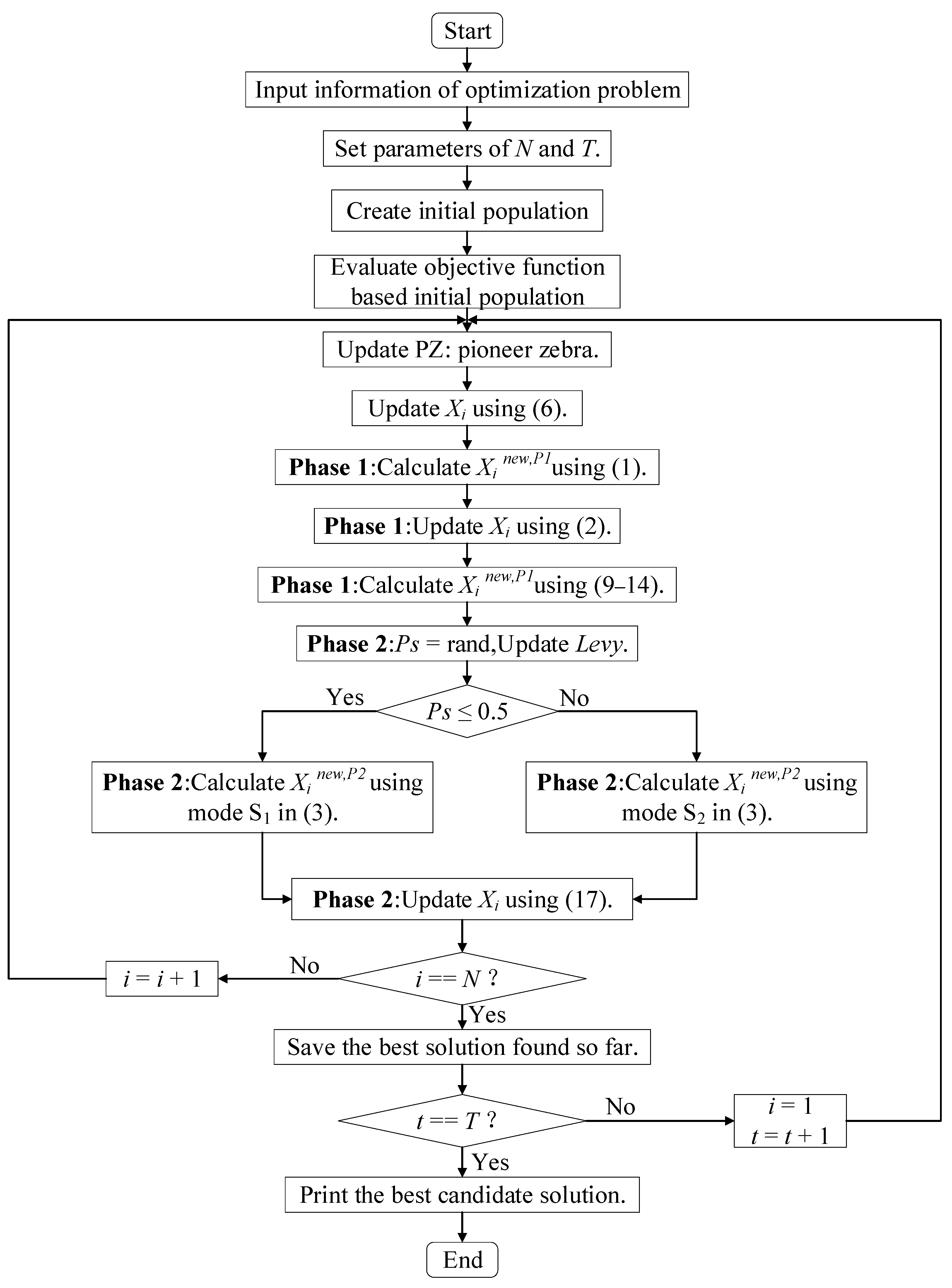
3.4. The Pseudo Code of the Proposed MZOA
| Algorithm 1: Pseudo-Code of Proposed MZOA |
| Start MZOA. 1. Input: The optimization problem information. 2. Set the number of iterations (T) and the number of zebras’ population (N). 3. Initialization of the position of zebras and evaluation of the objective function. 4. For t = 1: T 5. Update pioneer zebra (PZ). 6. Update the ith zebra using (6). 7. For i = 1: N 8. Phase 1: Foraging behavior 9. Calculate new status of the ith zebra using (1). 10. Update the ith zebra using (2). 11. Calculate new status of the ith zebra using (9–14). 12. Phase 2: Defense strategies against predators 13. Update the Ps, Levy. 14. If Ps < 0.5 15. Strategy 1: against lion (exploitation phase) 16. Calculate new status of the ith zebra using mode S1 in (3). 17. else 18. Strategy 2: against other predator (exploration phase) 19. Calculate new status of the ith zebra using mode S2 in (3). 20. end if 21. Update the ith zebra using (17). 22. end for i = 1: N 23. Save best candidate solution so far. 24. end for t = 1: T 25. Output: The best solution obtained by MZOA for given optimization problem. End MZOA. |
3.5. Algorithm Complexity Analysis
4. Simulation Experiment Analysis
4.1. Experiment and Environment Setup
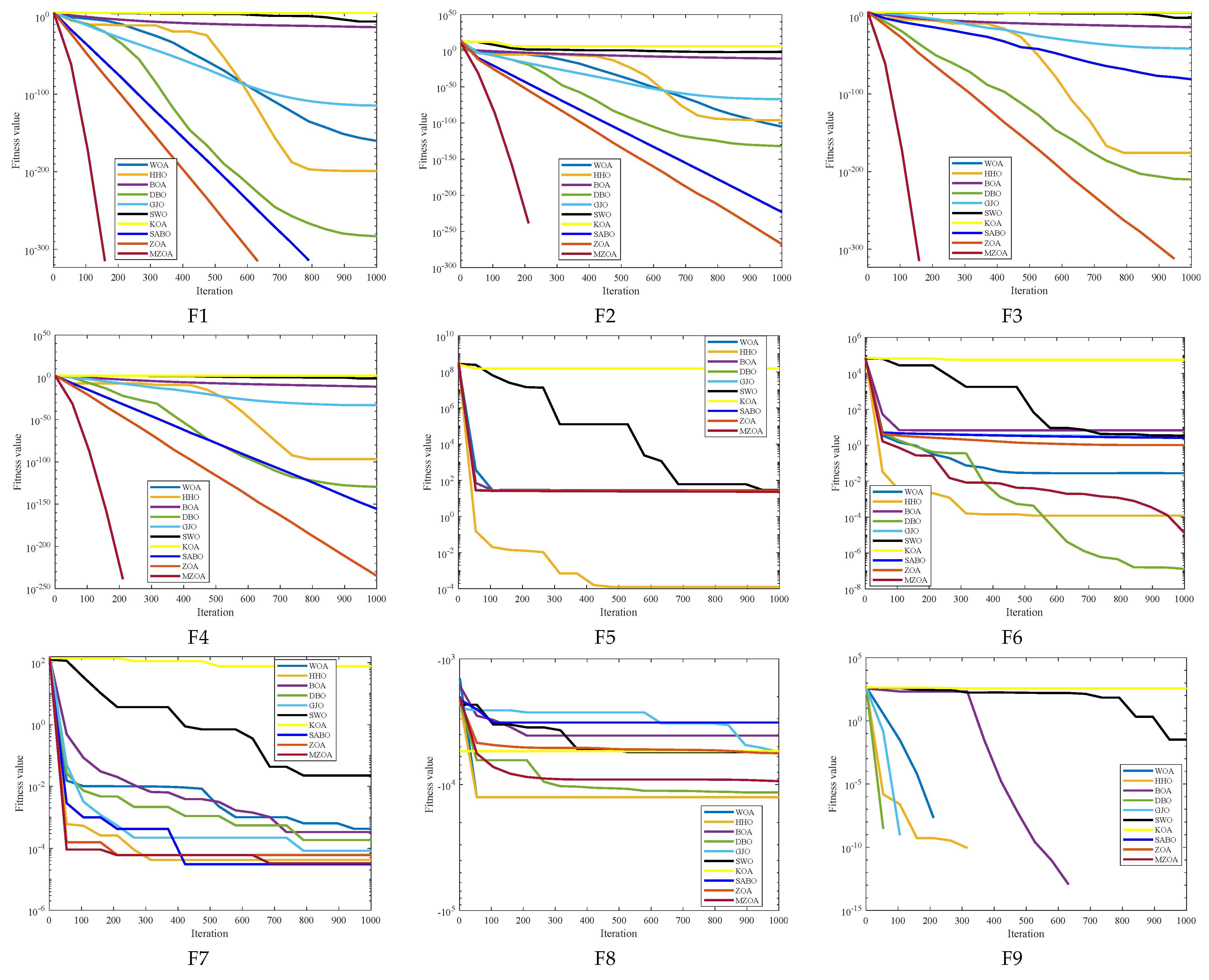
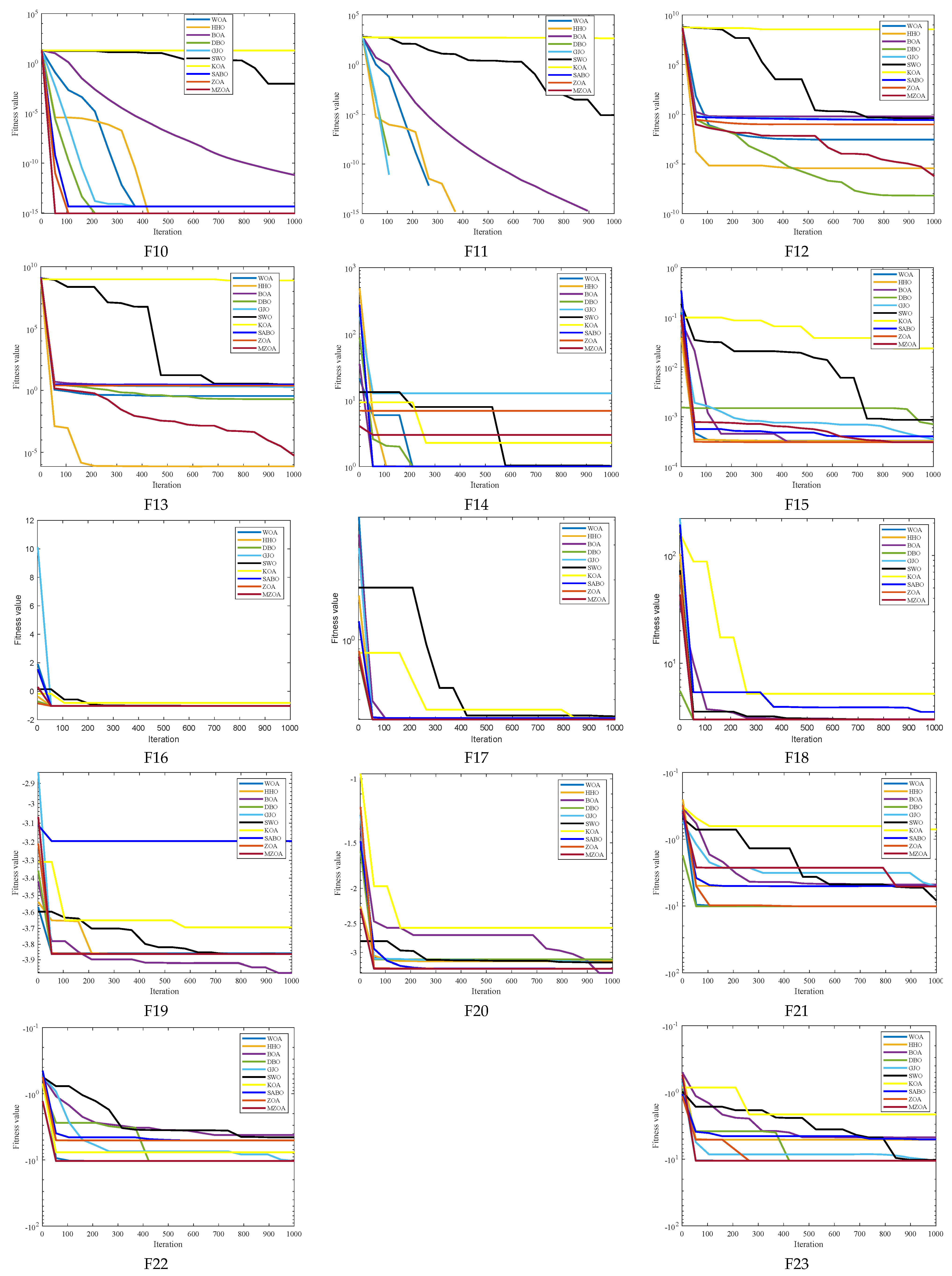
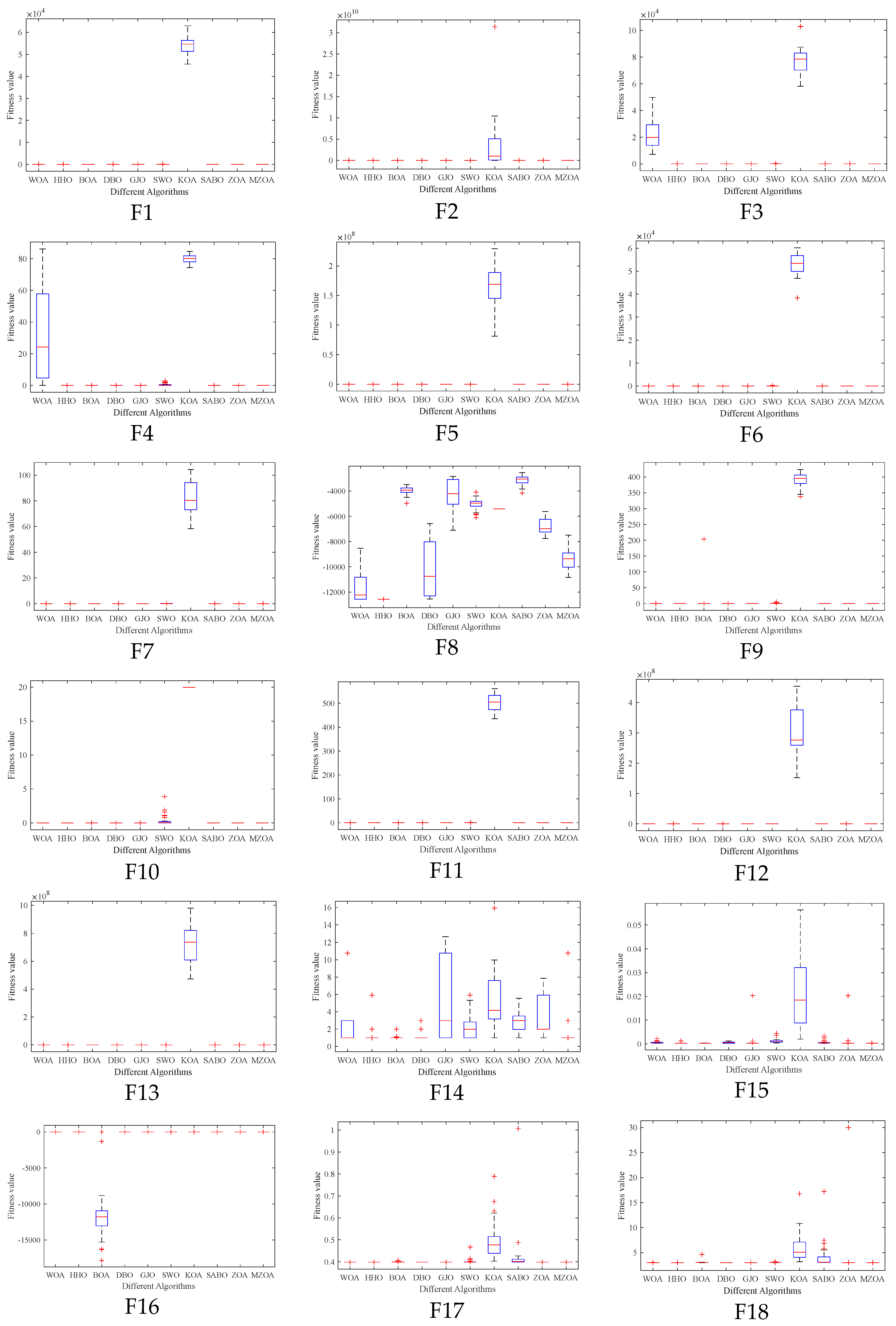
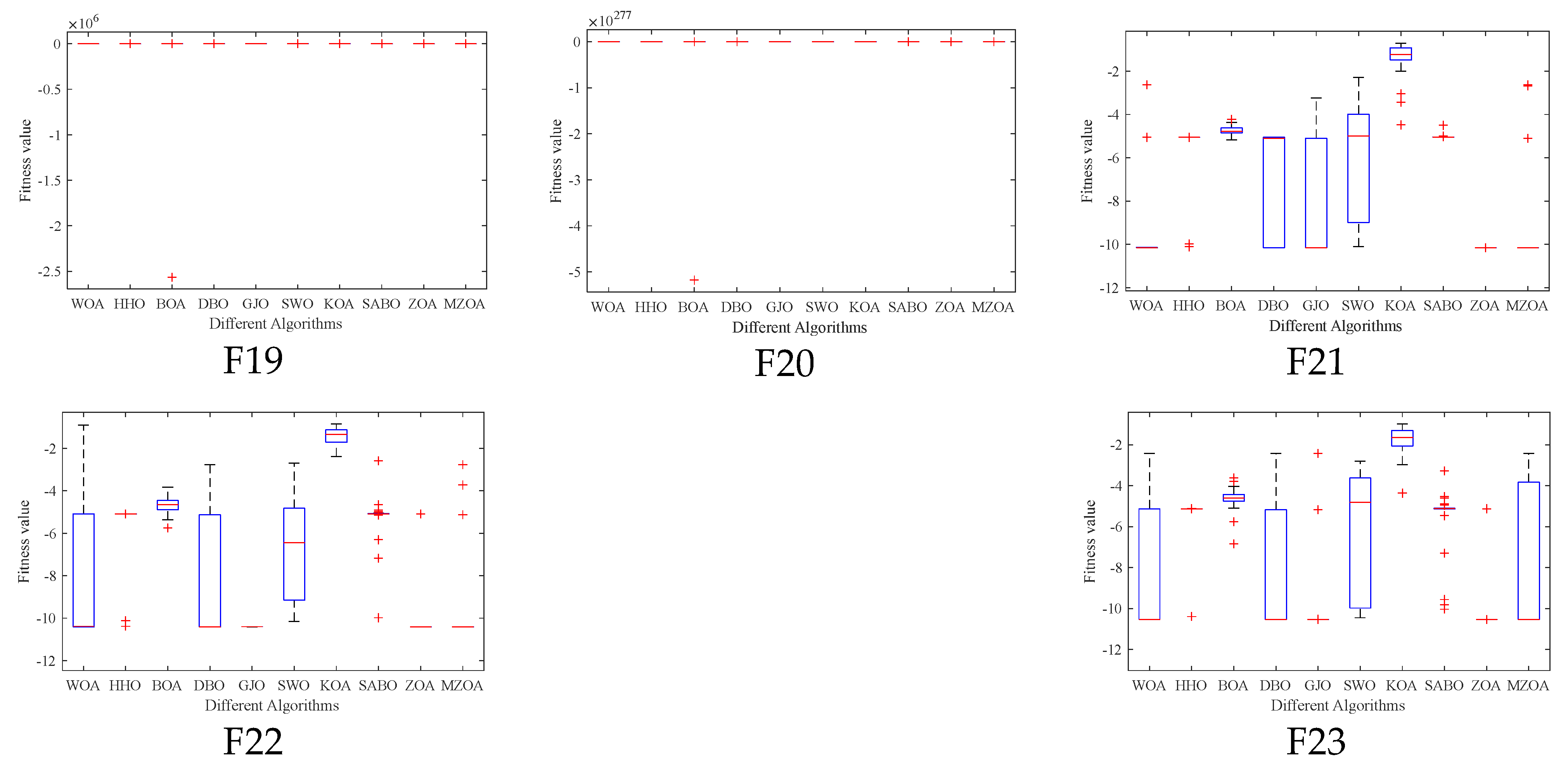
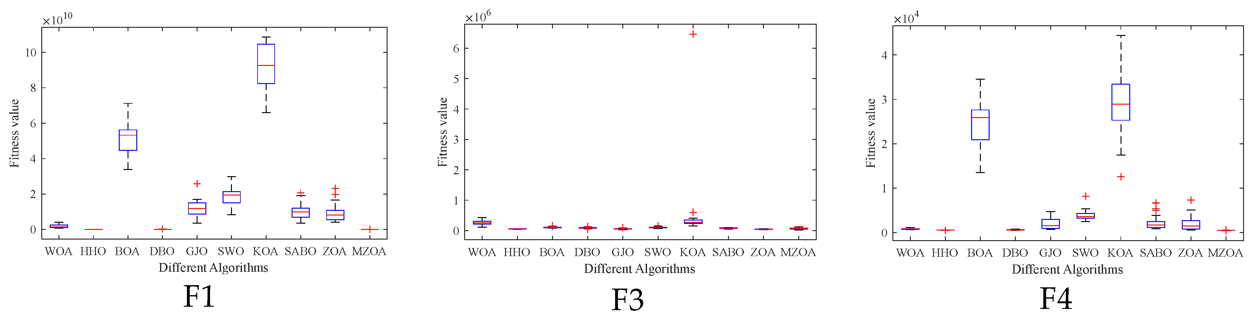
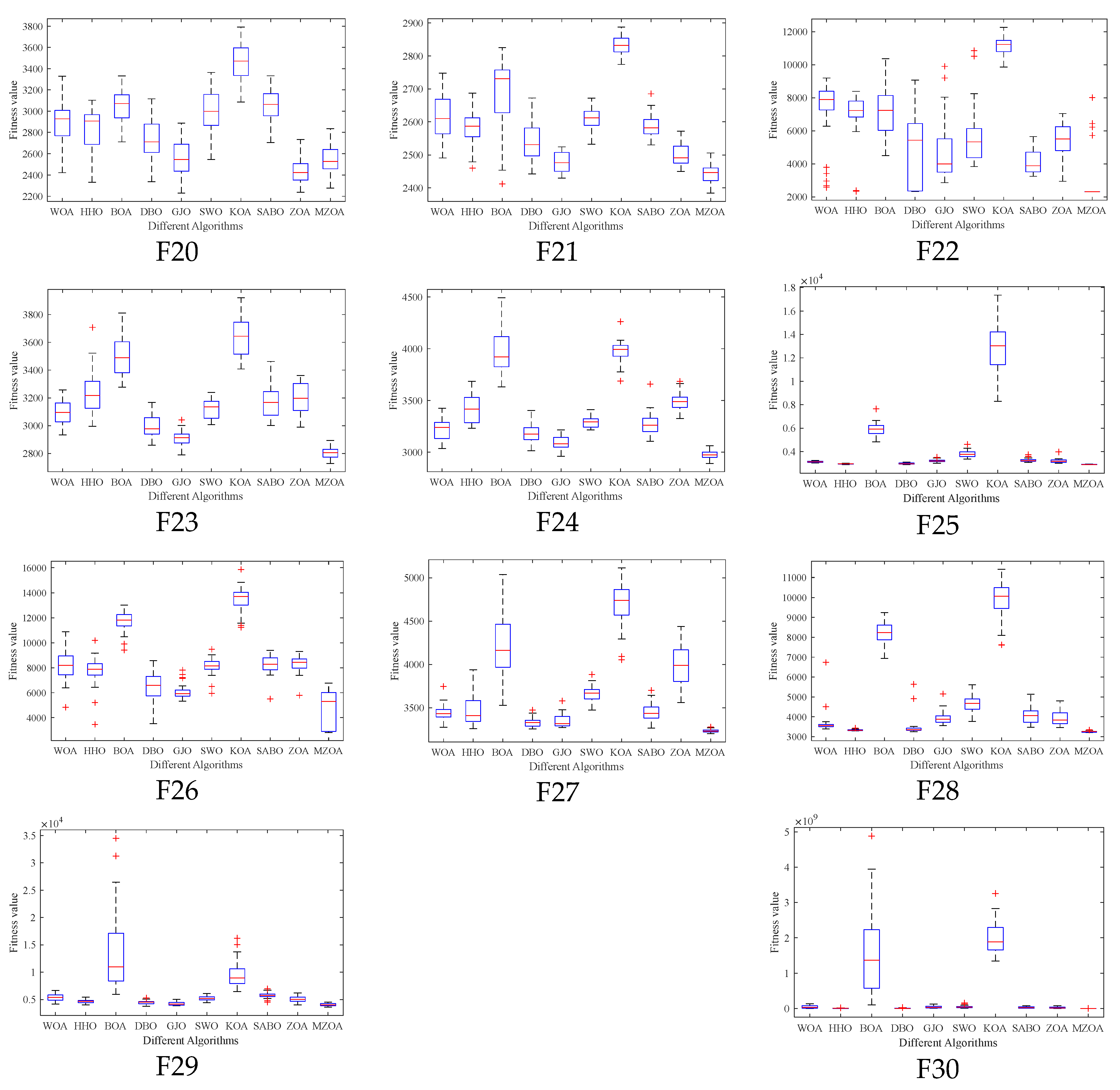
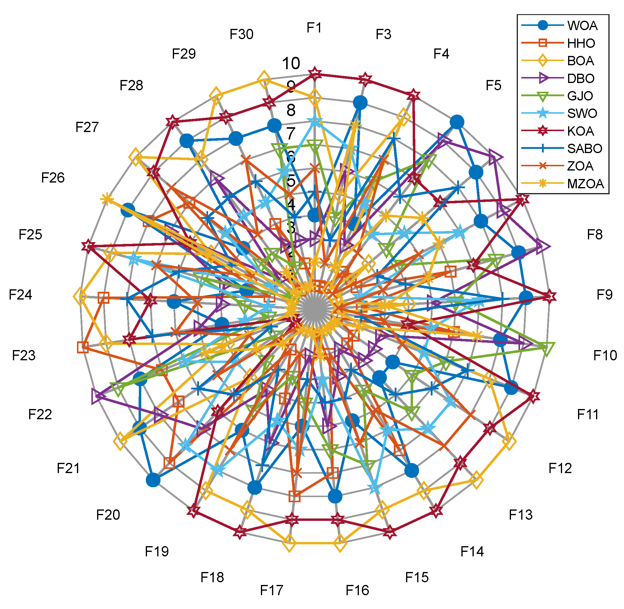
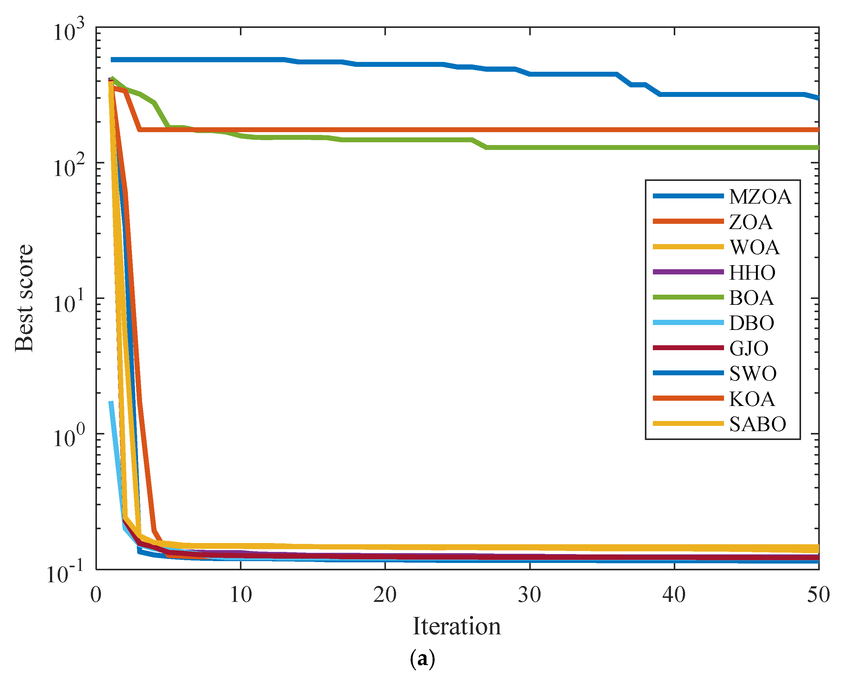
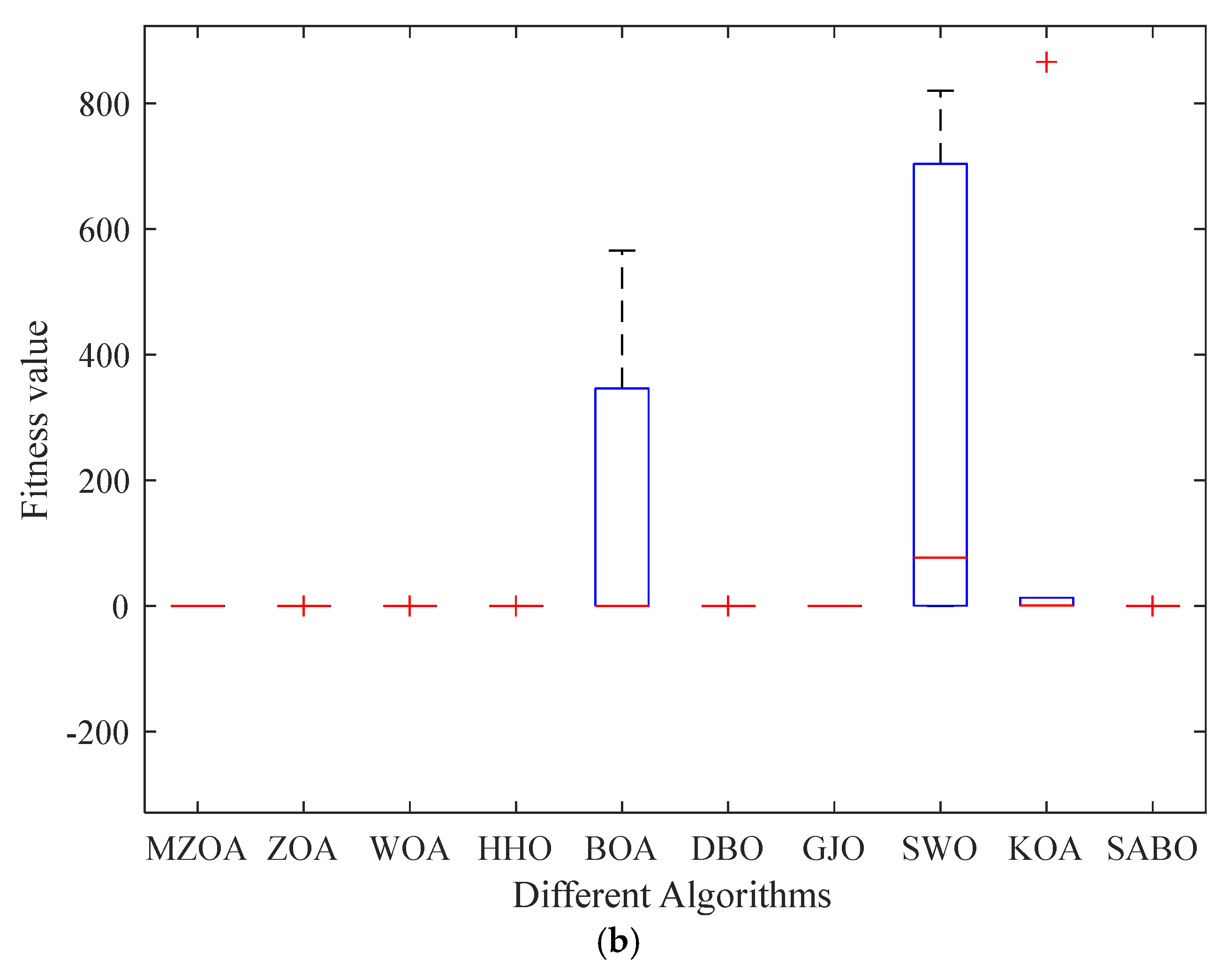
4.2. Comparative Analysis of MZOA with Other Algorithms
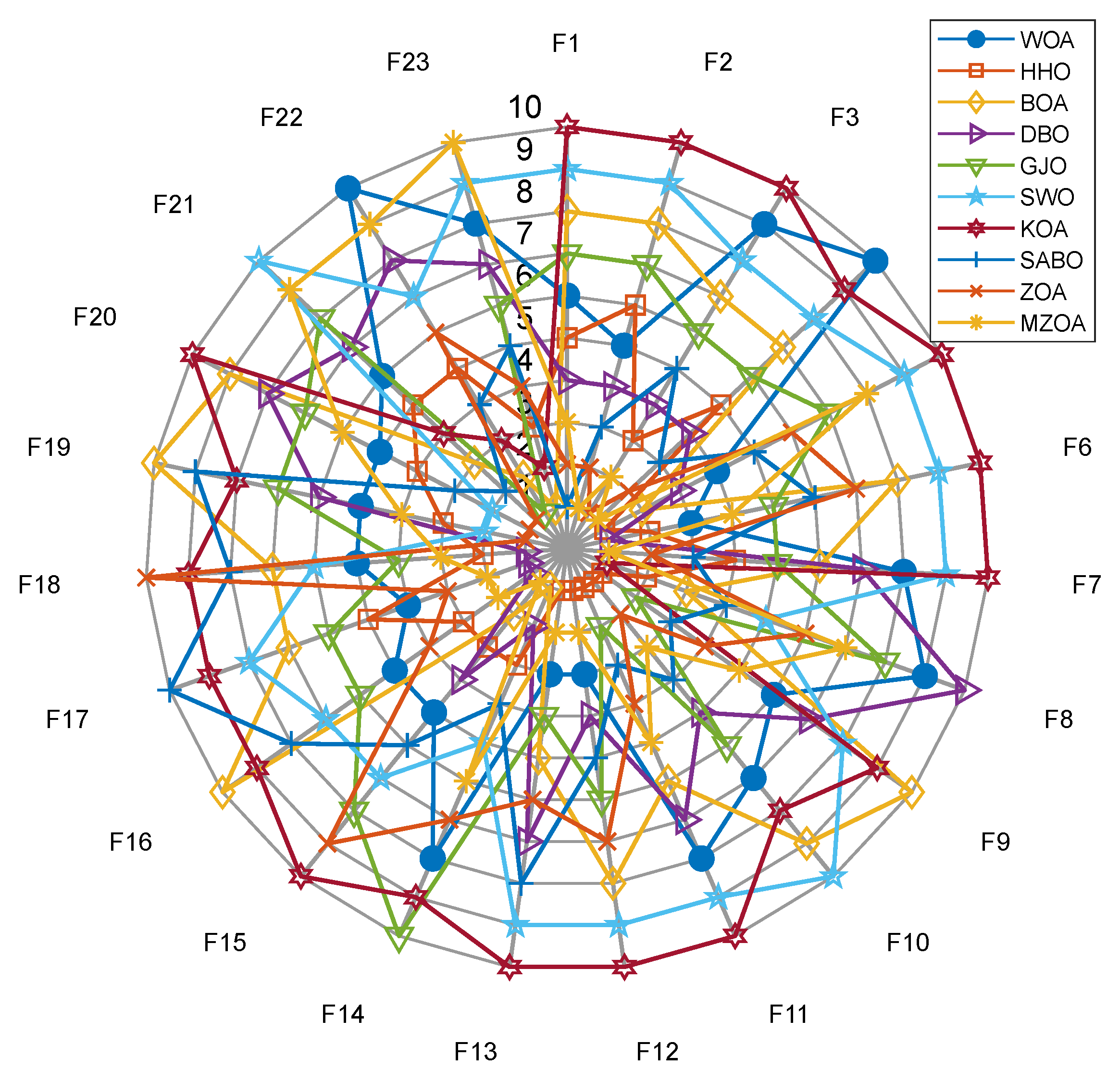
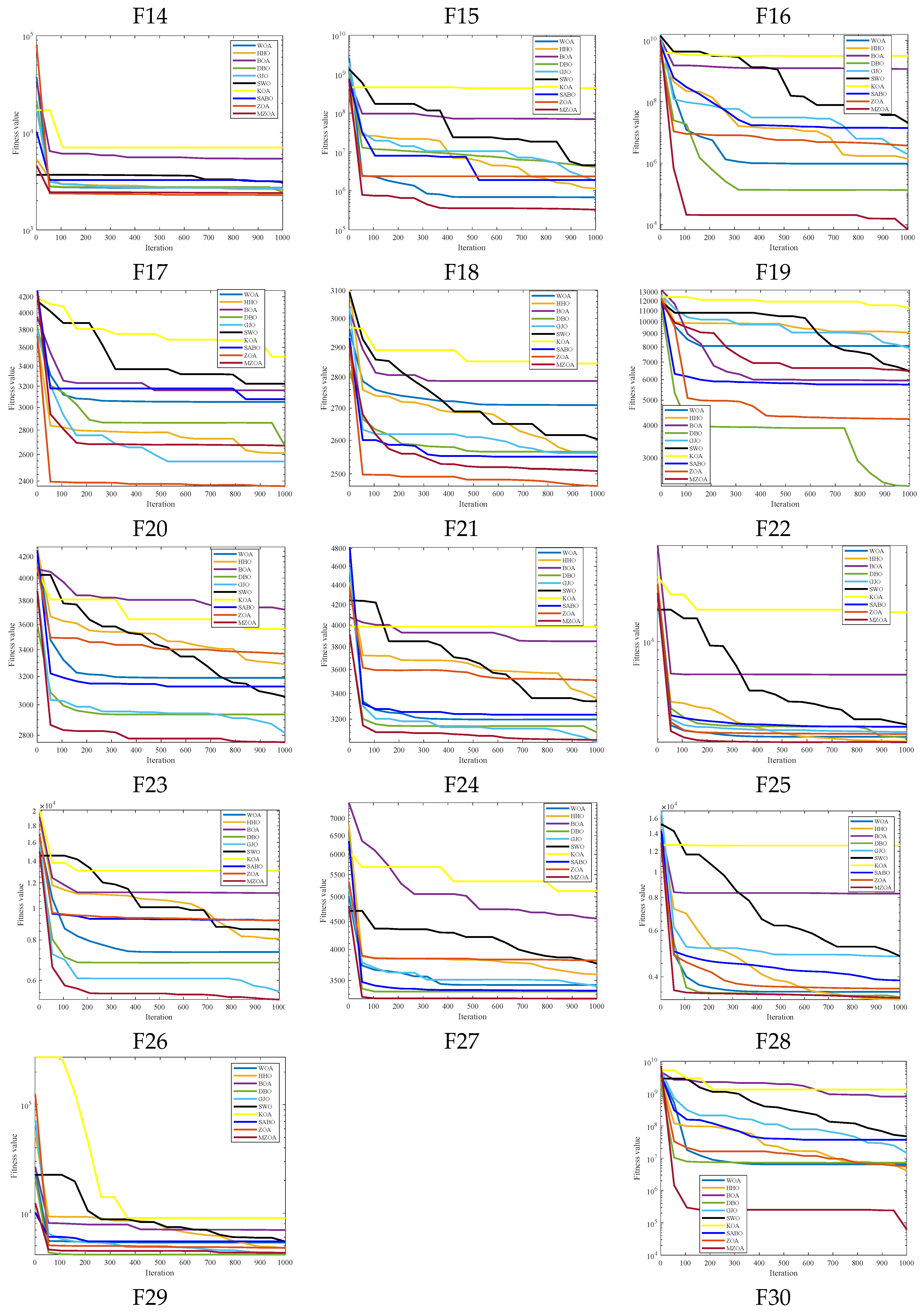
4.3. Further Comparative Experiments of the Algorithm
4.4. Engineering Design Problem
4.4.1. Tension/Compression Spring Design
4.4.2. Cantilever Beam
5. Robot Path Planning Problem
5.1. Path Planning Fitness Function
5.2. Path Planning Environment Setup
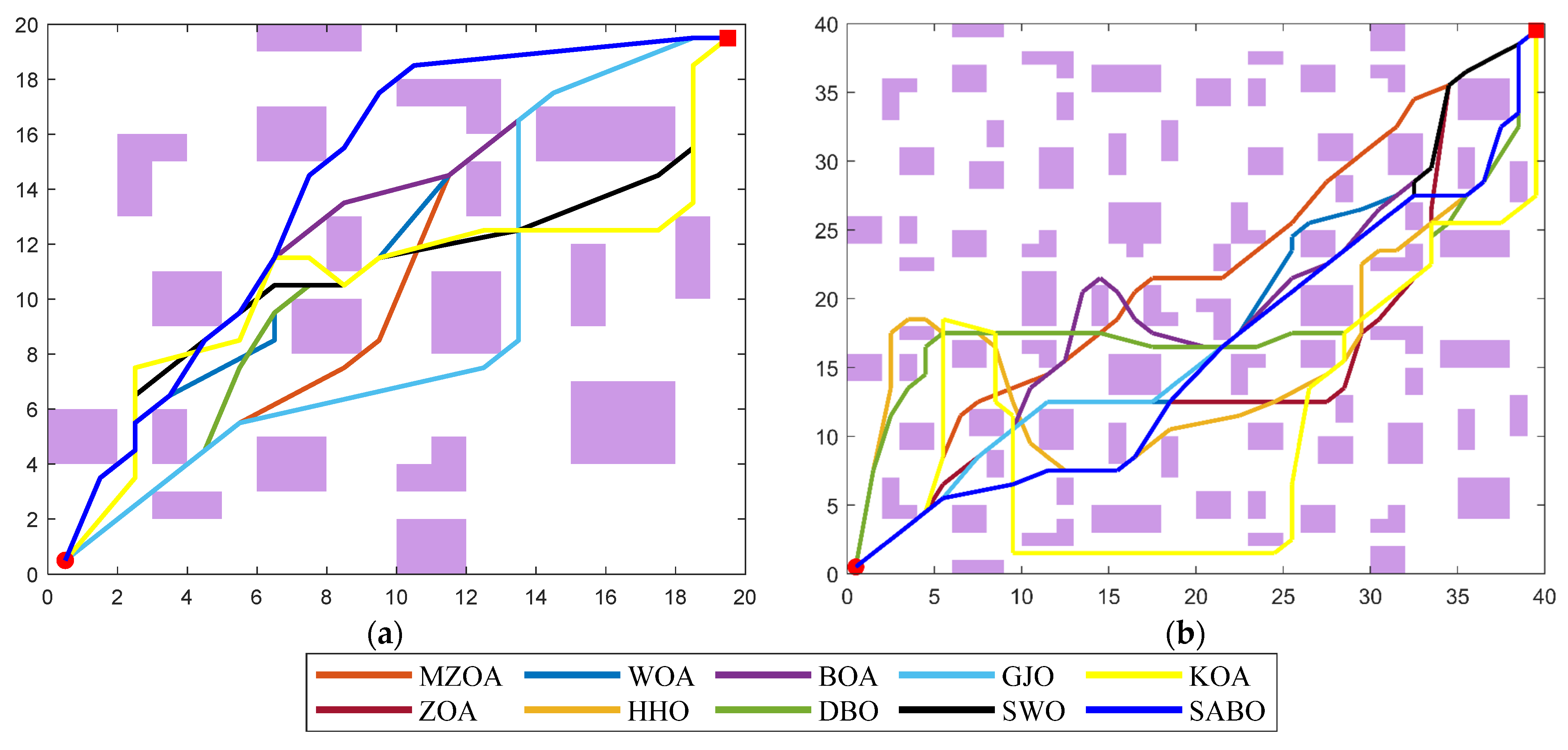
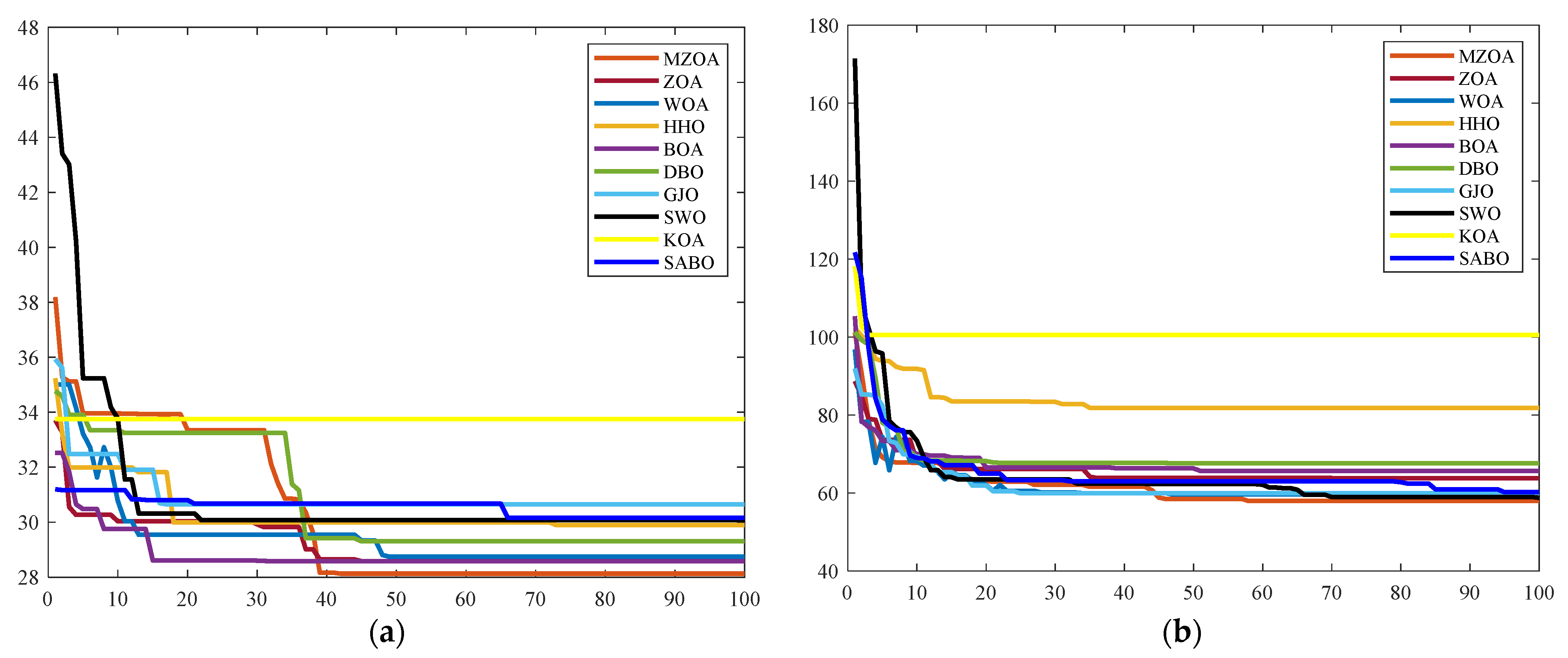
5.3. Robot Path Planning Simulation and Result Analysis
6. Conclusions
Author Contributions
Funding
Data Availability Statement
Conflicts of Interest
References
- Gharehchopogh, F.S. Quantum-inspired metaheuristic algorithms: Comprehensive survey and classification. Artif. Intell. Rev. 2023, 56, 5479–5543. [Google Scholar] [CrossRef]
- Dehghani, M.; Montazeri, Z.; Trojovská, E.; Trojovsky, P. Coati Optimization Algorithm: A new bio-inspired metaheuristic algorithm for solving optimization problems. Knowl.-Based Syst. 2023, 259, 110011. [Google Scholar] [CrossRef]
- Pan, J.S.; Zhang, L.G.; Wang, R.B.; Snášel, V.; Chu, S. Gannet optimization algorithm: A new metaheuristic algorithm for solving engineering optimization problems. Math. Comput. Simul. 2022, 202, 343–373. [Google Scholar] [CrossRef]
- Li, G.; Zhang, T.; Tsai, C.Y.; Yao, L.; Lu, Y.; Tang, J. Review of the metaheuristic algorithms in applications: Visual analysis based on bibliometrics (1994–2023). Expert Syst. Appl. 2024, 255, 124857. [Google Scholar] [CrossRef]
- Hashim, F.A.; Houssein, E.H.; Hussain, K.; Mabrouk, M.; Al-Atabany, W. Honey Badger Algorithm: New metaheuristic algorithm for solving optimization problems. Math. Comput. Simul. 2022, 192, 84–110. [Google Scholar] [CrossRef]
- Cao, L.; Chen, H.; Chen, Y.; Yue, Y.; Zhang, X. Bio-Inspired Swarm Intelligence Optimization Algorithm-Aided Hybrid TDOA/AOA-Based Localization. Biomimetics 2023, 8, 186. [Google Scholar] [CrossRef]
- Chen, C.; Cao, L.; Chen, Y.; Chen, B.; Yue, Y. A comprehensive survey of convergence analysis of beetle antennae search algorithm and its applications. Artif. Intell. Rev. 2024, 57, 141. [Google Scholar] [CrossRef]
- Yue, Y.; Cao, L.; Zhang, Y. Novel WSN Coverage Optimization Strategy Via Monarch Butterfly Algorithm and Particle Swarm Optimization. Wirel. Pers. Commun. 2024, 135, 2255–2280. [Google Scholar] [CrossRef]
- Chen, B.; Cao, L.; Chen, C.; Chen, Y.; Yue, Y. A comprehensive survey on the chicken swarm optimization algorithm and its applications: State-of-the-art and research challenges. Artif. Intell. Rev. 2024, 57, 170. [Google Scholar] [CrossRef]
- Di Caprio, D.; Ebrahimnejad, A.; Alrezaamiri, H.; Santos-Arteaga, F. A novel ant colony algorithm for solving shortest path problems with fuzzy arc weights. Alex. Eng. J. 2022, 61, 3403–3415. [Google Scholar] [CrossRef]
- Wang, S.; Cao, L.; Chen, Y.; Chen, C.; Yue, Y.; Zhu, W. Gorilla optimization algorithm combining sine cosine and cauchy variations and its engineering applications. Sci. Rep. 2024, 14, 7578. [Google Scholar] [CrossRef] [PubMed]
- Wang, Z.; Tian, J.; Feng, K. Optimal allocation of regional water resources based on simulated annealing particle swarm optimization algorithm. Energy Rep. 2022, 8, 9119–9126. [Google Scholar] [CrossRef]
- Xue, J.; Shen, B. Dung beetle optimizer: A new meta-heuristic algorithm for global optimization. J. Supercomput. 2023, 79, 7305–7336. [Google Scholar] [CrossRef]
- Yue, Y.; You, H.; Wang, S.; Cao, L. Improved whale optimization algorithm and its application in heterogeneous wireless sensor networks. Int. J. Distrib. Sens. Netw. 2021, 17, 15501477211018140. [Google Scholar] [CrossRef]
- Heidari, A.A.; Mirjalili, S.; Faris, H.; Aljarah, I.; Mafarja, M.; Chen, H. Harris hawks optimization: Algorithm and applications. Future Gener. Comput. Syst. 2019, 97, 849–872. [Google Scholar] [CrossRef]
- Yue, Y.; Cao, L.; Lu, D.; Hu, Z.; Xu, M.; Wang, S.; Li, B.; Ding, H. Review and empirical analysis of sparrow search algorithm. Artif. Intell. Rev. 2023, 56, 10867–10919. [Google Scholar] [CrossRef]
- Yue, Y.; Cao, L.; Chen, H.; Chen, Y.; Su, Z. Towards an Optimal KELM Using the PSO-BOA Optimization Strategy with Applications in Data Classification. Biomimetics 2023, 8, 306. [Google Scholar] [CrossRef]
- Hu, G.; Huang, F.; Chen, K.; Wei, G. MNEARO: A meta swarm intelligence optimization algorithm for engineering applications. Comput. Methods Appl. Mech. Eng. 2024, 419, 116664. [Google Scholar] [CrossRef]
- Zhu, F.; Li, G.; Tang, H.; Li, Y.; Lv, X.; Wang, X. Dung beetle optimization algorithm based on quantum computing and multi-strategy fusion for solving engineering problems. Expert Syst. Appl. 2024, 236, 121219. [Google Scholar] [CrossRef]
- Liu, Y.; As’arry, A.; Hassan, M.K.; Hairuddin, A.; Mohamad, H. Review of the grey wolf optimization algorithm: Variants and applications. Neural Comput. Appl. 2024, 36, 2713–2735. [Google Scholar] [CrossRef]
- Ran, X.; Suyaroj, N.; Tepsan, W.; Ma, J.; Zhu, X.; Deng, W. A hybrid genetic-fuzzy ant colony optimization algorithm for automatic K-means clustering in urban global positioning system. Eng. Appl. Artif. Intell. 2024, 137, 109237. [Google Scholar] [CrossRef]
- Trojovská, E.; Dehghani, M.; Trojovský, P. Zebra optimization algorithm: A new bio-inspired optimization algorithm for solving optimization algorithm. IEEE Access 2022, 10, 49445–49473. [Google Scholar] [CrossRef]
- Mohapatra, S.; Mohapatra, P. American zebra optimization algorithm for global optimization problems. Sci. Rep. 2023, 13, 5211. [Google Scholar] [CrossRef] [PubMed]
- Elymany, M.M.; Enany, M.A.; Elsonbaty, N.A. Hybrid optimized-ANFIS based MPPT for hybrid microgrid using zebra optimization algorithm and artificial gorilla troops optimizer. Energy Convers. Manag. 2024, 299, 117809. [Google Scholar] [CrossRef]
- Bui, N.D.H.; Duong, T.L. An Improved Zebra Optimization Algorithm for Solving Transmission Expansion Planning Problem with Penetration of Renewable Energy Sources. Int. J. Intell. Eng. Syst. 2024, 17, 202–211. [Google Scholar]
- Aydemir, S.B.; Onay, F.K.; Yalcin, E. Empowered chaotic local search-based differential evolution algorithm with entropy-based hybrid objective function for brain tumor segmentation. Biomed. Signal Process. Control 2024, 96, 106631. [Google Scholar] [CrossRef]
- Qi, Z.; Peng, S.; Wu, P.; Tseng, M. Renewable Energy Distributed Energy System Optimal Configuration and Performance Analysis: Improved Zebra Optimization Algorithm. Sustainability 2024, 16, 5016. [Google Scholar] [CrossRef]
- Amin, R.; El-Taweel, G.; Ali, A.F.; Tahoun, M. Hybrid Chaotic Zebra Optimization Algorithm and Long Short-Term Memory for Cyber Threats Detection. IEEE Access 2024, 12, 93235–93260. [Google Scholar] [CrossRef]
- Krithiga, G.; Senthilkumar, S.; Alharbi, M.; Mangaiyarkarasi, S.P. Design of modified long short-term memory-based zebra optimization algorithm for limiting the issue of SHEPWM in multi-level inverter. Sci. Rep. 2024, 14, 22439. [Google Scholar] [CrossRef]
- Dama, A.; Khalaf, O.I.; Chandra, G.R. Enhancing the Zebra Optimization Algorithm with Chaotic Sinusoidal Map for Versatile Optimization. Iraqi J. Comput. Sci. Math. 2024, 5, 307–319. [Google Scholar]
- El-Hageen, H.M.; Alfaifi, Y.H.; Albalawi, H.; Alzahmi, A.; Alatwi, A.M.; Ali, A.F.; Mead, M.A. Chaotic zebra optimization algorithm for increasing the lifetime of wireless sensor network. J. Netw. Syst. Manag. 2024, 32, 85. [Google Scholar] [CrossRef]
- Abdelmalek, F.; Afghoul, H.; Krim, F.; Zabia, D.E.; Trabelsi, H.; Bajaj, M.; Blazek, V. Experimental validation of effective zebra optimization algorithm-based MPPT under partial shading conditions in photovoltaic systems. Sci. Rep. 2024, 14, 26047. [Google Scholar] [CrossRef] [PubMed]
- Khadanga, R.K.; Das, D.; Panda, S. Design and Analysis of SSSC--Based Damping Controller: A Novel Modified Zebra Optimization Algorithm Approach. J. Electr. Comput. Eng. 2024, 2024, 4590764. [Google Scholar] [CrossRef]
- Yang, B.; Liu, Y.; Liu, Z.; Zhu, Q.; Li, D. Classification of Rock Mass Quality in Underground Rock Engineering with Incomplete Data Using XGBoost Model and Zebra Optimization Algorithm. Appl. Sci. 2024, 14, 7074. [Google Scholar] [CrossRef]
- Song, H.; Zhang, M.; Shi, Q. Capacity Optimization of Hybrid Energy Storage System Based on Improved Zebra Optimization Algorithm. In Proceedings of the 2024 IEEE 7th Information Technology, Networking, Electronic and Automation Control Conference (ITNEC), Chongqing, China, 20–22 September 2024; IEEE: New York, NY, USA, 2024; Volume 7, pp. 1390–1394. [Google Scholar]
- Janakiraman, S.; Deva Priya, M.; Karthick, S. American Zebra Optimization Algorithm-based Clustering Protocol for Reliable Data Routing in Internet of Things. In Proceedings of International Conference on Recent Trends in Computing; Springer Nature: Singapore, 2023; pp. 779–794. [Google Scholar]
- Ouyang, C.; Zhu, D.; Qiu, Y. Lens learning sparrow search algorithm. Math. Probl. Eng. 2021, 2021, 9935090. [Google Scholar] [CrossRef]
- Yuan, P.; Zhang, T.; Yao, L.; Lu, Y.; Zhuang, W. A hybrid golden jackal optimization and golden sine algorithm with dynamic lens-imaging learning for global optimization problems. Appl. Sci. 2022, 12, 9709. [Google Scholar] [CrossRef]
- Ai, C.; He, S.; Fan, X. Parameter estimation of fractional-order chaotic power system based on lens imaging learning strategy state transition algorithm. IEEE Access 2023, 11, 13724–13737. [Google Scholar] [CrossRef]
- Wu, X.; Li, J.; Zhou, G.; Lu, B.; Li, Q.; Yang, H. RRG-GAN restoring network for simple lens imaging system. Sensors 2021, 21, 3317. [Google Scholar] [CrossRef]
- Zhang, J.; Zhang, G.; Kong, M.; Zhang, T. Adaptive infinite impulse response system identification using an enhanced golden jackal optimization. J. Supercomput. 2023, 79, 10823–10848. [Google Scholar] [CrossRef]
- Liu, S. Triangular Walking Strategy Based Sand Cat Swarm Optimization for Color Level Determination in Visual Communication. In Proceedings of the 2024 International Conference on Intelligent Algorithms for Computational Intelligence Systems (IACIS), Atlantic Beach, FL, USA, 2–5 October 2024; IEEE: New York, NY, USA, 2024; pp. 1–5. [Google Scholar]
- Hong, Y.N.G.; Jeong, J.; Kim, P.; Shin, C. Lower extremity biomechanics while walking on a triangle-shaped slope. Trans. Korean Soc. Mech. Eng. B 2017, 41, 153–160. [Google Scholar]
- Chawla, M.; Duhan, M. Levy flights in metaheuristics optimization algorithms—A review. Appl. Artif. Intell. 2018, 32, 802–821. [Google Scholar] [CrossRef]
- Kaidi, W.; Khishe, M.; Mohammadi, M. Dynamic levy flight chimp optimization. Knowl.-Based Syst. 2022, 235, 107625. [Google Scholar] [CrossRef]
- Dhawale, P.G.; Kamboj, V.K.; Bath, S.K. A levy flight based strategy to improve the exploitation capability of arithmetic optimization algorithm for engineering global optimization problems. Trans. Emerg. Telecommun. Technol. 2023, 34, e4739. [Google Scholar] [CrossRef]
- Li, J.; An, Q.; Lei, H.; Deng, Q.; Wang, G. Survey of Levy flight-based metaheuristics for optimization. Mathematics 2022, 10, 2785. [Google Scholar] [CrossRef]
- Wang, Z.; Chen, Y.; Ding, S.; Liang, D.; He, H. A novel particle swarm optimization algorithm with Levy flight and orthogonal learning. Swarm Evol. Comput. 2022, 75, 101207. [Google Scholar] [CrossRef]
- Chen, Y.; Xi, J.; Wang, H.; Liu, X. Grey wolf optimization algorithm based on dynamically adjusting inertial weight and levy flight strategy. Evol. Intell. 2023, 16, 917–927. [Google Scholar] [CrossRef]
- Cui, Y.; Shi, R.; Dong, J. CLTSA: A novel tunicate swarm algorithm based on chaotic-Levy flight strategy for solving optimization problems. Mathematics 2022, 10, 3405. [Google Scholar] [CrossRef]
- Mao, X.; Song, S.; Ding, F. Optimal BP neural network algorithm for state of charge estimation of lithium-ion battery using PSO with Levy flight. J. Energy Storage 2022, 49, 104139. [Google Scholar] [CrossRef]
- Wang, W.; Tian, J. An improved nonlinear tuna swarm optimization algorithm based on circle chaos map and levy flight operator. Electronics 2022, 11, 3678. [Google Scholar] [CrossRef]
- Gharehchopogh, F.S.; Gholizadeh, H. A comprehensive survey: Whale Optimization Algorithm and its applications. Swarm Evol. Comput. 2019, 48, 1–24. [Google Scholar] [CrossRef]
- Alabool, H.M.; Alarabiat, D.; Abualigah, L.; Heidari, A. Harris hawks optimization: A comprehensive review of recent variants and applications. Neural Comput. Appl. 2021, 33, 8939–8980. [Google Scholar] [CrossRef]
- Arora, S.; Singh, S. Butterfly optimization algorithm: A novel approach for global optimization. Soft Comput. 2019, 23, 715–734. [Google Scholar] [CrossRef]
- Shen, Q.; Zhang, D.; Xie, M.; He, Q. Multi-strategy enhanced dung beetle optimizer and its application in three-dimensional UAV path planning. Symmetry 2023, 15, 1432. [Google Scholar] [CrossRef]
- Houssein, E.H.; Abdelkareem, D.A.; Emam, M.M.; Hameed, M.A.; Younan, M. An efficient image segmentation method for skin cancer imaging using improved golden jackal optimization algorithm. Comput. Biol. Med. 2022, 149, 106075. [Google Scholar] [CrossRef]
- Abdel-Basset, M.; Mohamed, R.; Jameel, M.; Abouhawwash, M. Spider wasp optimizer: A novel meta-heuristic optimization algorithm. Artif. Intell. Rev. 2023, 56, 11675–11738. [Google Scholar] [CrossRef]
- Abdel-Basset, M.; Mohamed, R.; Azeem, S.A.A.; Jameel, M.; Abouhawwash, M. Kepler optimization algorithm: A new metaheuristic algorithm inspired by Kepler’s laws of planetary motion. Knowl.-Based Syst. 2023, 268, 110454. [Google Scholar] [CrossRef]
- Trojovský, P.; Dehghani, M. Subtraction-average-based optimizer: A new swarm-inspired metaheuristic algorithm for solving optimization problems. Biomimetics 2023, 8, 149. [Google Scholar] [CrossRef]
- Shareef, S.K.K.; Chaitanya, R.K.; Chennupalli, S.; Chokkakula, D.; Kiran, K.V.D.; Pamula, U.; Vatambeti, R. Enhanced botnet detection in IoT networks using zebra optimization and dual-channel GAN classification. Sci. Rep. 2024, 14, 17148. [Google Scholar] [CrossRef]


| No. | Functions | Fi = Fi(x) | |
|---|---|---|---|
| F1 | Sphere Function | 0 | |
| F2 | Schwefel’s Problem 2.22 | 0 | |
| Unimodal | F3 | Schwefel’s Problem 1.2 | 0 |
| Functions | F4 | Schwefel’s Problem 2.21 | 0 |
| F5 | Generalized Rosenbrock’s Function | 0 | |
| F6 | Step Function | 0 | |
| F7 | Quartic Function, i.e., Noise | 0 | |
| F8 | Generalized Schwefel’s Problem 2.26 | −12,569.5 | |
| Simple | F9 | Generalized Rastrigin’s Function | 0 |
| Multimodal | F10 | Ackley’s Function | 0 |
| Functions | F11 | Generalized Griewank’s Function | 0 |
| F12 | Generalized Penalized Function 1 | 0 | |
| F13 | Generalized Penalized Function 2 | 0 | |
| F14 | Shekel’s Foxholes Function | 0.9980 | |
| F15 | Kowalik’s Function | 0.0003075 | |
| F16 | Six-Hump Camel-Back Function | −1.0316 | |
| F17 | Branin Function | 0.3979 | |
| Composition | F18 | Goldstein-Price Function | 2.99999999 |
| Functions | F19 | Hartman’s Family | −3.8628 |
| F20 | Hartman’s Family | −3.3220 | |
| F21 | Shekel’s Family | −10.1532 | |
| F22 | Shekel’s Family | −10.4029 | |
| F23 | Shekel’s Family | −10.5363 |
| No. | Functions | Fi = Fi(x) | |
|---|---|---|---|
| Unimodal Functions | 1 | Shifted and Rotated Bent Cigar Function | 100 |
| 2 | Shifted and Rotated Sum of Different Power Function | 200 | |
| 3 | Shifted and Rotated Zakharov Function | 300 | |
| Simple Multimodal Functions | 4 | Shifted and Rotated Rosenbrock’s Function | 400 |
| 5 | Shifted and Rotated Rastrigin’s Function | 500 | |
| 6 | Shifted and Rotated Expanded Scaffer’s F6 Function | 600 | |
| 7 | Shifted and Rotated Lunacek Bi_Rastrigin Function | 700 | |
| 8 | Shifted and Rotated Non-Continuous Rastrigin’s Function | 800 | |
| 9 | Shifted and Rotated Levy Function | 900 | |
| 10 | Shifted and Rotated Schwefel’s Function | 1000 | |
| Hybrid Functions | 11 | Hybrid Function 1 (N = 3) | 1100 |
| 12 | Hybrid Function 2 (N = 3) | 1200 | |
| 13 | Hybrid Function 3 (N = 3) | 1300 | |
| 14 | Hybrid Function 4 (N = 4) | 1400 | |
| 15 | Hybrid Function 5 (N = 4) | 1500 | |
| 16 | Hybrid Function 6 (N = 4) | 1600 | |
| 17 | Hybrid Function 6 (N = 5) | 1700 | |
| 18 | Hybrid Function 6 (N = 5) | 1800 | |
| 19 | Hybrid Function 6 (N = 5) | 1900 | |
| 20 | Hybrid Function 6 (N = 6) | 2000 | |
| Composition Functions | 21 | Composition Function 1 (N = 3) | 2100 |
| 22 | Composition Function 2 (N = 3) | 2200 | |
| 23 | Composition Function 3 (N = 4) | 2300 | |
| 24 | Composition Function 4 (N = 4) | 2400 | |
| 25 | Composition Function 5 (N = 5) | 2500 | |
| 26 | Composition Function 6 (N = 5) | 2600 | |
| 27 | Composition Function 7 (N = 6) | 2700 | |
| 28 | Composition Function 8 (N = 6) | 2800 | |
| 29 | Composition Function 9 (N = 3) | 2900 | |
| 30 | Composition Function 10 (N = 3) | 3000 | |
| Search Range: [−100,100] | |||
| WOA | HHO | BOA | DBO | GJO | SWO | KOA | SABO | ZOA | MZOA | ||
|---|---|---|---|---|---|---|---|---|---|---|---|
| F1 | min | 3.74 × 10−166 | 5.31 × 10−209 | 1.57 × 10⁻¹⁴ | 5.65 × 10−307 | 6.38 × 10−119 | 1.18 × 10⁻⁸ | 4.56 × 10+4 | 0.00 × 10+0 | 0.00 × 10+0 | 0.00 × 10+0 |
| F1 | std | 4.28 × 10−150 | 0.00 × 10+0 | 9.64 × 10⁻¹⁶ | 0.00 × 10+0 | 3.22 × 10−111 | 7.66 × 10+0 | 4.58 × 10+3 | 0.00 × 10+0 | 0.00 × 10+0 | 0.00 × 10+0 |
| F1 | avg | 1.46 × 10−150 | 9.25 × 10−187 | 1.77 × 10⁻¹⁴ | 3.23 × 10−240 | 9.06 × 10−112 | 1.68 × 10+0 | 5.39 × 10+4 | 0.00 × 10+0 | 0.00 × 10+0 | 0.00 × 10+0 |
| F2 | min | 1.12 × 10−116 | 1.39 × 10−111 | 1.52 × 10⁻¹² | 1.98 × 10−161 | 7.41 × 10−68 | 3.49 × 10⁻⁶ | 2.35 × 10+2 | 1.36 × 10−226 | 1.82 × 10−272 | 0.00 × 10+0 |
| F2 | std | 1.13 × 10−103 | 7.55 × 10−94 | 2.73 × 10⁻¹² | 1.92 × 10−120 | 9.70 × 10−66 | 3.76 × 10⁻¹ | 6.10 × 10+9 | 0.00 × 10+0 | 0.00 × 10+0 | 0.00 × 10+0 |
| F2 | avg | 2.35 × 10−104 | 1.38 × 10−94 | 1.01 × 10⁻¹¹ | 3.50 × 10−121 | 4.84 × 10−66 | 1.49 × 10⁻¹ | 3.25 × 10+9 | 8.78 × 10−224 | 6.47 × 10−266 | 0.00 × 10+0 |
| F3 | min | 7.09 × 10+3 | 2.75 × 10−187 | 1.58 × 10⁻¹⁴ | 2.47 × 10−275 | 4.97 × 10−49 | 2.45 × 10⁻⁶ | 5.82 × 10+4 | 3.31 × 10−167 | 0.00 × 10+0 | 0.00 × 10+0 |
| F3 | std | 1.03 × 10+4 | 6.20 × 10−130 | 1.04 × 10⁻¹⁵ | 2.83 × 10−115 | 9.89 × 10−37 | 5.18 × 10+1 | 1.03 × 10+4 | 6.75 × 10−38 | 0.00 × 10+0 | 0.00 × 10+0 |
| F3 | avg | 2.18 × 10+4 | 1.13 × 10−130 | 1.80 × 10⁻¹⁴ | 5.17 × 10−116 | 2.18 × 10−37 | 1.68 × 10+1 | 7.79 × 10+4 | 1.23 × 10−38 | 0.00 × 10+0 | 0.00 × 10+0 |
| F4 | min | 5.29 × 10⁻² | 1.20 × 10−103 | 1.03 × 10⁻¹¹ | 1.71 × 10−148 | 3.62 × 10−36 | 6.49 × 10⁻⁴ | 7.44 × 10+1 | 6.22 × 10−159 | 6.76 × 10−238 | 0.00 × 10+0 |
| F4 | std | 2.93 × 10+1 | 6.83 × 10−92 | 7.58 × 10⁻¹³ | 4.58 × 10−99 | 6.04 × 10⁻³² | 7.76 × 10⁻¹ | 2.58 × 10+0 | 1.09 × 10−155 | 0.00 × 10+0 | 0.00 × 10+0 |
| F4 | avg | 3.30 × 10+1 | 1.60 × 10−92 | 1.20 × 10⁻¹¹ | 8.37 × 10−100 | 1.46 × 10⁻³² | 4.77 × 10⁻¹ | 7.99 × 10+1 | 6.50 × 10−156 | 3.32 × 10−231 | 0.00 × 10+0 |
| F5 | min | 2.62 × 10+1 | 1.34 × 10⁻⁵ | 2.88 × 10+1 | 2.46 × 10+1 | 2.62 × 10+1 | 2.89 × 10+1 | 8.14 × 10+7 | 2.70 × 10+1 | 2.68 × 10+1 | 2.28 × 10+1 |
| F5 | std | 5.38 × 10⁻¹ | 4.61 × 10⁻³ | 2.78 × 10⁻² | 1.43 × 10⁻¹ | 7.65 × 10⁻¹ | 7.49 × 10+2 | 3.42 × 10+7 | 6.41 × 10⁻¹ | 7.65 × 10⁻¹ | 1.24 × 10+0 |
| F5 | avg | 2.72 × 10+1 | 3.75 × 10⁻³ | 2.89 × 10+1 | 2.49 × 10+1 | 2.74 × 10+1 | 1.87 × 10+2 | 1.64 × 10+8 | 2.80 × 10+1 | 2.79 × 10+1 | 2.46 × 10+1 |
| F6 | min | 1.21 × 10⁻² | 1.49 × 10⁻⁶ | 3.47 × 10+0 | 5.69 × 10⁻¹² | 1.75 × 10+0 | 2.99 × 10+0 | 3.83 × 10+4 | 1.11 × 10+0 | 1.21 × 10+0 | 8.84 × 10⁻⁶ |
| F6 | std | 1.41 × 10⁻¹ | 4.80 × 10⁻⁵ | 6.75 × 10⁻¹ | 2.91 × 10⁻⁷ | 4.41 × 10⁻¹ | 4.50 × 10+1 | 4.79 × 10+3 | 5.02 × 10⁻¹ | 5.98 × 10⁻¹ | 1.55 × 10⁻¹ |
| F6 | avg | 1.01 × 10⁻¹ | 3.48 × 10⁻⁵ | 5.83 × 10+0 | 5.62 × 10⁻⁸ | 2.68 × 10+0 | 1.52 × 10+1 | 5.29 × 10+4 | 2.04 × 10+0 | 2.30 × 10+0 | 8.57 × 10⁻² |
| F7 | min | 1.24 × 10⁻⁵ | 4.70 × 10⁻⁶ | 2.11 × 10⁻⁴ | 3.51 × 10⁻⁵ | 2.79 × 10⁻⁵ | 1.55 × 10⁻³ | 5.83 × 10+1 | 4.56 × 10⁻⁷ | 1.04 × 10⁻⁵ | 4.08 × 10⁻⁹ |
| F7 | std | 2.33 × 10⁻³ | 6.28 × 10⁻⁵ | 2.67 × 10⁻⁴ | 4.83 × 10⁻⁴ | 1.40 × 10⁻⁴ | 1.53 × 10⁻² | 1.32 × 10+1 | 5.74 × 10⁻⁵ | 3.28 × 10⁻⁵ | 1.85 × 10⁻⁵ |
| F7 | avg | 1.62 × 10⁻³ | 7.52 × 10⁻⁵ | 6.44 × 10⁻⁴ | 5.95 × 10⁻⁴ | 1.77 × 10⁻⁴ | 1.92 × 10⁻² | 8.16 × 10+1 | 5.89 × 10⁻⁵ | 5.44 × 10⁻⁵ | 1.76 × 10⁻⁵ |
| F8 | min | −1.26 × 10+4 | −1.26 × 10+4 | −3.50 × 10+3 | −1.25 × 10+4 | −7.10 × 10+3 | −6.09 × 10+3 | −5.42 × 10+3 | −4.16 × 10+3 | −7.75 × 10+3 | −1.08 × 10+4 |
| F8 | std | 1.39 × 10+3 | 3.44 × 10⁻¹ | 3.28 × 10+2 | 2.12 × 10+3 | 1.11 × 10+3 | 4.48 × 10+2 | 1.85 × 10⁻¹² | 3.46 × 10+2 | 6.16 × 10+2 | 8.19 × 10+2 |
| F8 | avg | −1.15 × 10+4 | −1.26 × 10+4 | −3.96 × 10+3 | −1.02 × 10+4 | −4.24 × 10+3 | −5.03 × 10+3 | −5.42 × 10+3 | −3.13 × 10+3 | −6.79 × 10+3 | −9.49 × 10+3 |
| F9 | min | 0.00 × 10+0 | 0.00 × 10+0 | 0.00 × 10+0 | 0.00 × 10+0 | 0.00 × 10+0 | 3.39 × 10⁻⁷ | 3.38 × 10+2 | 0.00 × 10+0 | 0.00 × 10+0 | 0.00 × 10+0 |
| F9 | std | 1.04 × 10⁻¹⁴ | 0.00 × 10+0 | 3.72 × 10+1 | 2.28 × 10⁻⁹ | 0.00 × 10+0 | 1.09 × 10+0 | 2.03 × 10+1 | 0.00 × 10+0 | 0.00 × 10+0 | 0.00 × 10+0 |
| F9 | avg | 1.89 × 10⁻¹⁵ | 0.00 × 10+0 | 6.78 × 10+0 | 4.16 × 10⁻¹⁰ | 0.00 × 10+0 | 4.77 × 10⁻¹ | 3.91 × 10+2 | 0.00 × 10+0 | 0.00 × 10+0 | 0.00 × 10+0 |
| F10 | min | 8.88 × 10⁻¹⁶ | 8.88 × 10⁻¹⁶ | 5.66 × 10⁻¹² | 8.88 × 10⁻¹⁶ | 4.44 × 10⁻¹⁵ | 1.83 × 10⁻⁶ | 2.00 × 10+1 | 4.44 × 10⁻¹⁵ | 8.88 × 10⁻¹⁶ | 8.88 × 10⁻¹⁶ |
| F10 | std | 2.31 × 10⁻¹⁵ | 0.00 × 10+0 | 1.54 × 10⁻¹² | 1.08 × 10⁻¹⁵ | 1.08 × 10⁻¹⁵ | 8.29 × 10⁻¹ | 7.23 × 10⁻¹⁵ | 0.00 × 10+0 | 0.00 × 10+0 | 0.00 × 10+0 |
| F10 | avg | 3.38 × 10⁻¹⁵ | 8.88 × 10⁻¹⁶ | 1.22 × 10⁻¹¹ | 1.24 × 10⁻¹⁵ | 4.80 × 10⁻¹⁵ | 3.78 × 10⁻¹ | 2.00 × 10+1 | 4.44 × 10⁻¹⁵ | 8.88 × 10⁻¹⁶ | 8.88 × 10⁻¹⁶ |
| F11 | min | 0.00 × 10+0 | 0.00 × 10+0 | 0.00 × 10+0 | 0.00 × 10+0 | 0.00 × 10+0 | 2.97 × 10⁻⁷ | 4.35 × 10+2 | 0.00 × 10+0 | 0.00 × 10+0 | 0.00 × 10+0 |
| F11 | std | 3.19 × 10⁻² | 0.00 × 10+0 | 1.66 × 10⁻¹⁵ | 2.25 × 10⁻³ | 0.00 × 10+0 | 3.27 × 10⁻¹ | 3.38 × 10+1 | 0.00 × 10+0 | 0.00 × 10+0 | 0.00 × 10+0 |
| F11 | avg | 9.83 × 10⁻³ | 0.00 × 10+0 | 1.08 × 10⁻¹⁵ | 4.11 × 10⁻⁴ | 0.00 × 10+0 | 1.94 × 10⁻¹ | 5.06 × 10+2 | 0.00 × 10+0 | 0.00 × 10+0 | 0.00 × 10+0 |
| F12 | min | 1.24 × 10⁻³ | 2.03 × 10⁻⁸ | 3.02 × 10⁻¹ | 7.66 × 10⁻¹³ | 9.70 × 10⁻² | 1.31 × 10⁻¹ | 1.52 × 10+8 | 6.66 × 10⁻² | 4.38 × 10⁻² | 2.78 × 10⁻⁷ |
| F12 | std | 6.99 × 10⁻³ | 1.82 × 10⁻⁶ | 1.93 × 10⁻¹ | 1.89 × 10⁻² | 6.58 × 10⁻² | 2.94 × 10⁻¹ | 8.12 × 10+7 | 4.83 × 10⁻² | 1.03 × 10⁻¹ | 4.05 × 10⁻³ |
| F12 | avg | 7.85 × 10⁻³ | 1.39 × 10⁻⁶ | 6.46 × 10⁻¹ | 3.46 × 10⁻³ | 2.07 × 10⁻¹ | 6.05 × 10⁻¹ | 3.09 × 10+8 | 1.53 × 10⁻¹ | 1.38 × 10⁻¹ | 2.79 × 10⁻³ |
| F13 | min | 1.05 × 10⁻² | 2.58 × 10⁻⁹ | 2.28 × 10+0 | 7.93 × 10⁻⁷ | 1.35 × 10+0 | 2.04 × 10+0 | 4.73 × 10+8 | 6.71 × 10⁻¹ | 1.59 × 10+0 | 4.09 × 10⁻⁶ |
| F13 | std | 1.62 × 10⁻¹ | 3.25 × 10⁻⁵ | 2.46 × 10⁻¹ | 3.40 × 10⁻¹ | 2.23 × 10⁻¹ | 1.49 × 10+0 | 1.30 × 10+8 | 6.26 × 10⁻¹ | 3.25 × 10⁻¹ | 8.87 × 10⁻² |
| F13 | avg | 2.07 × 10⁻¹ | 2.56 × 10⁻⁵ | 2.76 × 10+0 | 3.34 × 10⁻¹ | 1.70 × 10+0 | 3.37 × 10+0 | 7.33 × 10+8 | 2.63 × 10+0 | 2.19 × 10+0 | 6.70 × 10⁻² |
| F14 | min | 9.98 × 10⁻¹ | 9.98 × 10⁻¹ | 9.98 × 10⁻¹ | 9.98 × 10⁻¹ | 9.98 × 10⁻¹ | 9.98 × 10⁻¹ | 9.98 × 10⁻¹ | 9.98 × 10⁻¹ | 9.98 × 10⁻¹ | 9.98 × 10⁻¹ |
| F14 | std | 2.93 × 10+0 | 9.32 × 10⁻¹ | 1.82 × 10⁻¹ | 7.59 × 10⁻¹ | 4.58 × 10+0 | 1.26 × 10+0 | 3.21 × 10+0 | 1.26 × 10+0 | 2.26 × 10+0 | 1.85 × 10+0 |
| F14 | avg | 2.40 × 10+0 | 1.26 × 10+0 | 1.04 × 10+0 | 1.36 × 10+0 | 5.11 × 10+0 | 2.08 × 10+0 | 5.36 × 10+0 | 2.89 × 10+0 | 3.20 × 10+0 | 1.52 × 10+0 |
| F15 | min | 3.09 × 10⁻⁴ | 3.08 × 10⁻⁴ | 3.09 × 10⁻⁴ | 3.07 × 10⁻⁴ | 3.07 × 10⁻⁴ | 4.20 × 10⁻⁴ | 2.06 × 10⁻³ | 3.33 × 10⁻⁴ | 3.07 × 10⁻⁴ | 3.07 × 10⁻⁴ |
| F15 | std | 4.40 × 10⁻⁴ | 1.69 × 10⁻⁴ | 2.76 × 10⁻⁵ | 2.84 × 10⁻⁴ | 3.65 × 10⁻³ | 8.33 × 10⁻⁴ | 1.40 × 10⁻² | 7.54 × 10⁻⁴ | 3.66 × 10⁻³ | 1.90 × 10⁻⁵ |
| F15 | avg | 6.78 × 10⁻⁴ | 3.59 × 10⁻⁴ | 3.43 × 10⁻⁴ | 6.08 × 10⁻⁴ | 1.06 × 10⁻³ | 1.31 × 10⁻³ | 2.10 × 10⁻² | 7.65 × 10⁻⁴ | 1.02 × 10⁻³ | 3.17 × 10⁻⁴ |
| F16 | min | −1.03 × 10+0 | −1.03 × 10+0 | −1.11 × 10+0 | −1.03 × 10+0 | −1.03 × 10+0 | −1.03 × 10+0 | −1.03 × 10+0 | −1.03 × 10+0 | −1.03 × 10+0 | −1.03 × 10+0 |
| F16 | std | 2.00 × 10⁻¹⁰ | 4.13 × 10⁻¹¹ | 8.33 × 10+3 | 6.58 × 10⁻¹⁶ | 4.76 × 10⁻⁷ | 2.51 × 10⁻⁴ | 1.65 × 10⁻¹ | 1.67 × 10⁻² | 1.35 × 10⁻¹⁰ | 1.14 × 10⁻¹¹ |
| F16 | avg | −1.03 × 10+0 | −1.03 × 10+0 | −1.16 × 10+4 | −1.03 × 10+0 | −1.03 × 10+0 | −1.03 × 10+0 | −8.83 × 10⁻¹ | −1.02 × 10+0 | −1.03 × 10+0 | −1.03 × 10+0 |
| F17 | min | 3.98 × 10⁻¹ | 3.98 × 10⁻¹ | 3.98 × 10⁻¹ | 3.98 × 10⁻¹ | 3.98 × 10⁻¹ | 3.98 × 10⁻¹ | 4.02 × 10⁻¹ | 3.98 × 10⁻¹ | 3.98 × 10⁻¹ | 3.98 × 10⁻¹ |
| F17 | std | 1.01 × 10⁻⁶ | 2.14 × 10⁻⁶ | 1.50 × 10⁻³ | 0.00 × 10+0 | 9.90 × 10⁻⁶ | 1.27 × 10⁻² | 8.46 × 10⁻² | 1.11 × 10⁻¹ | 1.80 × 10⁻⁸ | 1.18 × 10⁻⁹ |
| F17 | avg | 3.98 × 10⁻¹ | 3.98 × 10⁻¹ | 3.99 × 10⁻¹ | 3.98 × 10⁻¹ | 3.98 × 10⁻¹ | 4.02 × 10⁻¹ | 4.99 × 10⁻¹ | 4.26 × 10⁻¹ | 3.98 × 10⁻¹ | 3.98 × 10⁻¹ |
| F18 | min | 3.00 × 10+0 | 3.00 × 10+0 | 3.00 × 10+0 | 3.00 × 10+0 | 3.00 × 10+0 | 3.00 × 10+0 | 3.15 × 10+0 | 3.00 × 10+0 | 3.00 × 10+0 | 3.00 × 10+0 |
| F18 | std | 1.73 × 10⁻⁵ | 2.83 × 10⁻⁸ | 2.95 × 10⁻¹ | 1.40 × 10⁻¹⁵ | 1.41 × 10⁻⁶ | 3.26 × 10⁻² | 2.92 × 10+0 | 2.74 × 10+0 | 4.93 × 10+0 | 5.37 × 10⁻⁸ |
| F18 | avg | 3.00 × 10+0 | 3.00 × 10+0 | 3.08 × 10+0 | 3.00 × 10+0 | 3.00 × 10+0 | 3.01 × 10+0 | 5.94 × 10+0 | 4.19 × 10+0 | 3.90 × 10+0 | 3.00 × 10+0 |
| F19 | min | −3.86 × 10+0 | −3.86 × 10+0 | −3.85 × 10+0 | −3.86 × 10+0 | −3.86 × 10+0 | −3.86 × 10+0 | −3.86 × 10+0 | −3.86 × 10+0 | −3.86 × 10+0 | −3.86 × 10+0 |
| F19 | std | 3.01 × 10⁻³ | 1.55 × 10⁻³ | 2.41 × 10⁻¹ | 3.39 × 10⁻³ | 3.84 × 10⁻³ | 1.14 × 10⁻³ | 7.12 × 10⁻² | 2.20 × 10⁻¹ | 1.24 × 10⁻⁴ | 2.00 × 10⁻³ |
| F19 | avg | −3.86 × 10+0 | −3.86 × 10+0 | 6.55 × 10+4 | −3.86 × 10+0 | −3.86 × 10+0 | −3.86 × 10+0 | −3.77 × 10+0 | −3.63 × 10+0 | −3.86 × 10+0 | −3.86 × 10+0 |
| F20 | min | −3.32 × 10+0 | −3.31 × 10+0 | −2.44 × 10+0 | −3.32 × 10+0 | −3.32 × 10+0 | −3.32 × 10+0 | −3.17 × 10+0 | −3.32 × 10+0 | −3.32 × 10+0 | −3.32 × 10+0 |
| F20 | std | 8.46 × 10⁻² | 8.06 × 10⁻² | 1.55 × 10⁻¹ | 1.40 × 10⁻¹ | 1.28 × 10⁻¹ | 6.02 × 10⁻² | 2.73 × 10⁻¹ | 7.58 × 10⁻² | 3.67 × 10⁻² | 9.65 × 10⁻² |
| F20 | avg | −3.23 × 10+0 | −3.17 × 10+0 | 6.55 × 10+4 | −3.22 × 10+0 | −3.10 × 10+0 | −3.27 × 10+0 | −2.64 × 10+0 | −3.27 × 10+0 | −3.31 × 10+0 | −3.28 × 10+0 |
| F21 | min | −1.02 × 10+1 | −1.01 × 10+1 | −5.18 × 10+0 | −1.02 × 10+1 | −1.02 × 10+1 | −1.01 × 10+1 | −4.48 × 10+0 | −5.05 × 10+0 | −1.02 × 10+1 | −1.02 × 10+1 |
| F21 | std | 2.27 × 10+0 | 1.27 × 10+0 | 1.93 × 10⁻¹ | 2.53 × 10+0 | 2.58 × 10+0 | 2.73 × 10+0 | 8.40 × 10⁻¹ | 1.01 × 10⁻¹ | 2.66 × 10⁻⁴ | 2.68 × 10+0 |
| F21 | avg | −9.05 × 10+0 | −5.39 × 10+0 | −4.73 × 10+0 | −7.11 × 10+0 | −8.37 × 10+0 | −5.84 × 10+0 | −1.43 × 10+0 | −5.03 × 10+0 | −1.02 × 10+1 | −8.99 × 10+0 |
| F22 | min | −1.04 × 10+1 | −1.04 × 10+1 | −5.75 × 10+0 | −1.04 × 10+1 | −1.04 × 10+1 | −1.01 × 10+1 | −2.39 × 10+0 | −9.98 × 10+0 | −1.04 × 10+1 | −1.04 × 10+1 |
| F22 | std | 3.32 × 10+0 | 1.31 × 10+0 | 3.72 × 10⁻¹ | 2.62 × 10+0 | 1.87 × 10⁻³ | 2.41 × 10+0 | 3.97 × 10⁻¹ | 1.11 × 10+0 | 1.62 × 10+0 | 2.78 × 10+0 |
| F22 | avg | −7.46 × 10+0 | −5.43 × 10+0 | −4.68 × 10+0 | −8.74 × 10+0 | −1.04 × 10+1 | −6.90 × 10+0 | −1.44 × 10+0 | −5.25 × 10+0 | −9.87 × 10+0 | −9.05 × 10+0 |
| F23 | min | −1.05 × 10+1 | −1.04 × 10+1 | −6.84 × 10+0 | −1.05 × 10+1 | −1.05 × 10+1 | −1.04 × 10+1 | −4.36 × 10+0 | −1.00 × 10+1 | −1.05 × 10+1 | −1.05 × 10+1 |
| F23 | std | 2.94 × 10+0 | 9.61 × 10⁻¹ | 5.68 × 10⁻¹ | 2.69 × 10+0 | 1.96 × 10+0 | 3.02 × 10+0 | 7.10 × 10⁻¹ | 1.73 × 10+0 | 1.65 × 10+0 | 3.31 × 10+0 |
| F23 | avg | −8.37 × 10+0 | −5.30 × 10+0 | −4.64 × 10+0 | −8.83 × 10+0 | −9.91 × 10+0 | −6.25 × 10+0 | −1.80 × 10+0 | −5.70 × 10+0 | −1.00 × 10+1 | −8.43 × 10+0 |
| WOA | HHO | BOA | DBO | GJO | SWO | KOA | SABO | ZOA | MZOA | ||
|---|---|---|---|---|---|---|---|---|---|---|---|
| F1 | min | 5.27 × 10+8 | 1.99 × 10+7 | 3.22 × 10+10 | 1.23 × 10+6 | 3.83 × 10+9 | 8.86 × 10+9 | 5.38 × 10+10 | 3.37 × 10+9 | 2.96 × 10+9 | 6.76 × 10+4 |
| F1 | std | 7.37 × 10+8 | 7.14 × 10+6 | 9.84 × 10+9 | 3.57 × 10+7 | 4.54 × 10+9 | 5.19 × 10+9 | 1.48 × 10+10 | 3.28 × 10+9 | 4.07 × 10+9 | 1.06 × 10+7 |
| F1 | avg | 1.44 × 10+9 | 3.32 × 10+7 | 5.27 × 10+10 | 5.47 × 10+7 | 1.15 × 10+10 | 1.73 × 10+10 | 9.08 × 10+10 | 8.34 × 10+9 | 1.04 × 10+10 | 4.35 × 10+6 |
| F3 | min | 1.05 × 10+5 | 3.32 × 10+4 | 8.03 × 10+4 | 4.67 × 10+4 | 3.14 × 10+4 | 6.51 × 10+4 | 1.46 × 10+5 | 4.59 × 10+4 | 2.22 × 10+4 | 1.67 × 10+4 |
| F3 | std | 6.62 × 10+4 | 7.79 × 10+3 | 1.59 × 10+4 | 1.77 × 10+4 | 1.45 × 10+4 | 2.01 × 10+4 | 1.13 × 10+6 | 1.38 × 10+4 | 1.00 × 10+4 | 2.41 × 10+4 |
| F3 | avg | 2.61 × 10+5 | 4.86 × 10+4 | 1.02 × 10+5 | 8.83 × 10+4 | 5.41 × 10+4 | 1.01 × 10+5 | 4.88 × 10+5 | 7.45 × 10+4 | 4.15 × 10+4 | 6.31 × 10+4 |
| F4 | min | 6.41 × 10+2 | 4.76 × 10+2 | 1.35 × 10+4 | 4.96 × 10+2 | 7.45 × 10+2 | 2.51 × 10+3 | 1.26 × 10+4 | 8.25 × 10+2 | 5.82 × 10+2 | 4.12 × 10+2 |
| F4 | std | 1.36 × 10+2 | 3.04 × 10+1 | 5.49 × 10+3 | 7.29 × 10+1 | 1.24 × 10+3 | 1.08 × 10+3 | 7.07 × 10+3 | 1.65 × 10+3 | 1.56 × 10+3 | 3.52 × 10+1 |
| F4 | avg | 8.25 × 10+2 | 5.53 × 10+2 | 2.43 × 10+4 | 6.19 × 10+2 | 2.03 × 10+3 | 3.84 × 10+3 | 2.86 × 10+4 | 2.26 × 10+3 | 1.99 × 10+3 | 4.90 × 10+2 |
| F5 | min | 7.21 × 10+2 | 6.89 × 10+2 | 8.67 × 10+2 | 6.50 × 10+2 | 6.38 × 10+2 | 7.70 × 10+2 | 9.84 × 10+2 | 7.73 × 10+2 | 6.63 × 10+2 | 5.75 × 10+2 |
| F5 | std | 6.53 × 10+1 | 2.40 × 10+1 | 1.98 × 10+1 | 6.01 × 10+1 | 5.27 × 10+1 | 3.44 × 10+1 | 4.22 × 10+1 | 3.81 × 10+1 | 2.75 × 10+1 | 3.77 × 10+1 |
| F5 | avg | 8.27 × 10+2 | 7.37 × 10+2 | 9.02 × 10+2 | 7.44 × 10+2 | 7.08 × 10+2 | 8.34 × 10+2 | 1.08 × 10+3 | 8.30 × 10+2 | 7.09 × 10+2 | 6.64 × 10+2 |
| F6 | min | 6.45 × 10+2 | 6.51 × 10+2 | 6.71 × 10+2 | 6.22 × 10+2 | 6.24 × 10+2 | 6.48 × 10+2 | 6.93 × 10+2 | 6.33 × 10+2 | 6.41 × 10+2 | 6.12 × 10+2 |
| F6 | std | 1.20 × 10+1 | 6.07 × 10+0 | 6.97 × 10+0 | 1.39 × 10+1 | 8.30 × 10+0 | 8.32 × 10+0 | 9.57 × 10+0 | 1.18 × 10+1 | 4.64 × 10+0 | 9.39 × 10+0 |
| F6 | avg | 6.74 × 10+2 | 6.64 × 10+2 | 6.83 × 10+2 | 6.49 × 10+2 | 6.39 × 10+2 | 6.63 × 10+2 | 7.17 × 10+2 | 6.58 × 10+2 | 6.50 × 10+2 | 6.30 × 10+2 |
| F7 | min | 1.25 × 10+3 | 1.31 × 10+3 | 1.50 × 10+3 | 8.85 × 10+2 | 8.79 × 10+2 | 1.20 × 10+3 | 2.50 × 10+3 | 1.06 × 10+3 | 1.07 × 10+3 | 8.69 × 10+2 |
| F7 | std | 1.01 × 10+2 | 7.59 × 10+1 | 4.23 × 10+1 | 1.03 × 10+2 | 8.29 × 10+1 | 9.65 × 10+1 | 2.33 × 10+2 | 8.29 × 10+1 | 9.08 × 10+1 | 9.13 × 10+1 |
| F7 | avg | 1.46 × 10+3 | 1.45 × 10+3 | 1.62 × 10+3 | 1.04 × 10+3 | 1.07 × 10+3 | 1.36 × 10+3 | 2.99 × 10+3 | 1.22 × 10+3 | 1.29 × 10+3 | 9.98 × 10+2 |
| F8 | min | 1.04 × 10+3 | 9.72 × 10+2 | 1.17 × 10+3 | 9.38 × 10+2 | 9.57 × 10+2 | 1.06 × 10+3 | 1.28 × 10+3 | 1.03 × 10+3 | 9.27 × 10+2 | 8.82 × 10+2 |
| F8 | std | 4.60 × 10+1 | 3.61 × 10+1 | 2.34 × 10+1 | 5.02 × 10+1 | 4.05 × 10+1 | 3.01 × 10+1 | 3.91 × 10+1 | 3.14 × 10+1 | 3.02 × 10+1 | 3.51 × 10+1 |
| F8 | avg | 1.11 × 10+3 | 1.04 × 10+3 | 1.21 × 10+3 | 1.06 × 10+3 | 1.01 × 10+3 | 1.13 × 10+3 | 1.37 × 10+3 | 1.09 × 10+3 | 1.01 × 10+3 | 9.46 × 10+2 |
| F9 | min | 6.12 × 10+3 | 7.86 × 10+3 | 1.04 × 10+4 | 3.39 × 10+3 | 3.12 × 10+3 | 6.08 × 10+3 | 2.36 × 10+4 | 3.87 × 10+3 | 3.13 × 10+3 | 2.56 × 10+3 |
| F9 | std | 3.61 × 10+3 | 1.12 × 10+3 | 1.52 × 10+3 | 2.47 × 10+3 | 2.56 × 10+3 | 2.84 × 10+3 | 3.93 × 10+3 | 3.03 × 10+3 | 9.40 × 10+2 | 1.26 × 10+3 |
| F9 | avg | 1.23 × 10+4 | 1.09 × 10+4 | 1.46 × 10+4 | 7.93 × 10+3 | 7.42 × 10+3 | 1.30 × 10+4 | 3.17 × 10+4 | 8.49 × 10+3 | 5.67 × 10+3 | 5.62 × 10+3 |
| F10 | min | 4.82 × 10+3 | 3.99 × 10+3 | 8.02 × 10+3 | 4.09 × 10+3 | 4.39 × 10+3 | 7.36 × 10+3 | 8.72 × 10+3 | 7.90 × 10+3 | 3.93 × 10+3 | 2.90 × 10+3 |
| F10 | std | 9.19 × 10+2 | 7.14 × 10+2 | 3.60 × 10+2 | 1.15 × 10+3 | 1.77 × 10+3 | 5.02 × 10+2 | 4.51 × 10+2 | 3.61 × 10+2 | 3.92 × 10+2 | 8.64 × 10+2 |
| F10 | avg | 6.83 × 10+3 | 5.62 × 10+3 | 8.90 × 10+3 | 6.25 × 10+3 | 6.81 × 10+3 | 8.56 × 10+3 | 9.73 × 10+3 | 8.75 × 10+3 | 4.85 × 10+3 | 5.46 × 10+3 |
| F11 | min | 2.25 × 10+3 | 1.19 × 10+3 | 3.33 × 10+3 | 1.35 × 10+3 | 1.69 × 10+3 | 2.25 × 10+3 | 8.65 × 10+3 | 2.61 × 10+3 | 1.35 × 10+3 | 1.14 × 10+3 |
| F11 | std | 2.44 × 10+3 | 4.76 × 10+1 | 2.19 × 10+3 | 6.81 × 10+2 | 2.01 × 10+3 | 1.35 × 10+3 | 6.52 × 10+3 | 2.06 × 10+3 | 8.15 × 10+2 | 9.46 × 10+1 |
| F11 | avg | 6.68 × 10+3 | 1.30 × 10+3 | 7.58 × 10+3 | 1.72 × 10+3 | 3.89 × 10+3 | 4.64 × 10+3 | 2.35 × 10+4 | 4.80 × 10+3 | 2.21 × 10+3 | 1.30 × 10+3 |
| F12 | min | 4.99 × 10+7 | 7.25 × 10+6 | 6.10 × 10+9 | 1.06 × 10+6 | 4.82 × 10+7 | 6.13 × 10+8 | 9.49 × 10+9 | 6.09 × 10+7 | 8.15 × 10+6 | 4.50 × 10+5 |
| F12 | std | 1.77 × 10+8 | 2.24 × 10+7 | 3.74 × 10+9 | 5.15 × 10+7 | 3.05 × 10+8 | 9.16 × 10+8 | 3.49 × 10+9 | 7.63 × 10+8 | 1.25 × 10+9 | 3.70 × 10+6 |
| F12 | avg | 2.74 × 10+8 | 2.85 × 10+7 | 1.35 × 10+10 | 3.15 × 10+7 | 6.17 × 10+8 | 1.66 × 10+9 | 1.76 × 10+10 | 5.43 × 10+8 | 6.80 × 10+8 | 4.86 × 10+6 |
| F13 | min | 9.33 × 10+4 | 2.24 × 10+5 | 4.11 × 10+9 | 3.75 × 10+4 | 1.46 × 10+5 | 7.56 × 10+7 | 5.93 × 10+9 | 1.43 × 10+6 | 2.13 × 10+4 | 9.04 × 10+4 |
| F13 | std | 5.18 × 10+6 | 3.29 × 10+5 | 5.01 × 10+9 | 4.70 × 10+6 | 2.18 × 10+8 | 5.43 × 10+8 | 4.50 × 10+9 | 4.30 × 10+7 | 5.97 × 10+8 | 1.08 × 10+5 |
| F13 | avg | 3.07 × 10+6 | 6.61 × 10+5 | 1.14 × 10+10 | 2.95 × 10+6 | 2.15 × 10+8 | 5.91 × 10+8 | 1.41 × 10+10 | 2.71 × 10+7 | 1.49 × 10+8 | 2.69 × 10+5 |
| F14 | min | 1.87 × 10+4 | 2.40 × 10+4 | 9.93 × 10+4 | 5.08 × 10+3 | 2.34 × 10+4 | 9.22 × 10+4 | 8.79 × 10+4 | 9.08 × 10+4 | 5.43 × 10+3 | 3.43 × 10+3 |
| F14 | std | 3.51 × 10+6 | 1.01 × 10+6 | 4.41 × 10+6 | 4.36 × 10+5 | 7.21 × 10+5 | 7.79 × 10+5 | 6.96 × 10+6 | 6.78 × 10+5 | 7.61 × 10+5 | 7.99 × 10+4 |
| F14 | avg | 3.05 × 10+6 | 1.02 × 10+6 | 3.75 × 10+6 | 2.92 × 10+5 | 7.07 × 10+5 | 9.05 × 10+5 | 1.28 × 10+7 | 7.80 × 10+5 | 8.23 × 10+5 | 8.56 × 10+4 |
| F15 | min | 5.85 × 10+4 | 3.09 × 10+4 | 3.65 × 10+7 | 5.11 × 10+3 | 5.11 × 10+4 | 1.17 × 10+6 | 5.78 × 10+8 | 5.89 × 10+4 | 2.30 × 10+4 | 3.70 × 10+3 |
| F15 | std | 1.59 × 10+6 | 5.81 × 10+4 | 5.20 × 10+8 | 1.28 × 10+5 | 1.57 × 10+7 | 1.75 × 10+7 | 9.96 × 10+8 | 3.29 × 10+5 | 1.78 × 10+6 | 2.03 × 10+4 |
| F15 | avg | 1.33 × 10+6 | 1.11 × 10+5 | 5.74 × 10+8 | 9.67 × 10+4 | 6.57 × 10+6 | 1.93 × 10+7 | 2.34 × 10+9 | 4.01 × 10+5 | 1.23 × 10+6 | 2.11 × 10+4 |
| F16 | min | 3.13 × 10+3 | 2.41 × 10+3 | 4.80 × 10+3 | 2.41 × 10+3 | 2.02 × 10+3 | 3.53 × 10+3 | 5.54 × 10+3 | 3.57 × 10+3 | 2.63 × 10+3 | 2.14 × 10+3 |
| F16 | std | 5.83 × 10+2 | 4.64 × 10+2 | 2.42 × 10+3 | 3.81 × 10+2 | 4.63 × 10+2 | 3.47 × 10+2 | 6.90 × 10+2 | 3.60 × 10+2 | 3.06 × 10+2 | 3.23 × 10+2 |
| F16 | avg | 4.08 × 10+3 | 3.45 × 10+3 | 8.12 × 10+3 | 3.31 × 10+3 | 3.10 × 10+3 | 4.22 × 10+3 | 6.65 × 10+3 | 4.09 × 10+3 | 3.05 × 10+3 | 2.77 × 10+3 |
| F17 | min | 2.25 × 10+3 | 1.86 × 10+3 | 3.07 × 10+3 | 2.12 × 10+3 | 1.84 × 10+3 | 1.97 × 10+3 | 3.34 × 10+3 | 2.41 × 10+3 | 1.97 × 10+3 | 1.85 × 10+3 |
| F17 | std | 2.77 × 10+2 | 3.32 × 10+2 | 6.76 × 10+3 | 2.23 × 10+2 | 2.50 × 10+2 | 2.97 × 10+2 | 1.82 × 10+3 | 2.42 × 10+2 | 3.07 × 10+2 | 2.01 × 10+2 |
| F17 | avg | 2.74 × 10+3 | 2.54 × 10+3 | 8.92 × 10+3 | 2.54 × 10+3 | 2.26 × 10+3 | 2.77 × 10+3 | 5.32 × 10+3 | 2.89 × 10+3 | 2.43 × 10+3 | 2.34 × 10+3 |
| F18 | min | 3.32 × 10+5 | 1.36 × 10+5 | 7.54 × 10+5 | 1.12 × 10+5 | 2.37 × 10+5 | 2.51 × 10+5 | 2.44 × 10+7 | 1.19 × 10+5 | 8.18 × 10+4 | 9.64 × 10+4 |
| F18 | std | 1.22 × 10+7 | 4.27 × 10+6 | 7.39 × 10+7 | 6.94 × 10+6 | 3.21 × 10+6 | 5.62 × 10+6 | 1.30 × 10+8 | 7.52 × 10+6 | 2.54 × 10+6 | 1.25 × 10+6 |
| F18 | avg | 1.05 × 10+7 | 2.50 × 10+6 | 5.65 × 10+7 | 4.76 × 10+6 | 2.24 × 10+6 | 4.88 × 10+6 | 1.57 × 10+8 | 3.74 × 10+6 | 2.30 × 10+6 | 9.57 × 10+5 |
| F19 | min | 3.31 × 10+5 | 2.62 × 10+5 | 1.11 × 10+8 | 7.50 × 10+3 | 4.76 × 10+4 | 6.29 × 10+5 | 9.15 × 10+8 | 1.36 × 10+5 | 6.66 × 10+4 | 2.23 × 10+3 |
| F19 | std | 1.23 × 10+7 | 4.43 × 10+5 | 6.45 × 10+8 | 7.51 × 10+6 | 7.56 × 10+6 | 3.61 × 10+7 | 1.17 × 10+9 | 3.38 × 10+6 | 3.08 × 10+7 | 1.74 × 10+4 |
| F19 | avg | 1.44 × 10+7 | 7.04 × 10+5 | 7.19 × 10+8 | 3.65 × 10+6 | 3.69 × 10+6 | 3.45 × 10+7 | 3.32 × 10+9 | 3.94 × 10+6 | 1.10 × 10+7 | 1.71 × 10+4 |
| F20 | min | 2.42 × 10+3 | 2.33 × 10+3 | 2.71 × 10+3 | 2.34 × 10+3 | 2.23 × 10+3 | 2.55 × 10+3 | 3.09 × 10+3 | 2.70 × 10+3 | 2.24 × 10+3 | 2.28 × 10+3 |
| F20 | std | 2.12 × 10+2 | 2.04 × 10+2 | 1.59 × 10+2 | 1.89 × 10+2 | 1.58 × 10+2 | 1.98 × 10+2 | 1.74 × 10+2 | 1.60 × 10+2 | 1.13 × 10+2 | 1.52 × 10+2 |
| F20 | avg | 2.90 × 10+3 | 2.83 × 10+3 | 3.04 × 10+3 | 2.72 × 10+3 | 2.56 × 10+3 | 3.00 × 10+3 | 3.46 × 10+3 | 3.06 × 10+3 | 2.44 × 10+3 | 2.54 × 10+3 |
| F21 | min | 2.49 × 10+3 | 2.46 × 10+3 | 2.41 × 10+3 | 2.44 × 10+3 | 2.43 × 10+3 | 2.53 × 10+3 | 2.77 × 10+3 | 2.53 × 10+3 | 2.45 × 10+3 | 2.38 × 10+3 |
| F21 | std | 6.86 × 10+1 | 5.35 × 10+1 | 1.08 × 10+2 | 5.60 × 10+1 | 2.91 × 10+1 | 3.23 × 10+1 | 2.62 × 10+1 | 3.32 × 10+1 | 3.25 × 10+1 | 3.11 × 10+1 |
| F21 | avg | 2.62 × 10+3 | 2.58 × 10+3 | 2.69 × 10+3 | 2.54 × 10+3 | 2.48 × 10+3 | 2.61 × 10+3 | 2.83 × 10+3 | 2.59 × 10+3 | 2.50 × 10+3 | 2.44 × 10+3 |
| F22 | min | 2.58 × 10+3 | 2.33 × 10+3 | 4.50 × 10+3 | 2.32 × 10+3 | 2.86 × 10+3 | 3.83 × 10+3 | 9.87 × 10+3 | 3.25 × 10+3 | 2.94 × 10+3 | 2.30 × 10+3 |
| F22 | std | 1.98 × 10+3 | 1.83 × 10+3 | 1.48 × 10+3 | 2.43 × 10+3 | 1.99 × 10+3 | 1.77 × 10+3 | 4.65 × 10+2 | 7.45 × 10+2 | 1.10 × 10+3 | 1.52 × 10+3 |
| F22 | avg | 7.20 × 10+3 | 6.71 × 10+3 | 7.23 × 10+3 | 4.85 × 10+3 | 4.85 × 10+3 | 5.73 × 10+3 | 1.12 × 10+4 | 4.12 × 10+3 | 5.39 × 10+3 | 2.88 × 10+3 |
| F23 | min | 2.93 × 10+3 | 3.00 × 10+3 | 3.28 × 10+3 | 2.86 × 10+3 | 2.79 × 10+3 | 3.01 × 10+3 | 3.41 × 10+3 | 3.00 × 10+3 | 2.99 × 10+3 | 2.73 × 10+3 |
| F23 | std | 8.03 × 10+1 | 1.58 × 10+2 | 1.47 × 10+2 | 8.19 × 10+1 | 5.53 × 10+1 | 7.24 × 10+1 | 1.33 × 10+2 | 1.14 × 10+2 | 1.14 × 10+2 | 4.20 × 10+1 |
| F23 | avg | 3.09 × 10+3 | 3.24 × 10+3 | 3.50 × 10+3 | 2.99 × 10+3 | 2.91 × 10+3 | 3.12 × 10+3 | 3.64 × 10+3 | 3.17 × 10+3 | 3.20 × 10+3 | 2.80 × 10+3 |
| F24 | min | 3.04 × 10+3 | 3.23 × 10+3 | 3.63 × 10+3 | 3.01 × 10+3 | 2.96 × 10+3 | 3.21 × 10+3 | 3.69 × 10+3 | 3.11 × 10+3 | 3.33 × 10+3 | 2.89 × 10+3 |
| F24 | std | 9.67 × 10+1 | 1.34 × 10+2 | 2.30 × 10+2 | 8.88 × 10+1 | 6.52 × 10+1 | 5.22 × 10+1 | 1.08 × 10+2 | 1.11 × 10+2 | 9.19 × 10+1 | 3.64 × 10+1 |
| F24 | avg | 3.22 × 10+3 | 3.43 × 10+3 | 3.97 × 10+3 | 3.18 × 10+3 | 3.09 × 10+3 | 3.29 × 10+3 | 3.97 × 10+3 | 3.27 × 10+3 | 3.49 × 10+3 | 2.98 × 10+3 |
| F25 | min | 3.03 × 10+3 | 2.90 × 10+3 | 4.83 × 10+3 | 2.89 × 10+3 | 3.00 × 10+3 | 3.35 × 10+3 | 8.30 × 10+3 | 3.08 × 10+3 | 3.01 × 10+3 | 2.88 × 10+3 |
| F25 | std | 5.65 × 10+1 | 2.70 × 10+1 | 5.60 × 10+2 | 5.97 × 10+1 | 1.21 × 10+2 | 3.01 × 10+2 | 2.01 × 10+3 | 1.54 × 10+2 | 1.83 × 10+2 | 1.52 × 10+1 |
| F25 | avg | 3.12 × 10+3 | 2.95 × 10+3 | 5.94 × 10+3 | 2.97 × 10+3 | 3.21 × 10+3 | 3.79 × 10+3 | 1.28 × 10+4 | 3.26 × 10+3 | 3.21 × 10+3 | 2.90 × 10+3 |
| F26 | min | 4.83 × 10+3 | 3.46 × 10+3 | 9.42 × 10+3 | 3.52 × 10+3 | 5.31 × 10+3 | 5.95 × 10+3 | 1.12 × 10+4 | 5.50 × 10+3 | 5.79 × 10+3 | 2.81 × 10+3 |
| F26 | std | 1.30 × 10+3 | 1.24 × 10+3 | 8.30 × 10+2 | 1.17 × 10+3 | 6.09 × 10+2 | 6.95 × 10+2 | 1.01 × 10+3 | 7.46 × 10+2 | 6.97 × 10+2 | 1.39 × 10+3 |
| F26 | avg | 8.20 × 10+3 | 7.73 × 10+3 | 1.17 × 10+4 | 6.51 × 10+3 | 6.09 × 10+3 | 8.09 × 10+3 | 1.35 × 10+4 | 8.24 × 10+3 | 8.34 × 10+3 | 4.83 × 10+3 |
| F27 | min | 3.28 × 10+3 | 3.26 × 10+3 | 3.53 × 10+3 | 3.26 × 10+3 | 3.27 × 10+3 | 3.48 × 10+3 | 4.05 × 10+3 | 3.27 × 10+3 | 3.56 × 10+3 | 3.20 × 10+3 |
| F27 | std | 8.97 × 10+1 | 1.94 × 10+2 | 3.34 × 10+2 | 5.26 × 10+1 | 7.58 × 10+1 | 9.58 × 10+1 | 2.72 × 10+2 | 1.06 × 10+2 | 2.38 × 10+2 | 1.75 × 10+1 |
| F27 | avg | 3.44 × 10+3 | 3.48 × 10+3 | 4.22 × 10+3 | 3.33 × 10+3 | 3.35 × 10+3 | 3.66 × 10+3 | 4.69 × 10+3 | 3.45 × 10+3 | 3.99 × 10+3 | 3.24 × 10+3 |
| F28 | min | 3.39 × 10+3 | 3.29 × 10+3 | 6.93 × 10+3 | 3.25 × 10+3 | 3.56 × 10+3 | 3.77 × 10+3 | 7.61 × 10+3 | 3.48 × 10+3 | 3.46 × 10+3 | 3.21 × 10+3 |
| F28 | std | 6.06 × 10+2 | 3.05 × 10+1 | 5.89 × 10+2 | 4.99 × 10+2 | 3.34 × 10+2 | 4.29 × 10+2 | 9.61 × 10+2 | 4.48 × 10+2 | 3.84 × 10+2 | 3.57 × 10+1 |
| F28 | avg | 3.69 × 10+3 | 3.33 × 10+3 | 8.20 × 10+3 | 3.49 × 10+3 | 3.95 × 10+3 | 4.66 × 10+3 | 9.89 × 10+3 | 4.10 × 10+3 | 3.96 × 10+3 | 3.26 × 10+3 |
| F29 | min | 4.16 × 10+3 | 4.01 × 10+3 | 5.93 × 10+3 | 3.76 × 10+3 | 3.86 × 10+3 | 4.43 × 10+3 | 6.46 × 10+3 | 4.53 × 10+3 | 4.02 × 10+3 | 3.62 × 10+3 |
| F29 | std | 5.93 × 10+2 | 3.65 × 10+2 | 7.45 × 10+3 | 3.46 × 10+2 | 3.07 × 10+2 | 4.08 × 10+2 | 2.47 × 10+3 | 4.85 × 10+2 | 5.27 × 10+2 | 2.31 × 10+2 |
| F29 | avg | 5.34 × 10+3 | 4.65 × 10+3 | 1.35 × 10+4 | 4.47 × 10+3 | 4.23 × 10+3 | 5.20 × 10+3 | 9.70 × 10+3 | 5.74 × 10+3 | 5.09 × 10+3 | 4.04 × 10+3 |
| F30 | min | 2.32 × 10+6 | 1.34 × 10+6 | 1.01 × 10+8 | 3.96 × 10+4 | 5.10 × 10+6 | 1.04 × 10+7 | 1.35 × 10+9 | 3.92 × 10+6 | 1.95 × 10+6 | 2.13 × 10+4 |
| F30 | std | 4.16 × 10+7 | 3.83 × 10+6 | 1.22 × 10+9 | 6.07 × 10+6 | 3.43 × 10+7 | 3.29 × 10+7 | 4.80 × 10+8 | 2.02 × 10+7 | 2.29 × 10+7 | 1.48 × 10+5 |
| F30 | avg | 4.51 × 10+7 | 6.05 × 10+6 | 1.61 × 10+9 | 4.64 × 10+6 | 4.08 × 10+7 | 4.46 × 10+7 | 2.00 × 10+9 | 3.03 × 10+7 | 2.30 × 10+7 | 1.53 × 10+5 |
| Algorithms | d | D | P | Best | std | Mean |
|---|---|---|---|---|---|---|
| MZOA | 5.00 × 10⁻² | 7.70 × 10⁻¹ | 9.84 × 10⁻¹ | 1.15 × 10⁻¹ | 3.68 × 10⁻⁴ | 1.15 × 10⁻¹ |
| ZOA | 5.00 × 10⁻² | 6.08 × 10⁻¹ | 2.00 × 10+0 | 1.22 × 10⁻¹ | 1.53 × 10⁻³ | 1.22 × 10⁻¹ |
| WOA | 5.00 × 10⁻² | 6.08 × 10⁻¹ | 2.00 × 10+0 | 1.22 × 10⁻¹ | 4.32 × 10⁻² | 1.47 × 10⁻¹ |
| HHO | 5.00 × 10⁻² | 6.08 × 10⁻¹ | 2.00 × 10+0 | 1.22 × 10⁻¹ | 7.23 × 10⁻³ | 1.24 × 10⁻¹ |
| BOA | 5.00 × 10⁻² | 8.64 × 10⁻¹ | 7.10 × 10⁻¹ | 1.17 × 10⁻¹ | 2.15 × 10+2 | 1.29 × 10+2 |
| DBO | 5.00 × 10⁻² | 6.08 × 10⁻¹ | 2.00 × 10+0 | 1.22 × 10⁻¹ | 4.70 × 10⁻¹⁶ | 1.22 × 10⁻¹ |
| GJO | 5.00 × 10⁻² | 6.08 × 10⁻¹ | 2.00 × 10+0 | 1.22 × 10⁻¹ | 1.95 × 10⁻⁴ | 1.22 × 10⁻¹ |
| SWO | 5.52 × 10⁻² | 7.61 × 10⁻¹ | 3.23 × 10+0 | 2.20 × 10⁻¹ | 3.62 × 10+2 | 2.99 × 10+2 |
| KOA | 5.52 × 10⁻² | 1.25 × 10+0 | 2.35 × 10+0 | 3.00 × 10⁻¹ | 3.64 × 10+2 | 1.75 × 10+2 |
| SABO | 5.00 × 10⁻² | 6.07 × 10⁻¹ | 2.00 × 10+0 | 1.22 × 10⁻¹ | 9.45 × 10⁻³ | 1.37 × 10⁻¹ |
| Algorithms | x1 | x2 | x3 | x4 | x5 | Best | std | Mean |
|---|---|---|---|---|---|---|---|---|
| MZOA | 5.95 × 10+0 | 5.31 × 10+0 | 4.48 × 10+0 | 3.53 × 10+0 | 2.19 × 10+0 | 1.34 × 10+1 | 1.55 × 10⁻² | 1.34 × 10+1 |
| ZOA | 5.99 × 10+0 | 5.30 × 10+0 | 4.48 × 10+0 | 3.50 × 10+0 | 2.20 × 10+0 | 1.34 × 10+1 | 1.50 × 10+0 | 1.43 × 10+1 |
| WOA | 6.11 × 10+0 | 1.03 × 10+1 | 4.53 × 10+0 | 8.52 × 10+0 | 1.27 × 10+0 | 1.91 × 10+1 | 1.16 × 10+1 | 3.02 × 10+1 |
| HHO | 5.94 × 10+0 | 5.10 × 10+0 | 4.49 × 10+0 | 3.82 × 10+0 | 2.18 × 10+0 | 1.34 × 10+1 | 3.35 × 10⁻¹ | 1.37 × 10+1 |
| BOA | 5.93 × 10+0 | 5.28 × 10+0 | 4.97 × 10+0 | 3.64 × 10+0 | 2.52 × 10+0 | 1.39 × 10+1 | 7.55 × 10⁻¹ | 1.52 × 10+1 |
| DBO | 5.95 × 10+0 | 5.32 × 10+0 | 4.60 × 10+0 | 3.41 × 10+0 | 2.20 × 10+0 | 1.34 × 10+1 | 4.30 × 10⁻² | 1.34 × 10+1 |
| GJO | 6.09 × 10+0 | 5.34 × 10+0 | 4.46 × 10+0 | 3.44 × 10+0 | 2.16 × 10+0 | 1.34 × 10+1 | 2.53 × 10⁻² | 1.34 × 10+1 |
| SWO | 2.38 × 10+1 | 1.34 × 10+1 | 1.49 × 10+1 | 1.59 × 10+1 | 5.80 × 10+0 | 4.60 × 10+1 | 1.88 × 10+1 | 7.88 × 10+1 |
| KOA | 2.75 × 10+1 | 1.38 × 10+1 | 4.48 × 10+0 | 3.91 × 10+1 | 1.61 × 10+1 | 6.28 × 10+1 | 1.08 × 10+1 | 7.76 × 10+1 |
| SABO | 8.31 × 10+0 | 6.15 × 10+0 | 3.39 × 10+0 | 3.11 × 10+0 | 2.90 × 10+0 | 1.56 × 10+1 | 2.01 × 10+0 | 1.73 × 10+1 |
| MZOA | ZOA | WOA | HHO | BOA | DBO | GJO | SWO | KOA | SABO | ||
|---|---|---|---|---|---|---|---|---|---|---|---|
| 20 × 20 | min | 28.130 | 28.583 | 28.583 | 28.337 | 28.278 | 28.509 | 28.204 | 28.583 | 31.594 | 28.382 |
| std | 1.385 | 0.659 | 1.195 | 0.666 | 0.732 | 0.812 | 1.056 | 1.764 | 1.465 | 1.266 | |
| avg | 29.369 | 29.595 | 29.953 | 29.616 | 29.742 | 29.593 | 29.815 | 30.129 | 33.797 | 30.113 | |
| 40 × 40 | min | 56.584 | 62.217 | 58.634 | 61.854 | 59.393 | 58.267 | 59.393 | 58.255 | 94.467 | 58.256 |
| std | 6.258 | 6.989 | 4.985 | 5.260 | 7.655 | 7.601 | 6.541 | 5.530 | 13.927 | 8.827 | |
| avg | 64.589 | 70.055 | 65.315 | 69.629 | 65.767 | 65.424 | 67.651 | 67.247 | 111.415 | 68.618 |
Disclaimer/Publisher’s Note: The statements, opinions and data contained in all publications are solely those of the individual author(s) and contributor(s) and not of MDPI and/or the editor(s). MDPI and/or the editor(s) disclaim responsibility for any injury to people or property resulting from any ideas, methods, instructions or products referred to in the content. |
© 2025 by the authors. Licensee MDPI, Basel, Switzerland. This article is an open access article distributed under the terms and conditions of the Creative Commons Attribution (CC BY) license (https://creativecommons.org/licenses/by/4.0/).
Share and Cite
Wang, Z.; Ye, X.; Jiang, G.; Yi, Y. Improved Zebra Optimization Algorithm with Multi Strategy Fusion and Its Application in Robot Path Planning. Biomimetics 2025, 10, 354. https://doi.org/10.3390/biomimetics10060354
Wang Z, Ye X, Jiang G, Yi Y. Improved Zebra Optimization Algorithm with Multi Strategy Fusion and Its Application in Robot Path Planning. Biomimetics. 2025; 10(6):354. https://doi.org/10.3390/biomimetics10060354
Chicago/Turabian StyleWang, Zhengzong, Xiantao Ye, Guolin Jiang, and Yiru Yi. 2025. "Improved Zebra Optimization Algorithm with Multi Strategy Fusion and Its Application in Robot Path Planning" Biomimetics 10, no. 6: 354. https://doi.org/10.3390/biomimetics10060354
APA StyleWang, Z., Ye, X., Jiang, G., & Yi, Y. (2025). Improved Zebra Optimization Algorithm with Multi Strategy Fusion and Its Application in Robot Path Planning. Biomimetics, 10(6), 354. https://doi.org/10.3390/biomimetics10060354