1. Introduction
Vascular conditions present a challenging public health problem as they become more common due to global ageing [
1]. Vascular conditions are often life-threatening and blood vessel damage caused from common health issues such as diabetes, hypertension and strokes can lead to significant health complications. It is, therefore, of great importance to better understand and be able to manage such conditions. The retina is the only inner organ which can be directly imaged, using a fundus camera, and also serve as a “window” for the diagnosis of systematic diseases such as: cerebral malaria, stroke, dementia and cardiovascular diseases [
2]. It is also significant that pathologies often affect veins and arteries differently. For example, in diabetic retinopathy, abnormalities typically occur in veins such as venous beading which is a significant predictor to the sight-damaging proliferative stage of the condition. With the availability of imaging techniques such as colour fundus photography, fundus angiography and recent optical coherence tomography angiography, there is a significant need for automated vessel analysis techniques [
3,
4].
There has been a considerable amount of work, in recent years, aimed at the effective segmentation of retinal blood vessels in fundus photography, which is a prerequisite step for blood vessel analysis. Work such as [
3,
4,
5] has been able to achieve increasingly improved segmentation of retinal vessels. However, a significant remaining challenge is to distinguish between vessel bifurcations and vessel crossings. A vessel bifurcation is where a mother vessel branches into two daughter vessels, while a vessel crossing is where one vessel passes over another but does not connect to it. This is important for tracking vessels, separating veins from arteries and providing for quantitative analysis of vasculature.
For example, we must be able to trace back along the vessel when a blood clot has been identified. The current inability to accurately identify vessel crossings after or during vessel segmentations hinders this. It is also important to monitor progress of a vessel after vein and artery occlusions; being able to identify and distinguish vessel crossings and bifurcations facilitates this. Automating the detection and classification of vessel bifurcations and crossings also allows us to aid clinicians in detecting vascular abnormalities. The vast amount of vessels and vessel junctions within the retina make this task a laborious one for clinicians; by automating the process we can save time for treatment while maintaining accuracy. The vasculature can be obtained through vessel tracking or pixel-based classification. Detecting bifurcations and crossings are critical to either of these vasculature reconstruction methods. The detected and classified vessel junctions can be used in combination wth vessel segmentation, or used in vessel tracking methods to detect the source of irregular vasculature.
The previous work on vessel bifurcations and junctions has involved using orientation scores to detect bifurcations and junctions in retinal images [
6]. In contrast to the method we proposed, which is a fully automated system that uses only the image to determine the diagnosis, the work in [
6] required 24 orientation processes for each image before training. However, the results in the paper show that the features within the image are extractable. There has also been similar orientation-based work in [
7,
8].
For applications in image analysis and classification, Convolutional Neural Networks (CNNs), a branch of deep learning, has achieved state of the art results for many problems. The 1970s saw the introduction of network architectures being used to analyse image data [
9]. These had useful applications and allowed challenging tasks, such as handwritten character recognition [
10], to be achieved. Decades later, there were several breakthroughs in neural networks that lead to vast improvements in their implementation, such as the introduction of dropout [
11] and rectified linear units [
12]. These theoretical enhancements and the accompanying increase in computing power through graphical processor units (GPUs) meant that CNNs became viable for more complex image recognition problems. Presently, large CNNs are used to successfully tackle highly complex image recognition tasks with many object classes to an impressive standard [
13,
14]. The recent improvements in image recognition problems mentioned present an opportunity for more efficient and accurate methods of our vessel problem. CNNs are used in many of the current state-of-the-art image classification tasks including medical imaging. Hence, we use this method combined with expert segmented fundus images and skeletonisation [
15,
16] to detect and classify vessel bifurcations and crossings within fundus images.
There are many different architectures for neural networks. Recently residual networks have achieved impressive results on the highly competitive competition of ImageNet detection, ImageNet localisation, COCO detection, and COCO segmentation [
17]. They were then widely used in the following 2016 ImageNet competition due to their impressive performance on general large data sets of small images; such as the MNIST [
18] dataset for handwritten digits 0–9 and CIFAR-10 [
14], a dataset of 10 classes of colour images. This network learns from the residual of the identity of the previous layer of a new layer in order to learn features more effectively. This makes the network ideal for our patch-based method as the higher level features can distinguish between the background of the retina and the bifurcations and crossings. Hence, the Res18 network structure, containing 18 residual layers, was used in the CNNs throughout this paper.
In this paper, we present a new hierarchical approach, that utilises deep learning, to first automatically determine the locations of blood vessel bifurcations and crossings in colour fundus images, and then to distinguish between vessel bifurcation and crossings. We employ an available segmentation of the vessel structure, although an automatic segmentation procedure could be incorporated, to identify points along blood vessels. Annotated image datasets with identified vessel bifurcations and crossings aid our deep learning framework as we use a supervised learning method to solve this image recognition problem. From the original fundus images of the DRIVE dataset we created small patches of images using a skeletonisation of the vessels. We use a convolutional neural network approach which is trained on some of the patches of the fundus images using the expert ground truth for optimization. A matching network architecture is then used and trained to learn new convolution filters to distinguish between vessel bifurcations and crossings. The results is a novel method which is capable of identifying and classifying vessel bifurcations and crossings without user intervention.
The rest of this paper is organised as follows. In
Section 2, we present our new automatic approach for locating and identifying crossings and bifurcations of retinal vessels, in
Section 3 we demonstrate that proposed method yields robust, state-of-the-art results and in
Section 4 and
Section 5 we present our conclusions and discuss future work. This paper is an extention of the paper [
19] extended and more substantial results and a refined method for accuracy. The figures used are cited throughout.
2. Methods
Firstly we identifying patches of fundus images
. During our experiments we found that the optimal size for both performance and collection of the patches was 21 by 21 pixels. All of the patches used throughout this method were of this size. We make use of available vessel segmentations given as binary functions defined on the domain, and perform a skeletonisation process on this domain. The patches are then produced along the skeleton so that each contains some of vessel structure. Furthermore, after creating the patches we train our Res18 convolutional neural network to identify the patches which include either a bifurcation or a crossings. The res18 neural network contains 18 convolutional layers learned using the residual of the previous convolutional layer as in [
17]. The network contains 11,181,570 trainable weight parameters for optimization and the architecture layout can be found in the
supplementary material. Another network with the same architecture is then trained on the patches that have been graded to have bifurcations and crossings to distinguishing the type of vessel junction located.
We tested the ability of our algorithm using 40 images from the DRIVE database with manual segmentations [
4]. We also studied the variability between grading and how this relates to the trained network for each grader. The data split was 30 images for training the neural networks, leaving 10 for testing. While this may seem a small number for a machine learning approach, our patch-based method means that the images generated for training numbered more than 100,000 providing sufficient data. Ground truth annotations of vessel crossings and bifurcations were provided by two graders (G1 and G2).
2.1. Datasets
The images used to implement our framework are from the Digital Retinal Images for Vessel Extraction (DRIVE) database with manual segmentations [
4]. The images in the DRIVE dataset were obtained from a diabetic retinopathy screening program in The Netherlands. The images were acquired using a Canon CR5 non-mydriatic 3CCD camera with a 45 degree field of view (FOV) using 8 bits per colour plane at 768 by 584 pixels.
Moreover, we use the IOSTAR dataset [
6,
20] for testing the robustness of the method. Our networks are trained on the DRIVE Dataset, but all of them are tested on the unseen IOSTAR dataset for further validation. The IOSTAR dataset is made of the images taken with EasyScan camera (provided by i-Optics B.V., The Hague, The Netherlands). The original images have a resolution of 1024 by 1024 (14 μm/px), and a 45 degree field of view. For the moment, vessels, bifurcations and crossings of 24 images have been annotated and corrected by two different experts, the same experts that graded the DRIVE dataset. For testing on the IOSTAR dataset, which has the same field of view as DRIVE, the images were resized using bilinear interpolation to the dimensions of the DRIVE images. Patches were then extracted in the same way with both datasets to allow for fair comparison purposes. This process can be used to compare with any dataset of varying image size.
The datasets were graded separately by 3 expert graders to compare variability between the networks and between the graders themselves. The graders labelled bifurcations by clicking as close to the centre of the junction as possible. This allowed for it to be a simple operation so that the graders focus could remain on image.
2.2. Skeletonisation and Patch Extraction
We consider patches of the fundus images centred along the segmented vessels. In order to restrict the number of patches for training to a manageable number, and reduce bias, we aim to reduce to segmentation of the vessels to a skeleton and consider regions centred only on these points. We achieve this by performing a skeletonisation of the level set function
for each image.
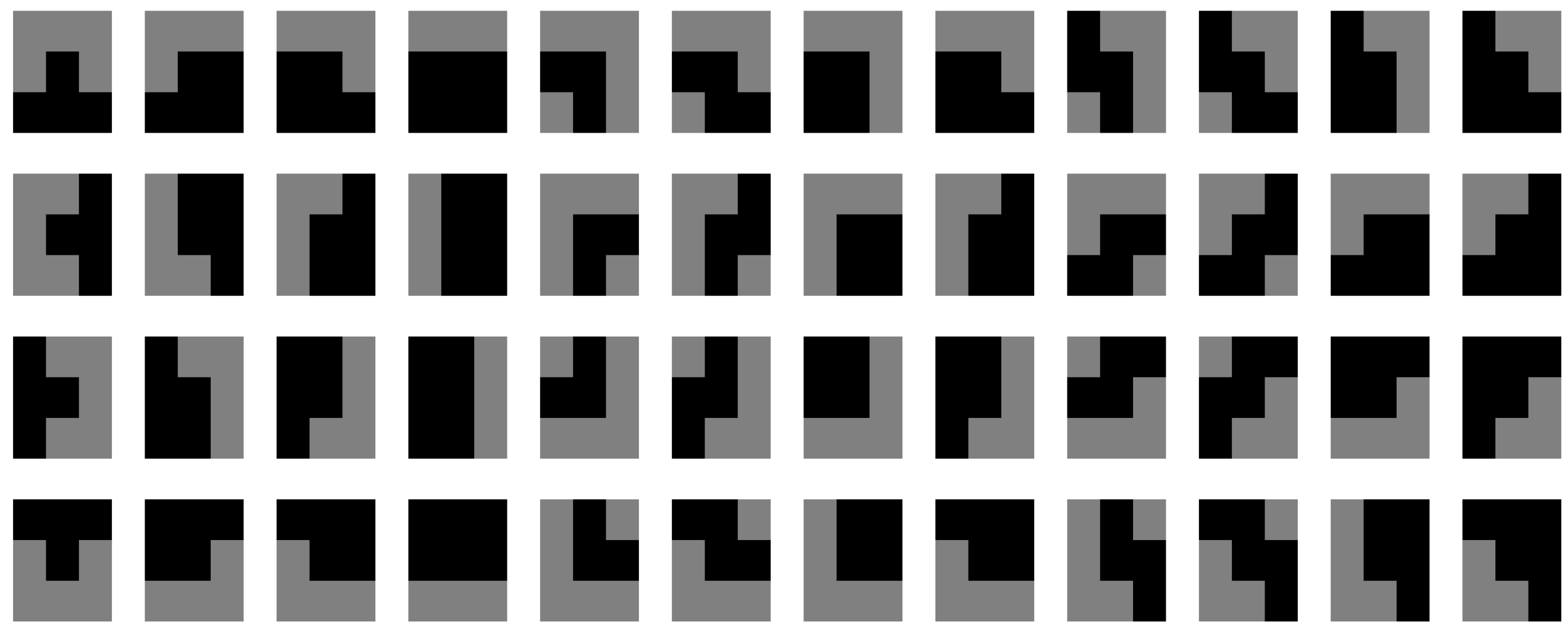
We convolve the level set function with the kernels in Equation (
1) where
denotes rotation of the matrix by a multiple
j of
radians and
,
where
. These kernals are shown in
Figure 1 We thin the segmentation of the vessels by removing the points which are centred on regions matching the above filters. That is, we set such points as background points.
We achieve this by iterating as in Equation (
2), beginning with
and cycling through
,
.
Following this, we extract the patches by cropping the image
to
pixel windows
centred on points
in the set
of points considered the foreground of the skeletonised vessel map. The patch size was selected so that bifurcations, and crossings and branches, in the vessel would fit within one patch. The patches are given by:
In the training stage, the set of patches (
) of the images in the training set are used to train the neural network to identify whether a bifurcation or crossing is contained in the image patch. In the test stage, the trained CNN classifies the patches accordingly. This step is described below.
2.3. Junction Distinction—CNN
To identify the vessel bifurcations and crossings within the patches created we train our CNN on a high-end Graphics Processor Unit (GPU). The large random access memory of the Nvidia K40c means that we were able to train on the whole dataset of patches at once. The Nvidia K40c contains 2880 CUDA cores and comes with the Nvidia CUDA Deep Neural Network library (cuDNN) for GPU learning. The deep learning package Keras [
21] was used alongside the Theano machine learning back end to implement the network. After training, the feed forward process of the CNN can classify the patches produced from a single image in under a second.
We used the Res18 network architecture [
17] as deep levels of convolution were required to distinguish the vessel junction type in our small patches. The residual layers incorporate activation, batch normalisation, convolutional, dense and maxpooling layers. We also use
regularisation to improve weight training. There were approximately 100,000 patches for training and 30,000 for testing in the junction distinction problem. The classes were weighted as a ratio of junction to background due to the fact that bifurcations and crossings in the training and testing patches were sparse at a ratio of 1:39. The network was optomised using Adam stochastic optimisation for backpropegation [
22]. The network was trained to classify the patches to give a binary classification of either vessel junction or background. Gaussian initialisation was used within the network to reduce initial training time. The loss function used for the optimisation was the widely used categorical cross-entropy function. Training was undertaken until reduction of the loss plateaued to obtain optimal results. These results can be seen in
Figure 2.
2.4. Locate the Centres
Following the neural network classification, which tell us if a bifurcation or crossing is contained within a patch, we aim to find the locations of the points.
We achieve this by forming the cumulative sum image shown in Equation (
3) and taking the local maxima
as points of interest. We then aim to determine whether points are at crossings or bifurcations.
2.5. Junction Classification
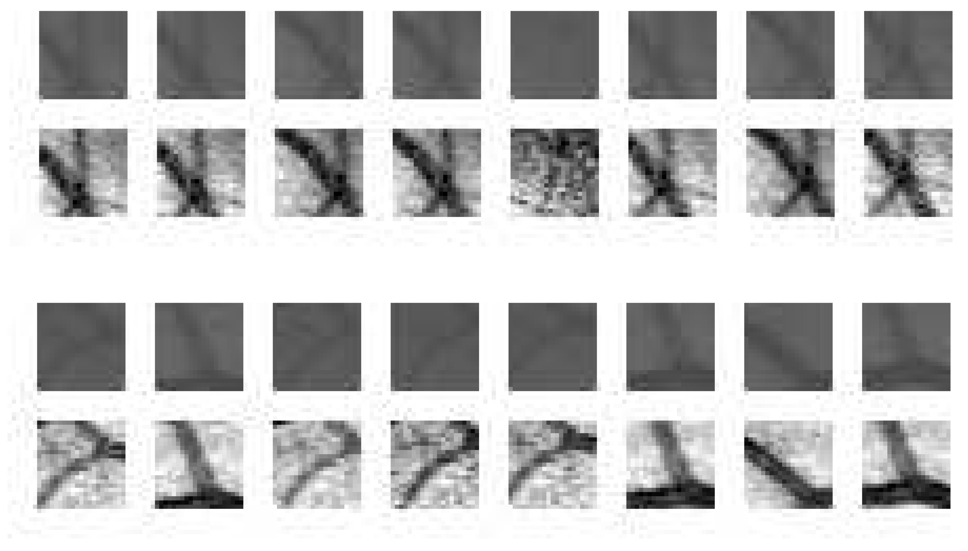
We extract the patches
and use these to train a neural network to distinguish between crossings and bifurcations as shown in
Figure 3. The second neural network was trained with the Res18 architecture, like the first. Using a relatively small training set of patches, as from our images the majority of patches did not contain bifurcations and crossings, we trained our network in similar fashion to that used in the previous step. Weighted classes were introduced again to cater for the imbalance, in that images from the bifurcation class were substantially more prominent than that of the cross class.
Depending on the patch method there were around 800–2500 patches containing a junction that was used for training which can be seen in
Figure 4. In all methods there were approximately twice as many junction patches containing bifurcation vessels compared to patches containing vessels crossing. Training was performed until a plateau in the reduction of the loss function was reached indicating no further improvement.
3. Results
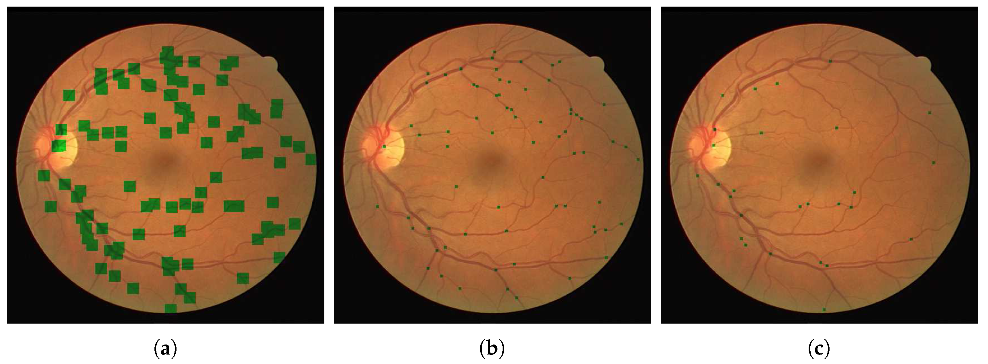
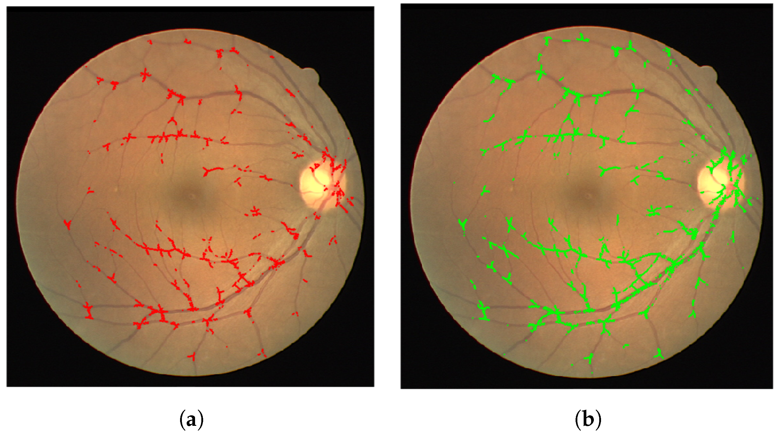
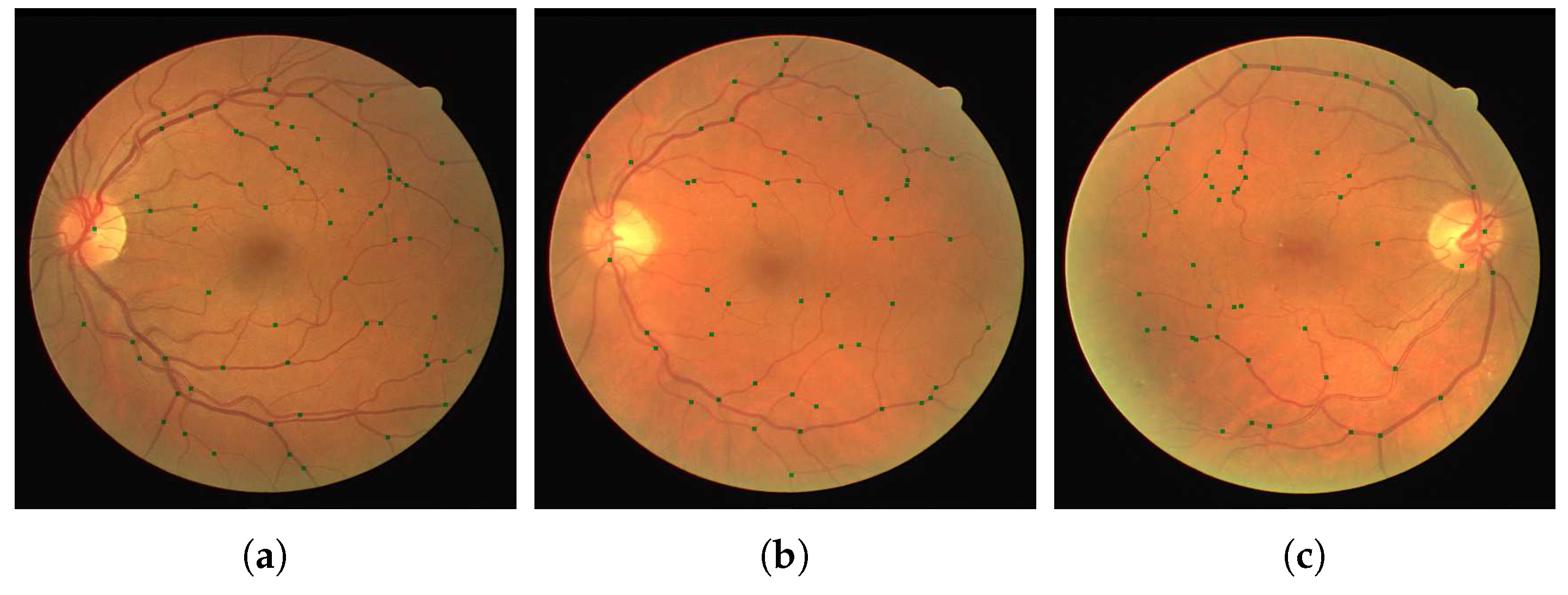
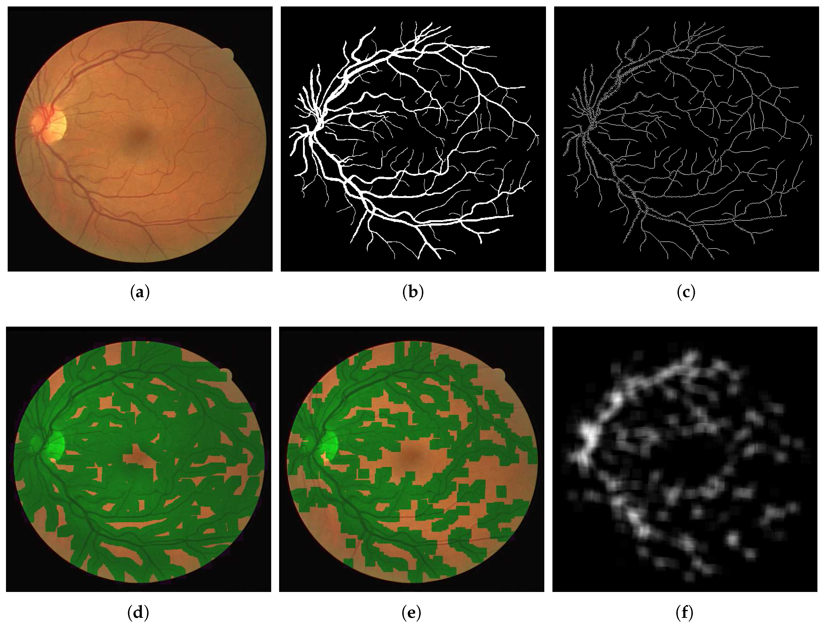
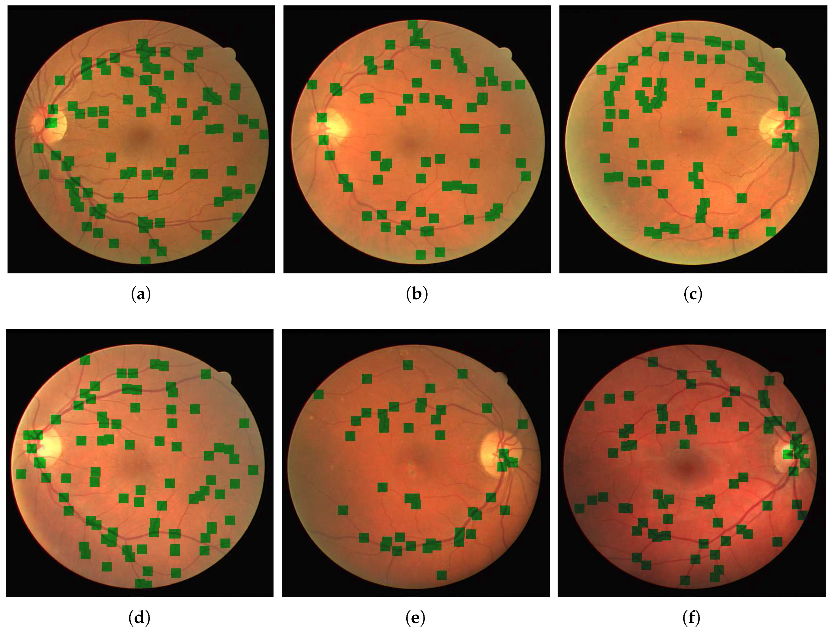
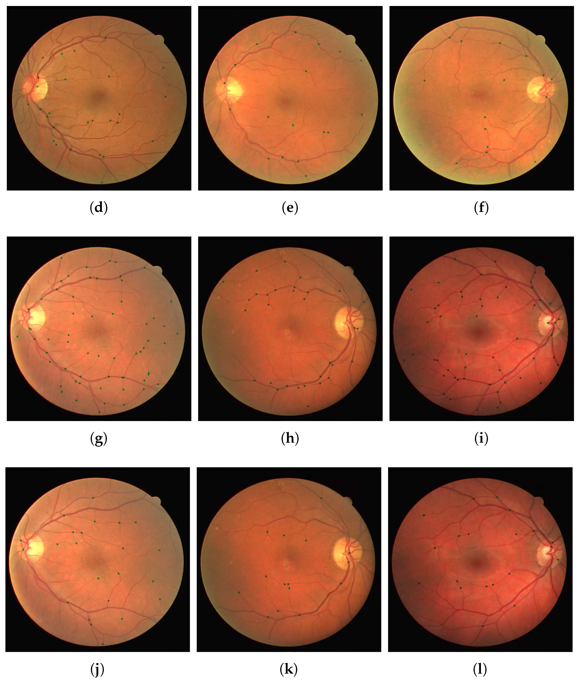
We present our results on a patch by patch basis as well as in the fundus image form with vessel bifurcations and splittings labeled. The patch detection and classification information is then used to in a probability map type reconstruction of the fundus image to produce the final appropriate vessel bifurcations and splittings, as demonstrated in
Figure 5 and
Figure 6. Here we present both the patch accuracy results and the final classified and vessel type distinguished images. We measure sensitivity, specificity and accuracy of the final image-based result as follows. Since the region of a junction is not restricted to a single point, we allow a region
of 10 pixels either side of an annotated point at
to be considered the correct region. That is, we split each image domain
into two sets
where
j denotes a junction point location.
is considered the true (junction) set and
is considered the background set. We then calculate error measures based on this and report the mean measures.
For validation we used the test images from the DRIVE dataset. Furthermore, we used the separate IOSTAR dataset, and another expert grader (G3), for testing and comparison of the patch detection and classification method. We show in
Table 1 and
Table 2 the results of training our neural networks on the data provided by graders 1, 2 and 3. In each case, we use patches extracted from 30 images from the DRIVE dataset to train our network.This relates to 101,416 patches of vessel junctions and 216,756 other patches. From the 101,416 patches there are 67,650 patches of vessel crossings and 33,766 patches of vessel bifurcations. This network is then tested by using our network to classify patches from the remaining ten images of the DRIVE dataset. This relates to 72,980 non-vessel patches and 31,026 vessel patches of which 9176 are vessel crossings and 21,850 are vessel bifurcations. We compare the results with the annotations provided by the grader in question, achieving high accuracies of 0.76, 0.76 and 0.77 for graders 1, 2 and 3 respectively. Furthermore, we use the trained network to classify images from the IOSTAR dataset, comparing with the annotations provided. With each trained network, the accuracy is lower for this unseen dataset, but the sensitivity is retained. The IOSTAR dataset gave us 132,064 non-vessel junction patches and 52,878 vessel junction patches with 14,228 vessel crossings and 38,650 vessel bifurcations. Following the detection, we resolve the patch-based results into the original images in order to identify individual junctions and to measure the detection performance for each image.
Table 3 and
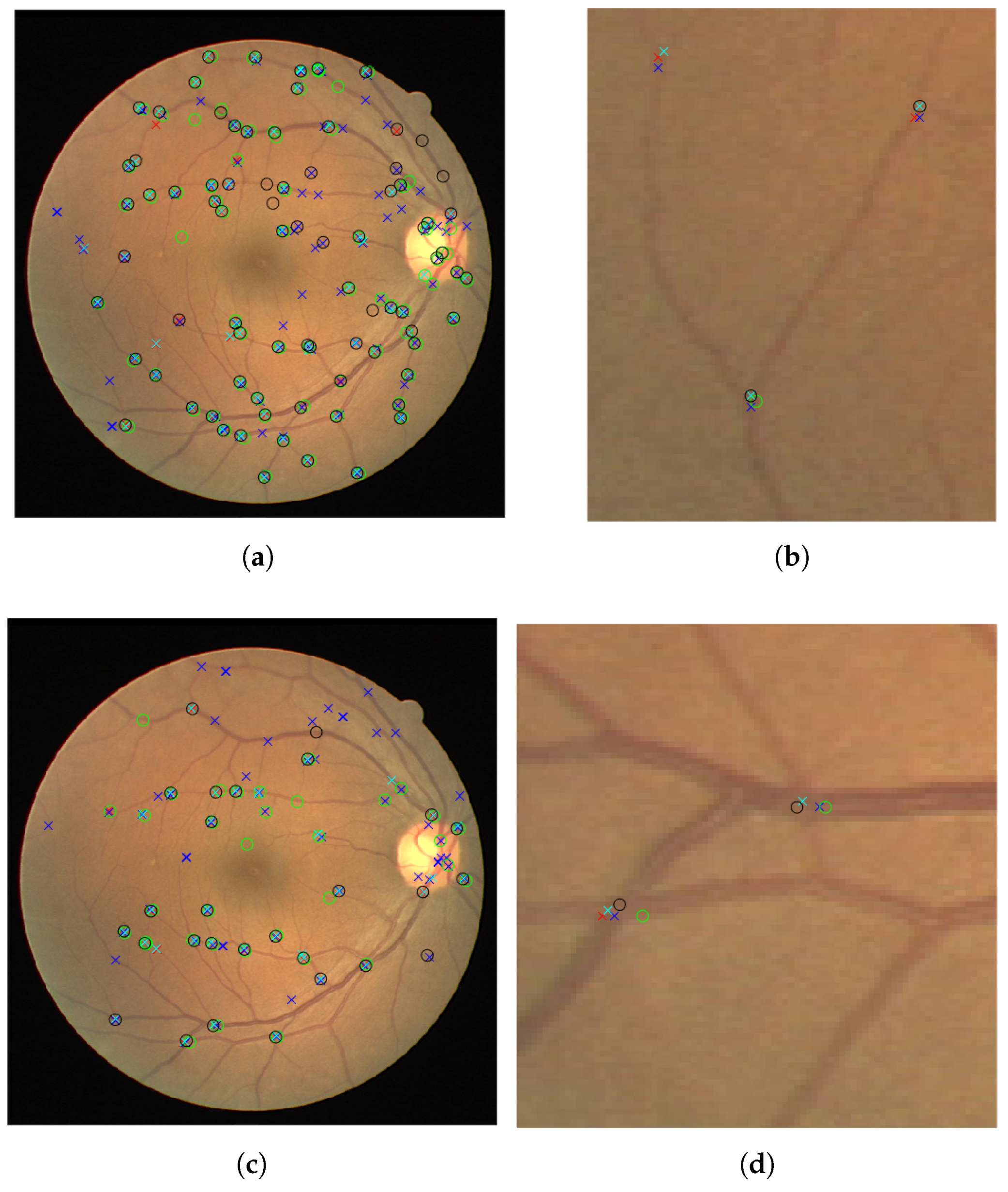
Table 4 shows the results obtained from the networks trained by the first annotations of grader 2 and grader 3 and tested on the 10 remaining test images of the DRIVE dataset. The results were compared with the annotations of grader 1 (G1A1), the first and second annotations of grader 2 (G2A1 and G2A2) as well as the first and second annotations of grader 3 (G3A1 and G3A2). Excellent performance of 81% is achieved for the network trained and tested on grader 2’s first annotation. The result is similar when comparing to the other graders. Good performance of 74% is also achieved for the network trained and tested on grader 3’s first annotation with similar, and even improved, results when comparing to other annotations. We retain good accuracy for the classification task, as shown in
Table 5 and
Figure 7 and
Figure 8, achieving accuracies of ≥0.70 for distinguishing between detected vessel crossings and bifurcations. The results were a little lower for the IOSTAR dataset but this, and the detection results, may be improved by including some of this data in the training of the networks.

 ,
, 


