


Analyzing Experimental Design and Input Data Variation of a Vanadium Redox Flow Battery Model


Abstract
:1. Introduction
2. Materials and Methods
2.1. Grey Box VRFB Model
2.2. Comparison of the Experimental Design
2.3. Comparison of Input Data Setup
- (1)
- As a basic parameter, the specification of time at measurement represents a fundamental part of the simulation model and the data set of Battery 1. Second values are needed for the simulation, therefore the data sets with specified timestamps must be converted accordingly.
- (2)
- The simulation model expects the measured AC power at the grid connection point. These data are required for the subsequent efficiency analysis and is only recorded for the measurement series with 15 A charge and discharge current. A defect at the converter makes further recordings impossible. The measured values recorded up to that point are not plausible. Due to the current data situation, which cannot be extended, there is no efficiency analysis and this part of the model is not used within this study.
- (3)
- To determine the optimization parameters, a modified formula from Nernst equation is applied, which describes the battery model as one of the three main equations. Battery 2 provides a calculated SOC through its integrated BMS, which can be passed to the simulation model. Battery 1, on the other hand, does not have this function and data, which is why several options for modifying the input data and determining the SOC were explained in the next chapter.
- (4)
- Differences are found in the data sets for the voltages and currents at the stacks. The model calculates with the total voltage, which represents the average voltage of both stacks. The data sets of Battery 1 only provide the individual stack voltages which would allow a simulation, but only with the voltage of one stack. Since the stacks are usually electrically connected in parallel, the voltage values differ only slightly. Thus, a mathematical adjustment of both stack voltages of Battery 1 takes place by forming the average value from both stacks.
- (5)
- If the total capacity of the battery is to be determined, the total current must be entered into the simulation. The data set of Battery 1 provides the current per stack, which is why a conversion is made to obtain the total current. As another part of the simulation model, a smoothing of certain raw data takes place. Unlike the raw Battery 2 data used in development, Battery 1 is current driven. The scatter of the current values of Battery 2 is therefore much smaller. However, no changes are made in this respect, since the functionality is also maintained with the raw data of Battery 1.
- (6)
- The simulation model offers the possibility to perform the calculations depending on the temperature value of the electrolyte. For this purpose, this value is read in via the last column of the input data set. However, since the battery system of Battery 1 does not record a temperature value, this is left out for later consideration. A constant value of 295.15 K (23 °C) is assumed for the temperature.
2.4. Methods for Obtaining the SOC
2.4.1. Discharge Test
2.4.2. Ampere Counting
2.4.3. SOC–OCV Relation
3. Results and Discussion
3.1. OCV–SOC Conversion Results
3.2. Parametrization and Optimization of the Redox Flow Model
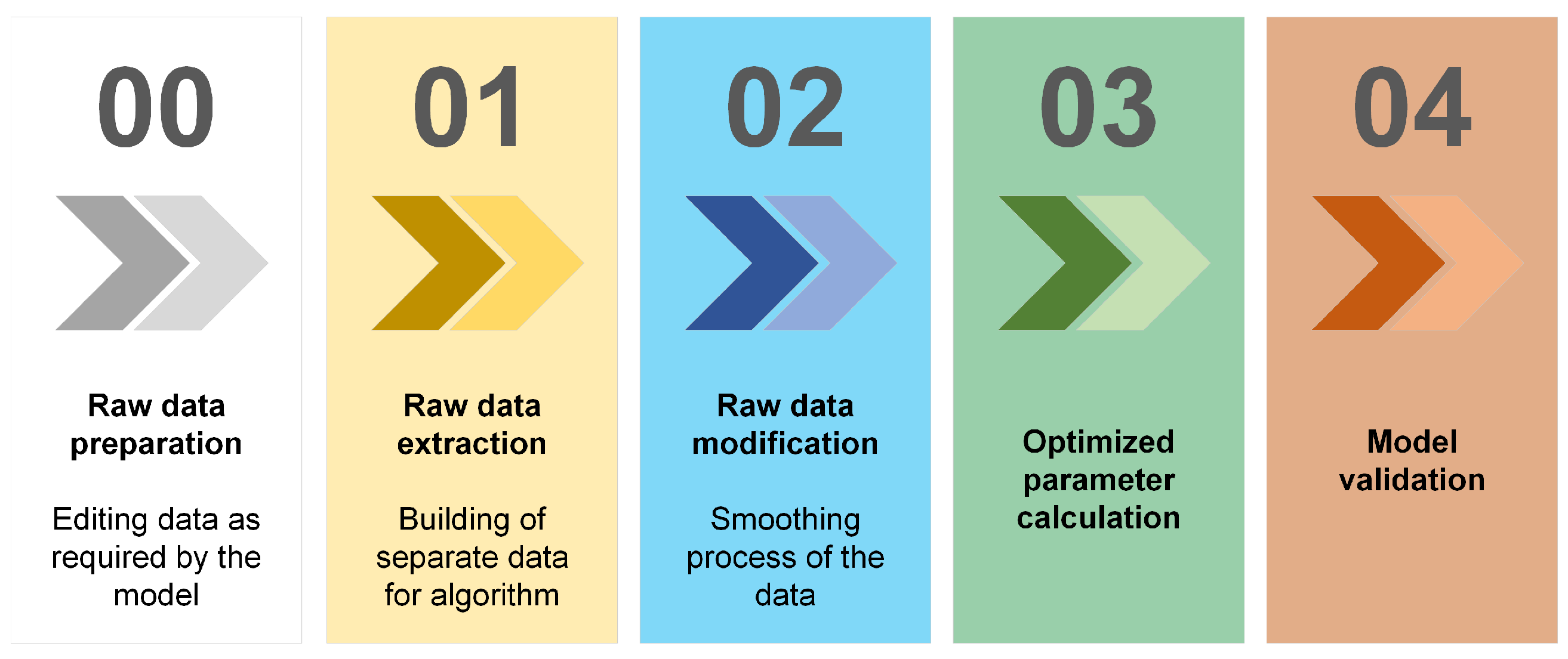
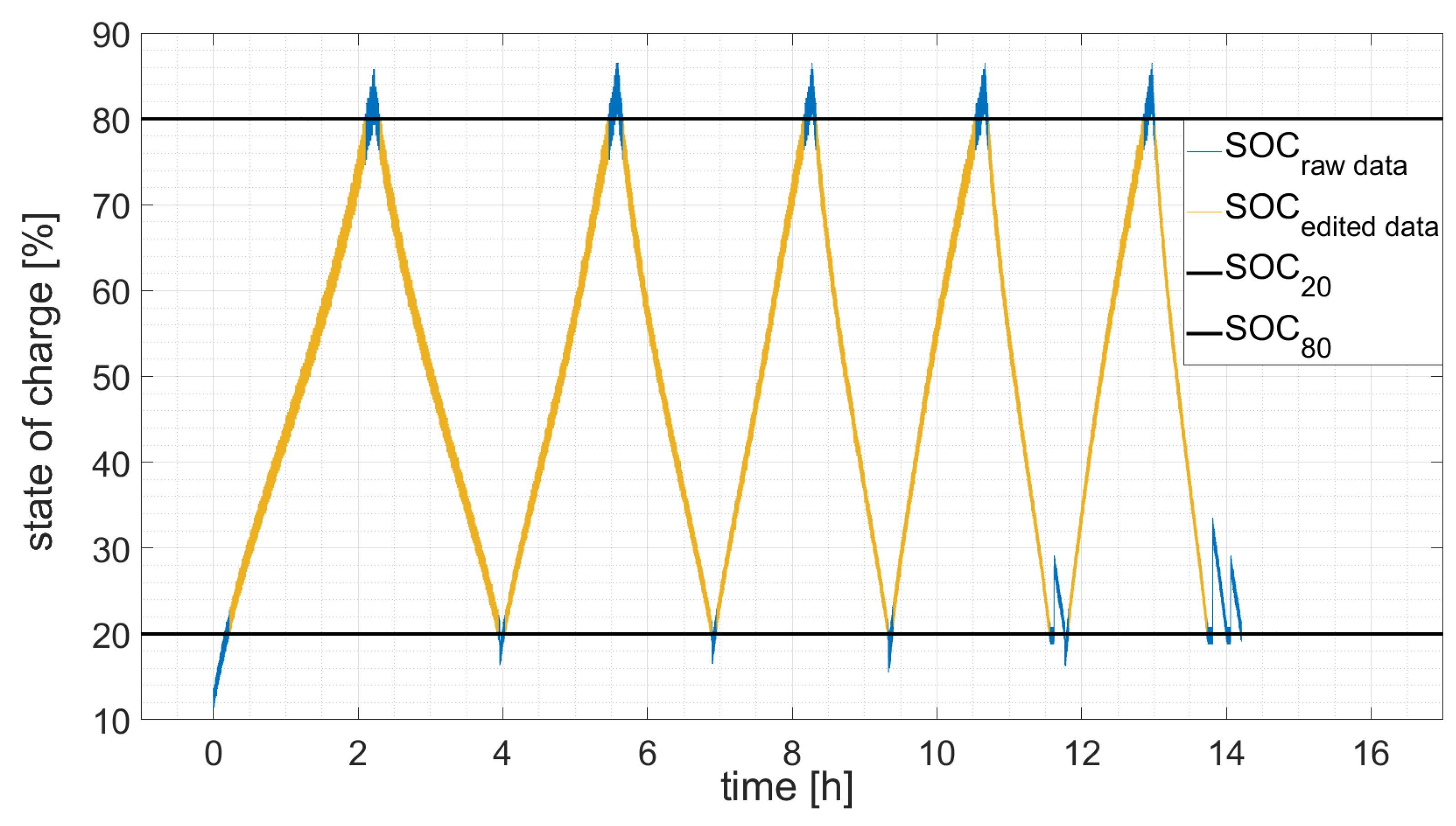
3.2.1. Raw Data Extaction
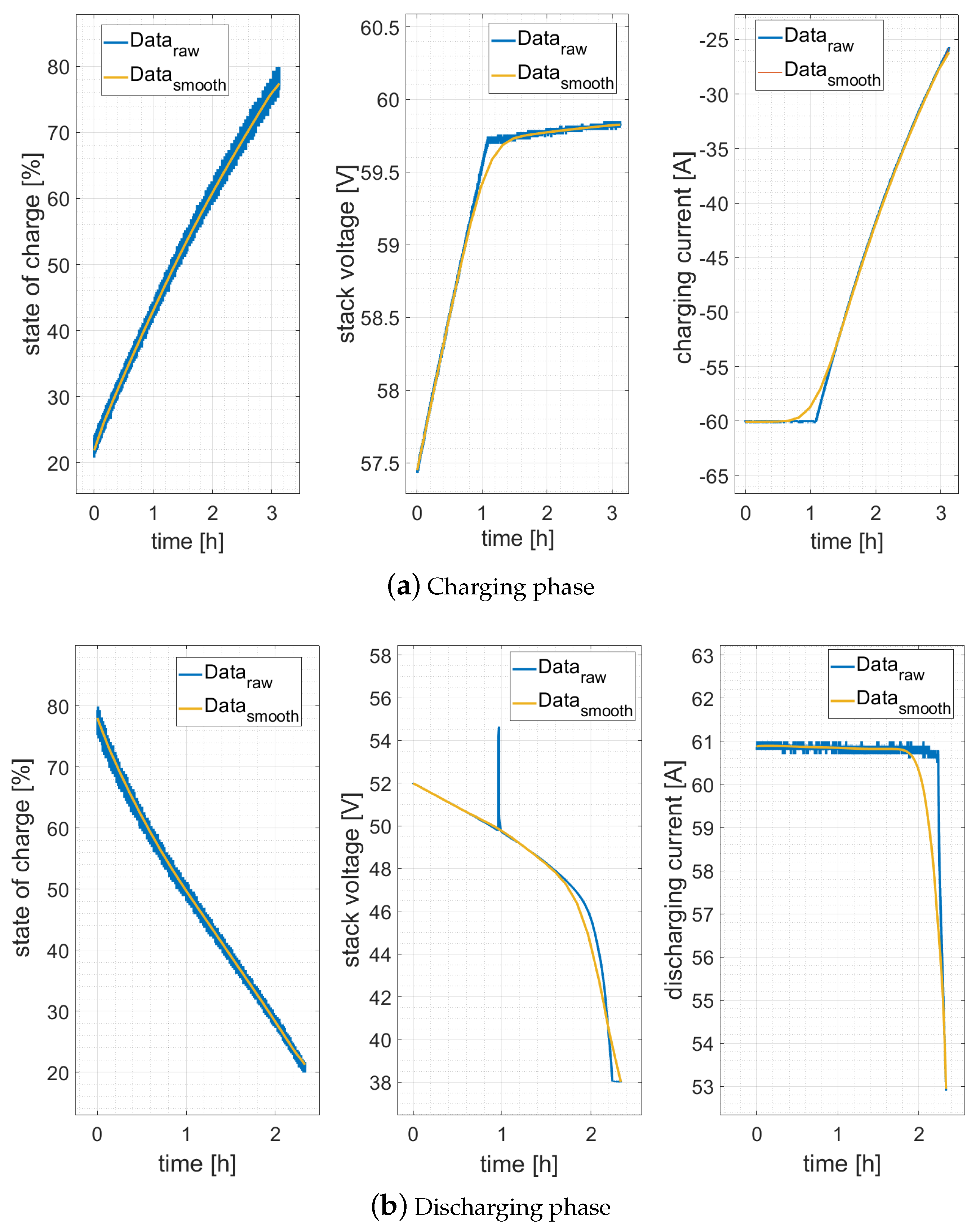
3.2.2. Raw Data Modification
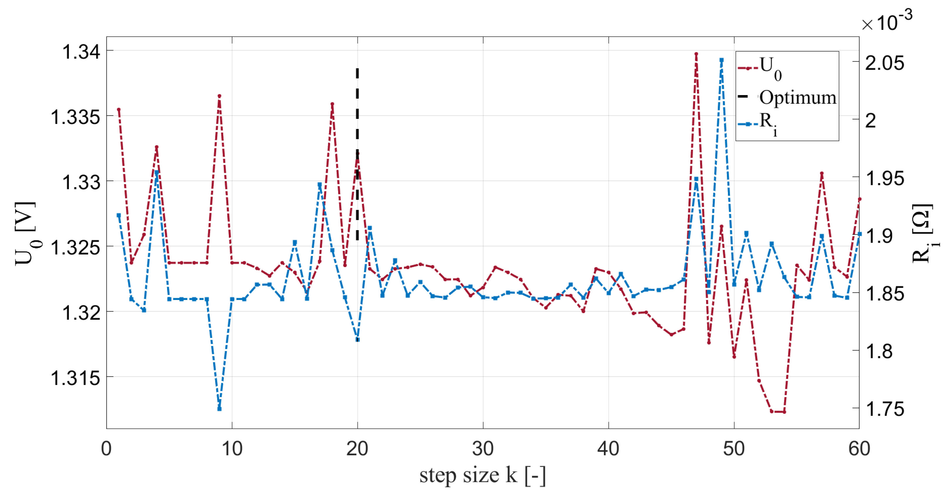
3.2.3. Calculating the Optimization Parameters
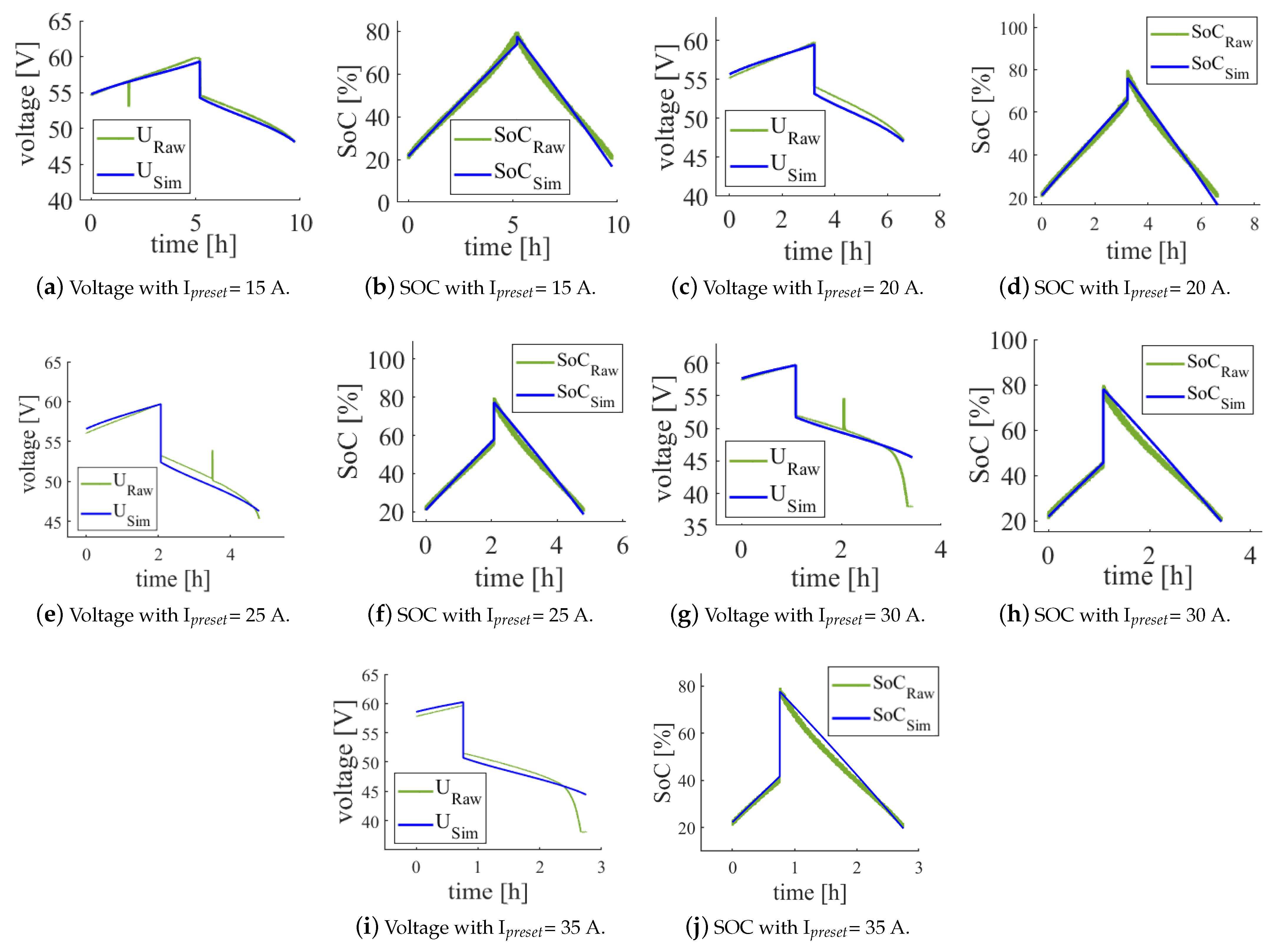
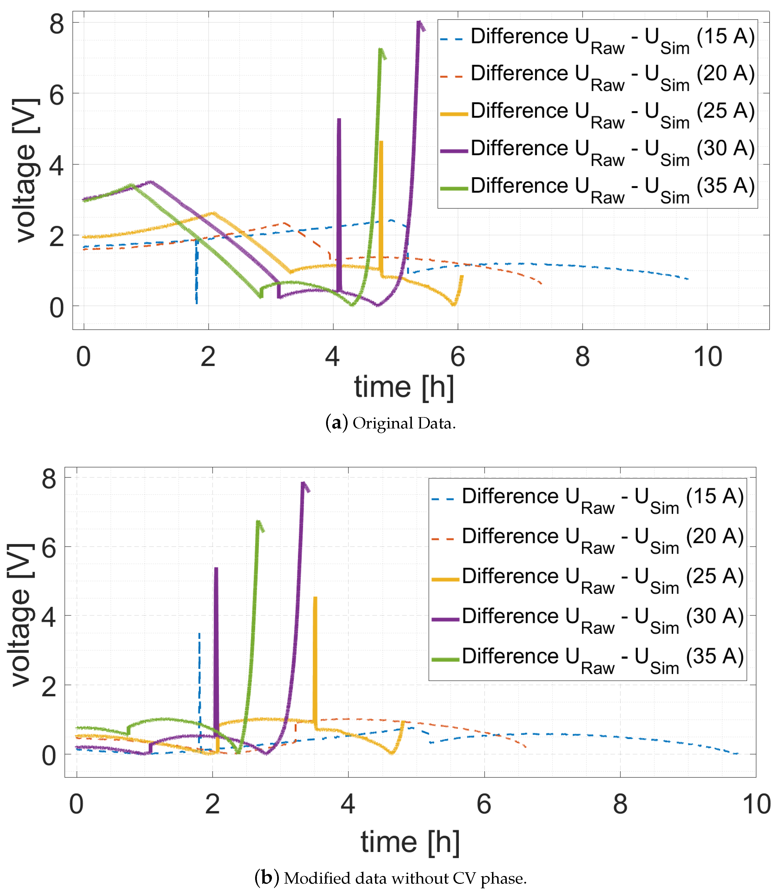
3.3. Validation of the Simulation with Real Measurement
4. Conclusions
Author Contributions
Funding
Data Availability Statement
Conflicts of Interest
Abbreviations
| CC | Constant Current |
| CV | Constant Voltage |
| BMS | Battery Management System |
| OCV | Open Circuit Voltage |
| RE | Renewable Energy |
| RFB | Redox Flow Battery |
| SOC | State of Charge |
| VRFB | Vanadium Redox Flow Battery |
References
- Zugschwert, C.; Dundálek, J.; Leyer, S.; Hadji-Minaglou, J.R.; Kosek, J.; Pettinger, K.H. The Effect of Input Parameter Variation on the Accuracy of a Vanadium Redox Flow Battery Simulation Model. Batteries 2021, 7, 7. [Google Scholar] [CrossRef]
- Elavarasan, R.M.; Shafiullah, G.M.; Padmanaban, S.; Kumar, N.M.; Annam, A.; Vetrichelvan, A.M.; Mihet-Popa, L.; Holm-Nielsen, J.B. A Comprehensive Review on Renewable Energy Development, Challenges, and Policies of Leading Indian States with an International Perspective. IEEE Access 2020, 8, 74432–74457. [Google Scholar] [CrossRef]
- Flannery, T.; Hughes, L.; Steffen, W.; Morgan, W.; Dean, A.; Smith, R.; Baxter, T. From Paris to Glasgow: A World on the Move; Climate Council: Sidney, Australia, 2021; ISBN 978-1-922404-37-4. [Google Scholar]
- Aneke, M.; Wang, M. Energy storage technologies and real life applications—A state of the art review. Appl. Energy 2016, 179, 350–377. [Google Scholar] [CrossRef]
- Maria, S.K.; Miron, R.; Robert, R. All-Vanadium Redox. Battery. Patent number US4786567A, 11 February 1986. [Google Scholar]
- Lucas, A.; Chondrogiannis, S. Smart grid energy storage controller for frequency regulation and peak shaving, using a vanadium redox flow battery. Int. J. Electr. Power Energy Syst. 2016, 80, 26–36. [Google Scholar] [CrossRef]
- Viswanathan, V.; Crawford, A.; Stephenson, D.; Kim, S.; Wang, W.; Li, B.; Coffey, G.; Thomsen, E.; Graff, G.; Balducci, P.; et al. Cost and performance model for redox flow batteries. J. Power Sources 2014, 247, 1040–1051. [Google Scholar] [CrossRef]
- Parasuraman, A.; Lim, T.M.; Menictas, C.; Skyllas-Kazacos, M. Review of material research and development for vanadium redox flow battery applications. Electrochim. Acta 2013, 101, 27–40. [Google Scholar] [CrossRef]
- Christina Zugschwert. Evaluation von Synergieeffekten Zentraler Speichersysteme in Niederspannungsnetzen Durch Integrative Modellbildung. Ph.D. Thesis, Université du Luxembourg, Luxembourg, 2022.
- Robert Labus. Teststandsoptimierung für eine Vanadium-Redox-Flow-Batterie unter Einbezug der Erfassung thermischer und Elektrischer Systemparameter. Master’s Thesis, Hochschule für angewandte Wissenschaften Landshut, Landshut, Germany, 2020.
- Volterion GmbH. Datenblatt—Vanadium Redox Flow Battery VRFB 11/12; Volterion GmbH: Dortmund, Germany, 2018. [Google Scholar]
- Gildemeister Energy Solutions. Datenblatt—Vanadium Redox Flow Battery FB10-100; Gildemeister Energy Solutions: Wiener Neudorf, Austria, 2012. [Google Scholar]
- Wei, L.; Zhao, T.S.; Xu, Q.; Zhou, X.L.; Zhang, Z.H. In-situ investigation of hydrogen evolution behavior in vanadium redox flow batteries. Appl. Energy 2017, 190, 1112–1118. [Google Scholar] [CrossRef]
- Piller, S.; Perrin, M.; Jossen, A. Methods for state-of-charge determination and their applications. J. Power Sources 2001, 96, 113–120. [Google Scholar] [CrossRef]
- Skyllas-Kazacos, M.; Kazacos, M. State of charge monitoring methods for vanadium redox flow battery control. J. Power Sources 2011, 196, 8822–8827. [Google Scholar] [CrossRef]
- Knehr, K.W.; Kumbur, E.C. Open circuit voltage of vanadium redox flow batteries: Discrepancy between models and experiments. Electrochem. Commun. 2011, 13, 342–345. [Google Scholar] [CrossRef]
- Corcuera, S.; Skyllas-Kazacos, M. State-of-Charge Monitoring and Electrolyte Rebalancing Methods for the Vanadium Redox Flow Battery. Eur. Chem. Bull. 2012, 1, 511–519. [Google Scholar] [CrossRef]
- König, S. Model-Based Design and Optimization of Vanadium Redox Flow Batteries. Ph.D. Thesis, Karlsruher Institut für Technologie, Karlsruhe, Germany, 2017. [Google Scholar] [CrossRef]
- Fathima, A.H.; Palanismay, K. Modeling and Operation of a Vanadium Redox Flow Battery for PV Applications. Energy Procedia 2017, 117, 607–614. [Google Scholar] [CrossRef]
- Shin, K.H.; Jin, C.S.; So, J.Y.; Park, S.K.; Kim, D.H.; Yeon, S.H. Real-time monitoring of the state of charge (SOC) in vanadium redox-flow batteries using UV–Vis spectroscopy in operando mode. J. Energy Storage 2020, 27, 101066. [Google Scholar] [CrossRef]
- Hudak, N.S. Practical thermodynamic quantities for aqueous vanadium- and iron-based flow batteries. J. Power Sources 2014, 269, 962–974. [Google Scholar] [CrossRef]
- Bard, A.J.; Faulkner, L.R. Electrochemical Methods: Fundamentals and Applications, 2nd ed.; Wiley: New York, NY, USA; Weinheim, Germany, 2001. [Google Scholar]
- Guidelli, R.; Piccardi, G.; Moncelli, M.R. Mechanism of electrohydrodimerization of diactivated olefins in aqueous media. J. Electroanal. Chem. Interfacial Electrochem. 1981, 129, 373–378. [Google Scholar] [CrossRef]
- Wei, Z.; Lim, T.M.; Skyllas-Kazacos, M.; Wai, N.; Tseng, K.J. Online state of charge and model parameter co-estimation based on a novel multi-timescale estimator for vanadium redox flow battery. Appl. Energy 2016, 172, 169–179. [Google Scholar] [CrossRef]
- Mohamed, M.R.; Leung, P.K.; Sulaiman, M.H. Performance characterization of a vanadium redox flow battery at different operating parameters under a standardized test-bed system. Appl. Energy 2015, 137, 402–412. [Google Scholar] [CrossRef]
- Noack, J.; Wietschel, L.; Roznyatovskaya, N.; Pinkwart, K.; Tübke, J. Techno-Economic Modeling and Analysis of Redox Flow Battery Systems. Energies 2016, 9, 627. [Google Scholar] [CrossRef]
- Huang, Z.; Mu, A. Research and analysis of performance improvement of vanadium redox flow battery in microgrid: A technology review. Int. J. Energy Res. 2021, 45, 14170–14193. [Google Scholar] [CrossRef]
- Zhang, Y.; Zhao, J.; Wang, P.; Skyllas-Kazacos, M.; Xiong, B.; Badrinarayanan, R. A comprehensive equivalent circuit model of all-vanadium redox flow battery for power system analysis. J. Power Sources 2015, 290, 14–24. [Google Scholar] [CrossRef]
- Kim, S.; Thomsen, E.; Xia, G.; Nie, Z.; Bao, J.; Recknagle, K.; Wang, W.; Viswanathan, V.; Luo, Q.; Wei, X.; et al. 1 kW/1 kWh advanced vanadium redox flow battery utilizing mixed acid electrolytes. J. Power Sources 2013, 237, 300–309. [Google Scholar] [CrossRef]
- Bard, A.J.; Faulkner, L.R.; White, H.S. Electrochemical Methods: Fundamentals and Applications, 3rd ed.; Wiley: Hoboken, NJ, USA, 2022. [Google Scholar]


| Battery 1 | Battery 2 | |
|---|---|---|
| Model name | Volterion VRFB 11 | CellCube FB 10–100 |
| Stack configuration | 2 stacks | 10 stacks |
| Nominal power | 5 kW | 10 kW |
| Overall capacity | 10 kWh | 100 kWh |
| Nominal voltage | 48 V | 48 V |
| Considered SOC boundaries | 20–80% | 20–80% |
| Temperature range | 0–40 °C | 20–30 °C |
| Number | VRFB Simulation Model | Battery 1 Data Set |
|---|---|---|
| 1 | Absolute time [s] | Time stamp [hh:mm:ss] |
| 2 | Grid side power AC [W] | - |
| 3 | SOC [%] | - |
| 4 | Total stack voltage [V] | Voltage per stack [V] |
| 5 | Total stack current [A] | Current per stack [A] |
| 6 | Temperature [°C] | - |
| Preset Charge and Discharge Current | Linear Equation | OCV at 20% SOC | OCV at 80% SOC |
|---|---|---|---|
| 15 A | OCV = 0.253x + 1.245 | 1.296 V | 1.448 V |
| 20 A | OCV = 0.260x + 1.243 | 1.295 V | 1.451 V |
| 25 A | OCV = 0.260x + 1.243 | 1.296 V | 1.456 V |
| 30 A | OCV = 0.258x + 1.253 | 1.395 V | 1.459 V |
| 35 A | OCV = 0.256x + 1.247 | 1.307 V | 1.460 V |
| Current Values [1] | New Values | |
|---|---|---|
| Total capacity C [As] | 8,700,000 (2416.67 Ah) | 1,000,000 (277.78 Ah) |
| Current loss I [A] | 10.0 | 2.0 |
| Cell voltage U [V] | 1.375 | 1.2 |
| Cell resistance R [] | 0.00075 | 0.0010 |
| Loop index [%] | 5 | 50 |
| Step size k [-] | 30 | 30 |
| With CV Phase | Without CV Phase | |
|---|---|---|
| Total capacity C [Ah] | 255.66 | 255.01 |
| Current loss I [A] | 4.24 | 3.83 |
| Cell voltage U [V] | 1.33 | 1.36 |
| Cell resistance R [] | 0.0018 | 0.0024 |
Disclaimer/Publisher’s Note: The statements, opinions and data contained in all publications are solely those of the individual author(s) and contributor(s) and not of MDPI and/or the editor(s). MDPI and/or the editor(s) disclaim responsibility for any injury to people or property resulting from any ideas, methods, instructions or products referred to in the content. |
© 2023 by the authors. Licensee MDPI, Basel, Switzerland. This article is an open access article distributed under the terms and conditions of the Creative Commons Attribution (CC BY) license (https://creativecommons.org/licenses/by/4.0/).
Share and Cite
Weber, R.; Schubert, C.; Poisl, B.; Pettinger, K.-H. Analyzing Experimental Design and Input Data Variation of a Vanadium Redox Flow Battery Model. Batteries 2023, 9, 122. https://doi.org/10.3390/batteries9020122
Weber R, Schubert C, Poisl B, Pettinger K-H. Analyzing Experimental Design and Input Data Variation of a Vanadium Redox Flow Battery Model. Batteries. 2023; 9(2):122. https://doi.org/10.3390/batteries9020122
Chicago/Turabian StyleWeber, Robert, Christina Schubert, Barbara Poisl, and Karl-Heinz Pettinger. 2023. "Analyzing Experimental Design and Input Data Variation of a Vanadium Redox Flow Battery Model" Batteries 9, no. 2: 122. https://doi.org/10.3390/batteries9020122
APA StyleWeber, R., Schubert, C., Poisl, B., & Pettinger, K.-H. (2023). Analyzing Experimental Design and Input Data Variation of a Vanadium Redox Flow Battery Model. Batteries, 9(2), 122. https://doi.org/10.3390/batteries9020122