
Calculation of Constant Power Lithium Battery Discharge Curves


Abstract
:1. Introduction
2. Theoretical Development
- (1)
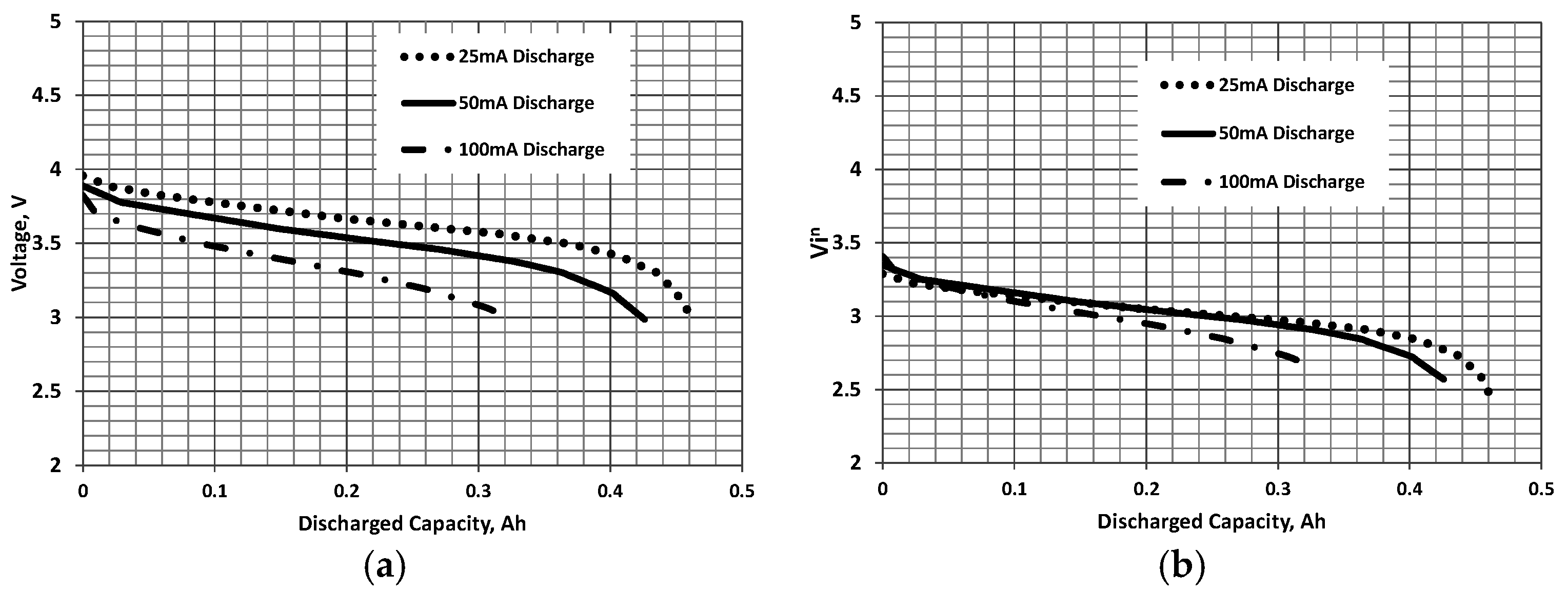
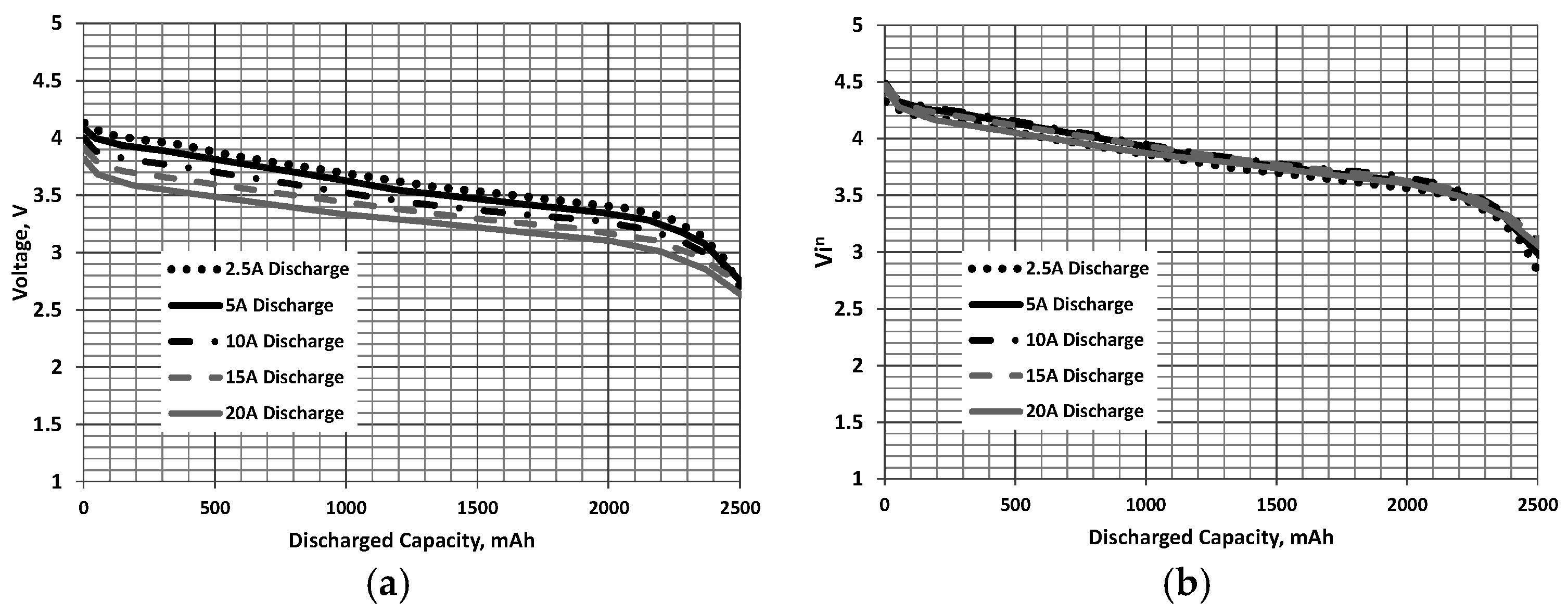
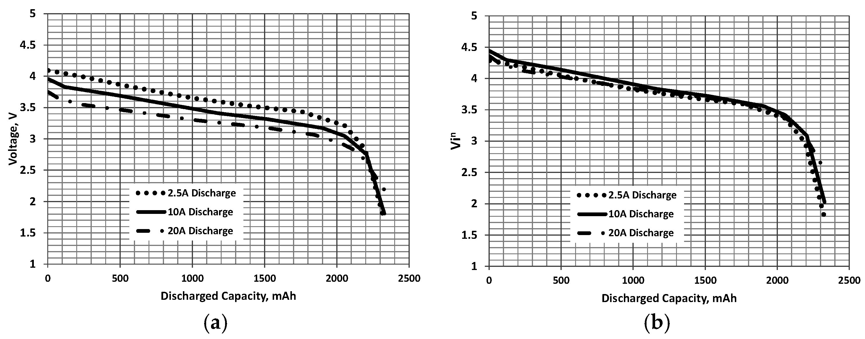
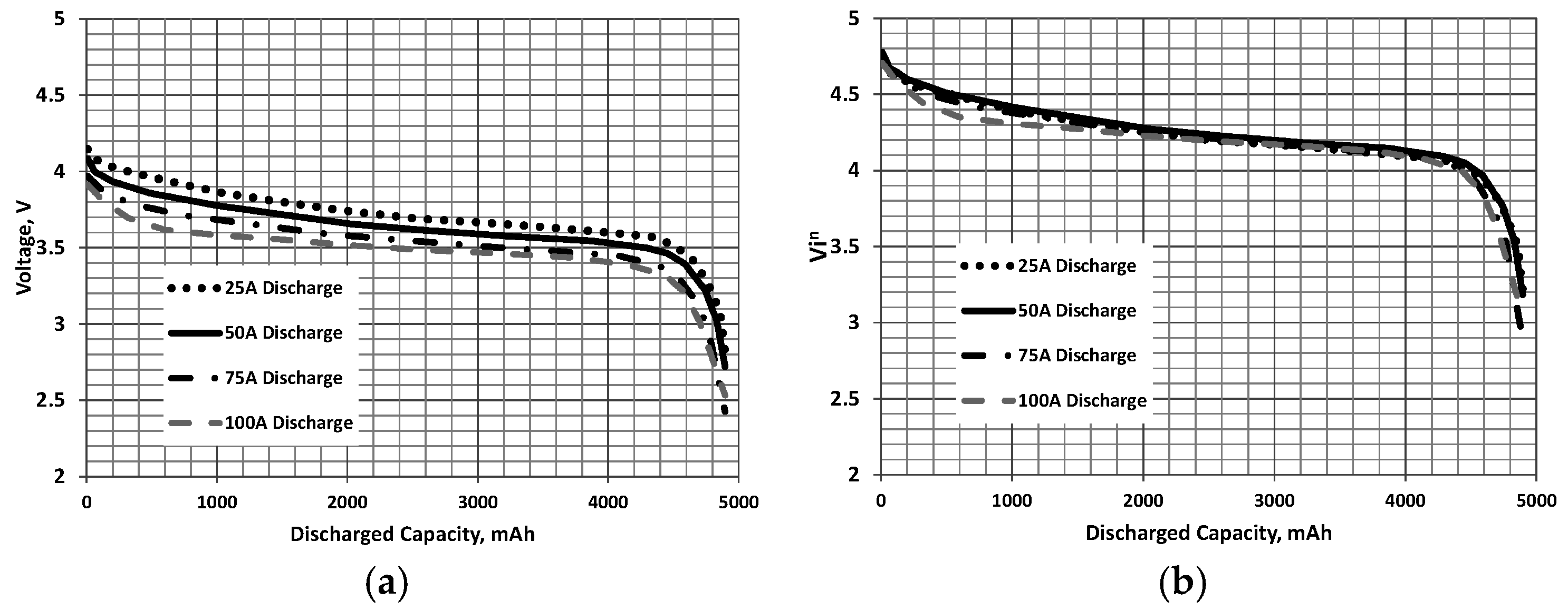
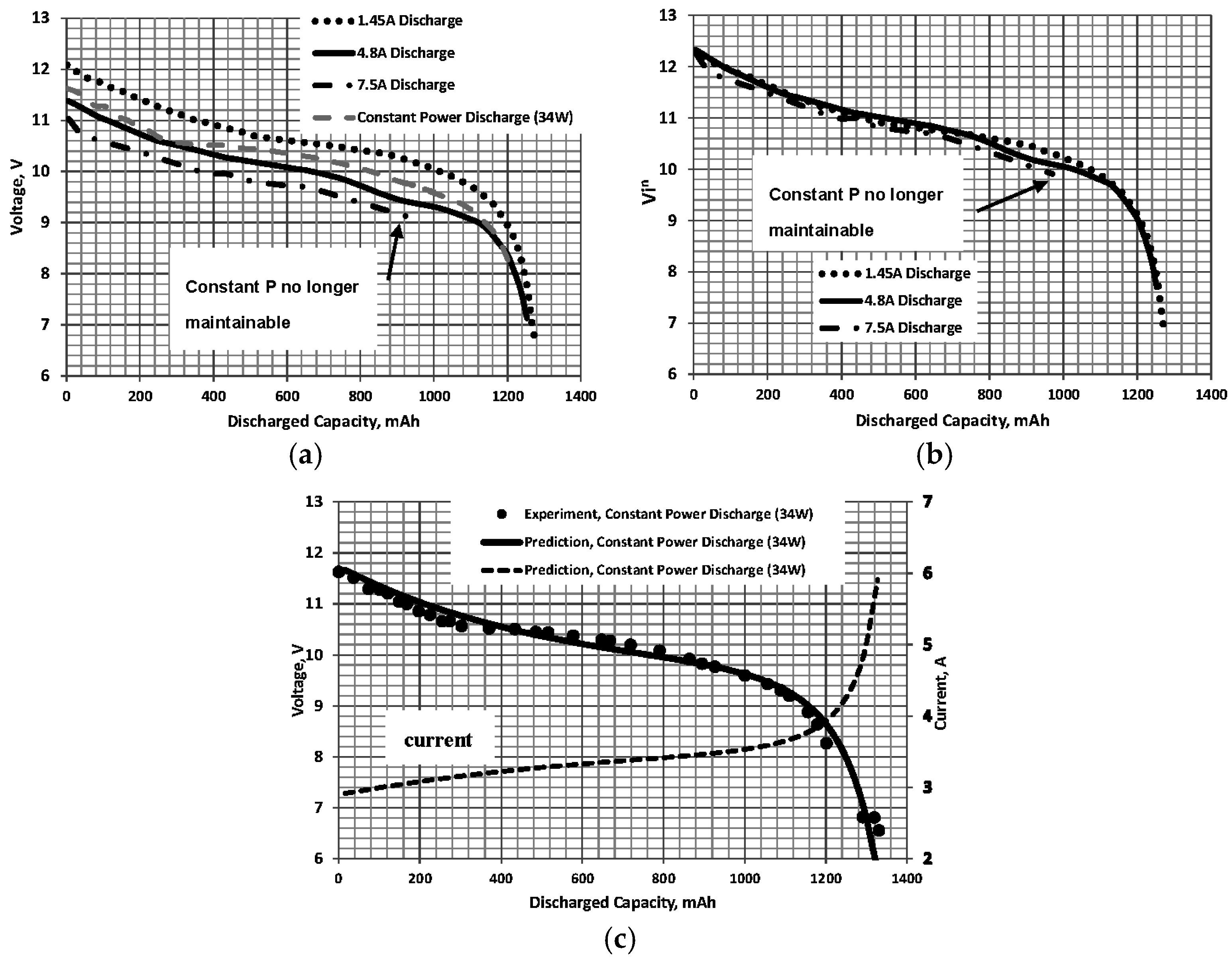
- Using the available constant current discharge curves for the battery of interest, plot inV as a function of the discharged capacity, D, see Figure 1b, Figure 2b and Figure 3b for examples. Adjust n to afford the best collapse of the curves. Alternatively, n may be established using a non-linear least square minimization as follows. Let M = the number of test cases (discharges at different i for a given battery). The least square criterion is implemented as:where the overbar indicates an average for all j (for a discharge D). The counter j refers to the individual data sets. A non-linear least square solver (found in MS Excel, or most mathematical computational software) may be used to find the value of n that minimizes the summation.
- (2)
- Once n has been determined, the collapsed plots are curve fitted as a function of D. A function of the form:matches a battery discharge curve profile well and can be readily found using software such as TableCurve, MathCad or most statistical curve fitting packages. Naturally, other curve fit functions may also be used. Note that the non-linear least square minimization solver may be used directly to solve Equations (3) and (4) with the form of the curve fit expressed by Equation (4) prescribed. However, ill-conditioning and divergence may be an issue unless the initial estimates of the coefficients in Equation (4) are close to the optimal values.
- (3)
- The voltage during the discharge may be found using which after substitution of yields:note that for the calculations to not be circular, Vj cannot be a function of inV(D)j. It is thus assumed that inV(D)j = inV(D)j−1 for each successive step, not for successive steps. What this implies is that inV(D) does not change rapidly between each iteration. As long as the time step is small relative to the total discharge time this is a reasonable assumption. If the required Preq or mechanical power is known, then Pe = Preq/ηtot where ηtot is the efficiency of the propulsion system including the propeller, electronic speed controller and motor.
- (4)
- The corresponding current at this time step is:
- (5)
- The discharged capacity then follows as:
- (6)
- Calculate the voltage, current and discharged capacity at the next time step t (t(h) = j/N where j = 1, 2, 3, ... and N is an arbitrary constant defining the time step increment. In this article N = 180 giving time increments Δt of 20 s). The time step should be small compared to the discharge duration to ensure the validity of Equation (5).
- (7)
- Repeat Steps 3–5 until the discharged capacity Dj is approximately equal to C.
3. Materials and Methods
4. Discussion
- The time increment is given by 1/180 = 0.0056 h (20 s);
- From Equation (5) with j = 1: = 11.67 V; and
- Equation (6) gives: = 2.914 A;
- The discharged capacity follows from Equation (7) as: D1 = i1Δt + D0 = 2.914 × 103 × (0.00556) + 0 = 16.202 mAh;
- Advancing j = 2 and evaluating Equations (5)–(7) yields V2 = 11.601 V, i2 = 2.931 A and D2 = 32.498 mAh.
5. Conclusions
Conflicts of Interest
Abbreviations
| C | Capacity |
| D | Discharged capacity |
| e | Electrical |
| i | Current |
| j | Counter |
| K | Constant |
| M | Number of test cases |
| N | Time step increment |
| n | Exponent |
| P | Power |
| t | Time |
| V | Voltage |
| ηtot | Total efficiency of propulsion system |
References
- Lawrence, D.A.; Mohseni, K. Efficiency Analysis for Long-Duration Electric MAVs. In Proceedings of the Infotech@Aerospace Conferences, Arlington, VA, USA, 26–29 September 2005. [CrossRef]
- Gur, O.; Rosen, A. Optimizing electric propulsion systems for unmanned aerial vehicles. J. Aircr. 2009, 46, 1340–1353. [Google Scholar] [CrossRef]
- Ostler, J.N. Flight Testing Small Electric Powered Unmanned Aerial Vehicles. Master’s Thesis, Brigham Young University, Provo, UT, USA, April 2006. [Google Scholar]
- Retana, E.R.; Rodrigue-Cortes, H. Basic Small Fixed Wing Aircraft Sizing Optimizing Endurance. In Proceedings of the 4th International Conference on Electrical and Electronics Engineering (ICEEE), Mexico City, Mexico, 5–7 September 2007; pp. 322–325.
- Anderson, J.D. Aircraft Performance, 1st ed.; McGraw Hill: Columbus, OH, USA, 1999; pp. 293–300. [Google Scholar]
- McCormick, B.W. Aerodynamics, Aeronautics and Flight Mechanics; Wiley: New York, NY, USA, 1995; pp. 378–385. [Google Scholar]
- Hale, F. Introduction to Aircraft Performance, Selection and Design; Wiley: Hoboken, NJ, USA, 1984; pp. 123–129. [Google Scholar]
- Traub, L.W. Range and endurance estimates for battery powered aircraft. J. Aircr. 2011, 48, 703–707. [Google Scholar] [CrossRef]
- Traub, L.W. Validation of endurance estimates for battery powered UAVs. Aeronaut. J. 2013, 117, 1155–1166. [Google Scholar] [CrossRef]
- Peukert, W. Über die Abhängigkeit der Kapazität von der Entladestromstärke bei Bleiakkumulatoren. Elektrotech. Z. 1897, 20, 287–288. (In German) [Google Scholar]
- Su, Y.; Liahng, H.; Wu, J. Multilevel Peukert Equations Based Residual Capacity Estimation Method for Lead-Acid Batteries. In Proceedings of the 2008 IEEE International Conference on Sustainable Energy Technologies, Singapore, 24–27 November 2008; pp. 101–105.
- Andrea, D. Battery Management Systems for Large Lithium Ion Battery Packs, 1st ed.; Artech House: Norwood, MA, USA, 2010. [Google Scholar]
- Sony. Lithium Ion Rechargeable Batteries Technical Handbook. Available online: http://www.dlnmh9ip6v2uc.cloudfront.net/datasheets/Prototyping/Lithium%20Ion%20Battery%20MSDS.pdf (accessed on 15 September 2015).
- Sanyo. Lithium Ion Handbook. Available online: http://www.rathboneenergy.com/articles/sanyo_lionT_E.pdf (accessed on 15 September 2015).
- Arora, P.; White, R.; Doyle, M. Capacity fade mechanisms and side reactions in lithium-ion batteries. J. Electrochem. Soc. 1998, 145, 3647–3667. [Google Scholar] [CrossRef]
- PowerStream. High Discharge Current 18650 Rechargeable Cylindrical Lithium Ion Batteries from PowerStream, Sony VTC4 and VTC5, Samsung 25R and LG HE2, Guaranteed Genuine. Available online: http://www.powerstream.com/18650-high-discharge-rate.htm (accessed on 20 September 2015).
- Thunder Power Extreme. Available online: http://www.thunderpowerrc.com (accessed on 20 September 2015).
- Smart, M.C.; Huang, C.-K.; Ratnakumar, B.V.; Surampudi, S. Development of Advanced Lithium-Ion Rechargeable Cells with Improved Low Temperature Performance. In Proceedings of the 32nd Intersociety on the Energy Conversion Engineering Conference, Honolulu, HI, USA, 27 July–1 August 1997; pp. 52–57.
- Chang, T.; Yu, H. Improving electric powered UAVs’ endurance by incorporating battery dumping concept. Proc. Eng. 2015, 99, 168–179. [Google Scholar] [CrossRef]


| j | ij (A) | Vj (V) | D (mAh) | t (h) |
|---|---|---|---|---|
| 1 | 2.914 | 11.670 | 16.202 | 0.0056 |
| 2 | 2.931 | 11.601 | 32.498 | 0.0112 |
© 2016 by the author; licensee MDPI, Basel, Switzerland. This article is an open access article distributed under the terms and conditions of the Creative Commons Attribution (CC-BY) license (http://creativecommons.org/licenses/by/4.0/).
Share and Cite
Traub, L.W. Calculation of Constant Power Lithium Battery Discharge Curves. Batteries 2016, 2, 17. https://doi.org/10.3390/batteries2020017
Traub LW. Calculation of Constant Power Lithium Battery Discharge Curves. Batteries. 2016; 2(2):17. https://doi.org/10.3390/batteries2020017
Chicago/Turabian StyleTraub, Lance W. 2016. "Calculation of Constant Power Lithium Battery Discharge Curves" Batteries 2, no. 2: 17. https://doi.org/10.3390/batteries2020017
APA StyleTraub, L. W. (2016). Calculation of Constant Power Lithium Battery Discharge Curves. Batteries, 2(2), 17. https://doi.org/10.3390/batteries2020017