Nano-Magnonic Crystals by Periodic Modulation of Magnetic Parameters

Abstract

Magnonic crystals are metamaterials whose magnon behavior can be controlled for specific applications. To date, most magnonic crystals have relied on nanopatterning and magnetostatic waves. Here, we analytically and numerically investigate magnonic crystals defined by modulating magnetic parameters at the nanoscale, which predominantly act on exchange-dominated, sub-100 nm magnons. We focus on two cases: the variation in the exchange constant, and the DMI constant. We found that the exchange constant modulation gives rise to modest band gaps in the forward volume wave and surface wave configurations. The modulation of the DMI constant was found to have little effect on the magnonic band structure, leading instead to a behavior expected for unpatterned thin films. We believe that our results will be interesting for future experimental investigations of nano-designed magnonic crystals and magnonic devices, where material parameters can be locally controlled, e.g., by thermal nano-lithography.

1. Introduction

The miniaturization rate of our devices is largely owing to our ability to control particles or quasiparticles in functional materials. For example, electrons can be controlled in semiconductors by doping with certain elements [1]; photons can be manipulated by nano-patterning in photonic crystals [2]; and magnons, the quanta of angular momentum, can be controlled in patterned magnetic materials known as magnonic crystals [3]. One of the main advantages of magnonic crystals is that the magnons’ behavior depends on the magnetization state of the crystal, which can be reconfigured in a variety of ways [4]. For this reason, the field of magnonics has investigated a myriad of possible applications, emphasizing their reconfigurability and nanoscale wavelenghts operating at GHz [5,6,7,8].

In magnonics, it is crucial to understand the dispersion of magnons, so that a specific functionality can be imparted. A common technique is to create a superlattice by periodically patterning magnetic materials in either one dimension (1D) [9,10,11,12] or two dimensions (2D) [13,14,15,16,17]. Reconfigurability can be imparted using strongly coupled magnetic elements, e.g., by use of artificial spin ices [18], which exhibit rich band structures [19,20,21,22,23,24,25,26] and have been investigated for various applications [27,28,29,30,31,32,33]. Another approach is to modulate magnetic parameters in magnonic crystals, e.g., DMI [34]. Here, we numerically explore a different avenue whereby magnetic parameters are varied within a magnetic material.

The presented approach is inspired by a recently developed technique called thermal nano-lithography [35,36] (TNL), which uses an atomic force microscope where the tip can be heated to 1100 °C, achieving local annealing of the material. So far, TNL has been primarily used for exchange bias modification [35], but different combinations of bilayers or multilayers could lead to a wider use of this technique in the field of magnonics. For example, it could be argued that annealing of Py/Ag multilayers [37] would lead to a change in the saturation magnetization $M_s$, as well as in the exchange constant A, as shown, e.g., in co-sputtered samples [38]. A modification in the exchange constant suggests magnons of different wavelengths may occupy the same energy state, thus inducing the required periodic potential for a band structure. Another interaction of interest is the Dzyaloshinskii–Moriya interaction (DMI), which induces non-reciprocity and is commonly achieved as a surface effect between a trivial magnet and a neighboring heavy metal. The strength of the DMI was shown to be tunable via annealing in Ta/CoFeB bilayers [39], suggesting possible control of nonreciprocal magnons, as well as a band structure. The opening of band-gaps and the realization of flat bands due to periodic DMI in a 1D magnonic crystal was recently shown in a numerical work [34].

Our investigation focused on numerically computing the magnon dispersion relation using an assumed, nanoscopic sinusoidal modulation of two technologically relevant parameters: the exchange constant A, and interfacial DMI constant D. Micromagnetic simulations were performed using the GPU package mumax3 [40]. We explored both forward volume wave (FVW) and surface wave (SW) configurations and found that the exchange constant modulation can open apparent bandgaps in both the FVW and SW configurations. In contrast, the DMI modulation did not result in band-gaps but instead induced nonreciprocity in only the SW configuration, as also expected for unpatterned thin films. We further verified these results by modeling a local antenna, which allowed us to simulate much higher frequencies, with a reasonable computational cost. Finally, we explored the limit of the square parameter modulation. As expected, the band structure was plagued with harmonics, which deteriorated the the resulting band structure.

Our results demonstrate that it is possible to obtain magnonic crystal behavior in materials with modulated parameters. This is different from patterned magnonic crystals, where the coupling is primarily due to dipole interactions. Here, the interactions were both dipolar and exchange mediated, accessing nanoscale wavelengths in the tens-of-GHz regime. Therefore, magnonic crystals manufactured using TNL could be advantageous for the fabrication of nanoscale microwave devices, similar to the use of textures to induce band structure in magnetic materials [41,42].

2. Materials and Methods

2.1. Analytical Derivation

To derive the dispersion relation of magnons, we consider the (conservative) Larmor torque equation

$$\frac{\partial \mathbf{m}}{\partial t}=-\gamma {\mu }_0\mathbf{m}\times {\mathbf{H}}_{\mathrm{eff}},$$

(1)

which describes the dynamics of the normalized magnetization vector field $\mathbf{m}=(m_x,m_y,m_z)$ of a ferromagnet and where $\gamma$ is the gyromagnetic ratio with units of GHz/T, ${\mu }_0$ is the vacuum permeability, and ${\mathbf{H}}_{\mathrm{eff}}$ is the effective field that includes the ferromagnetic exchange interaction ${\mathbf{H}}_{\mathrm{ex}}={\lambda }_{\mathrm{ex}}^2{M}_s\Delta \mathbf{m}$, shape anisotropy using a thin film approximation ${\mathbf{H}}_{\mathrm{an}}=-m_z{M}_s\hat{\mathbf{z}}$, and an external magnetic field ${\mathbf{H}}_0$. The saturation magnetization in units of A/m is $M_s$, and the exchange length is related to the exchange constant as ${\lambda }_{\mathrm{ex}}=\sqrt{2A/{\mu }_{0}M{s}^2}$. The dispersion relation is obtained by introducing a small-amplitude plane wave and solving the ensuing eigenvalue problem for a family of solutions. The wave is set to be proportional to $e^{i\theta }$, with $\theta =kx-\omega t$.

We emphasize two notable limitations of this analytical setup. First, the dipole fields are neglected here for $k\ne 0$. This is because we are primarily interested in exchange-dominated waves with short wavelengths. In other words, we obtain simplified expressions indicating whether a band structure would be expected by modulating either the exchange constant or the DMI strength. Dipole fields are necessary for long-wavelength magnons or magnetostatic waves, solutions for which are well known in the magnonics literature [13,34], except for the ferromagnetic resonance frequency ($k=0$), which is a uniform mode. Second, in most plane-wave methods, a uniform and well-defined magnetization state is assumed, in order to linearize the equations of motion. This assumption may break down for magnons in the exchange-dominated limit if magnetic parameters vary at a similar scale. Therefore, the analytical calculations presented here do not capture possible nonlinearities nor non-uniformities in the magnetization state and should only be considered as approximate.

We investigated the FVW and SW configurations displayed in Figure 1. The modulation of the magnetic material parameters was varied with a wavenumber q, along the same direction as the magnon wavenumber k. The case of FVW displayed in (a) was achieved with a saturating external magnetic field normal to the film. In contrast, the SW configuration shown in (b) was achieved when a small, external magnetic field was applied along the plane of the material and perpendicular to the wavenumber k.

2.1.1. Exchange Constant Modulation

We introduce a sinusoidal modulation of the exchange constant $A\to [1+\beta cos\left(qx\right)]A$, where the modulation has a period $2\pi /q$, with q a wavenumber, and a dimensionless amplitude $\beta$. Because ${\lambda }_{\mathrm{ex}}^2\propto A$, we can write the exchange field as

$${\mathbf{H}}_{\mathrm{ex}}=M_s{\lambda }_{ex}^2\left[1+\beta cos\left(qx\right)\right]\Delta \mathbf{m},$$

(2)

In the FVW configuration, the external field is assumed to be normal to the film’s plane, ${\mathbf{H}}_0=H_o\hat{\mathbf{z}}$ and ${\mathbf{H}}_0>M_s$, to ensure that the film is magnetized. This implies that $m_z\approx 1$ and the plane wave is defined as $m_x=A{e}^{i\theta }$ and $m_y=B{e}^{i\theta }$ with $A,B\le 1$. Because of the periodicity, Bloch theorem indicates that the dispersion is periodic in q, where $N=1,2,3\dots$. Thus, solving the eigenvalue problem, leads to

$${\omega }_{{\lambda }_{ex},z}=\gamma {\mu }_0{M}_s\left[\frac{{\mathbf{H}}_0}{M_s}-1+(1+\beta ){\lambda }_{ex}^2{(k\pm Nq)}^2\right].$$

(3)

In the SW configuration, we assume an external field ${\mathbf{H}}_0=H_o\widehat{\mathbf{y}}$, so that the uniform magnetization is $m_y\approx 1$ and the plane wave is defined as $m_x=A{e}^{i\theta }$ and $m_z=B{e}^{i\theta }$ with $A,B\le 1$. The resulting dispersion relation is

$${\omega }_{{\lambda }_{ex},y}=\gamma {\mu }_0{M}_s\sqrt{\left(1+\frac{{\mathbf{H}}_0}{M_s}+(1+\beta ){\lambda }_{ex}^2{(k\pm Nq)}^2\right)\left(\frac{{\mathbf{H}}_0}{M_s}+(1+\beta ){\lambda }_{ex}^2{(k\pm Nq)}^2\right)},$$

(4)

In both of these expressions, we see that the simple dispersion relation for ferromagnets is reproduced with the period of the modulation, such that there are points of degeneracy at the first Brillouin zone (FBZ).

2.1.2. DMI Modulation

In ferromagnetic thin films, DMI can be induced by interfacial interaction with a heavy metal, leading to nonreciprocal spin-wave propagation [43]. The nonreciprocity in this configuration occurs when the magnetization is oriented along an in-plane axis, while it is suppressed when the magnetization is saturated normal to the plane.

We add DMI in our effective field with periodic modulation given by

$${\mathbf{H}}_{\mathrm{DMI}}=\frac{2D(1+\beta cos(qx\left)\right)}{M_s}[(\nabla ·\mathbf{m})\widehat{z}-\nabla m_z]$$

(5)

where D is the DMI constant. Repeating the approach described above, we find a dispersion relation in the FVW configuration as

$${\omega }_{DMI,z}=\gamma {\mu }_0{M}_s\left(\frac{{\mathbf{H}}_0}{M_s}-1+{\lambda }_{ex}^2{k}^2\right)$$

(6)

Clearly, DMI has no effect on the dispersion, leading to the simple dispersion of ferromagnetic spin waves. In contrast, the dispersion relation in the SW configuration is found as

$${\omega }_{DMI,y}=\gamma {\mu }_0{M}_s\left[\frac{2D}{{\mu }_0{M}_s^2}(1+\beta )(k\pm Nq)\pm \sqrt{\left(1+\frac{{\mathbf{H}}_0}{M_s}+{\lambda }_{ex}^2{(k\pm Nq)}^2\right)\left(\frac{{\mathbf{H}}_0}{M_s}+{\lambda }_{ex}^2{(k\pm Nq)}^2\right)}\right].$$

(7)

Nonreciprocity is clearly seen in the term outside of the square root, but here it also scales by $1+\beta$, as well as being periodic due to Bloch’s theorem. This indicates that degenerate eigenvalues do not occur exactly at the FBZ. A similar observation was found in simulations, where the magnetization texture induced nonreciprocity [42].

2.2. Micromagnetic Simulations

We modeled thin films with modulated magnetic parameters using MuMax3 [40]. To implement a periodic modulation, we used 64 periodic regions of single-cell width. This approach limited the sinusoidal modification to having a wavelength of 32 nm, implying $q=0.2$ nm⁻¹. Nominal parameters for permalloy were used, namely: M_s = 790 kA/m, A = 10 pJ/m, and $\alpha =0.01$.

We utilized two different methods.

2.2.1. Sinc Excitation

A sinc external field in both time and space was used to compute the dispersion relation, following the procedure outlined by Venkat et al. [44]. We used a sinc function of peak amplitude of 10 mT, cutoff frequency of 50 GHz, and cutoff wavenumber of $k=0.78$ nm⁻¹, i.e., a wavelength of twice the cell size. The periodicity of the sinc function only extends along the x direction so that the excited magnons follow a well-defined wavevector. Here, the thin film was set with dimensions 1000 nm $\times 1000$ nm $\times 5$ nm, a cell size of 4 nm $\times 4$ nm $\times 5$ nm, and periodic boundary conditions set in the x and y directions.

The data resulted in a three-dimensional matrix. However, only the spatial variation along the x direction was meaningful. Therefore, we sectioned the data to capture the centerline of the simulation, reducing the required data to two-dimensions. By taking a two-dimensional fast Fourier transform of the resulting dynamic magnetization, the dispersion relation was immediately recovered. Because of the need for full temporal and spatial data, this approach requires significant memory resources and it is limited to frequencies under 25 GHz.

2.2.2. Local Microwave Field

We also simulated a local microwave field by setting the central region of the simulation to be subject to an external oscillating field. This technique allowed us to resolve single frequencies and reach much higher frequencies with modest memory resources. However, this approach required a different simulation for each frequency. Because the waves were also bidirectional, we used an elongated simulation domain of 4000 nm $\times 500$ nm $\times 5$ nm, with cell size of 4 nm $\times 4$ nm $\times 5$ nm, periodic boundary conditions set in the y direction, and a microwave field of 10 mT, to excite only linear waves and arrest mixing due to nonlinearities. Wave reflection occurred because the simulation was not periodic in the x direction. However, these waves were smaller in amplitude, due to damping.

Given that right and left propagating waves were obtained here, we chose a simulation area of 1.2 μm in length to the right and left of the central region and then found the wavenumber by fast Fourier transform. This led to a wavenumber resolution of ≈0.005 nm⁻¹. Because the wave decayed in simulations due to dissipation, and to reduce the effect of non-periodic edges, we used a Hann window for each snapshot. Similar to our sinc function approach, the data of interest were the magnetization variation along the x axis, so that here the data were effectively one-dimensional. In other words, the wavenumber error estimated directly from the spatial region was considered to be a good metric.

3. Results

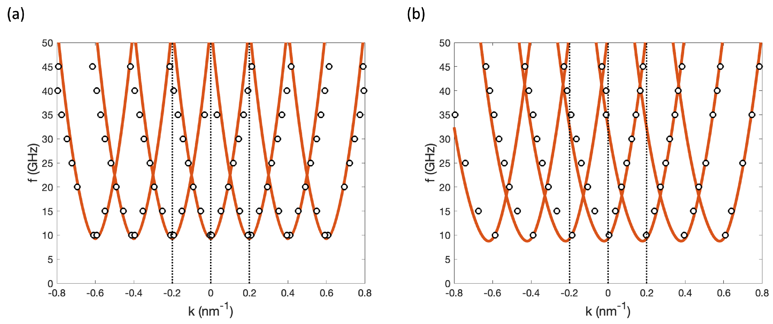
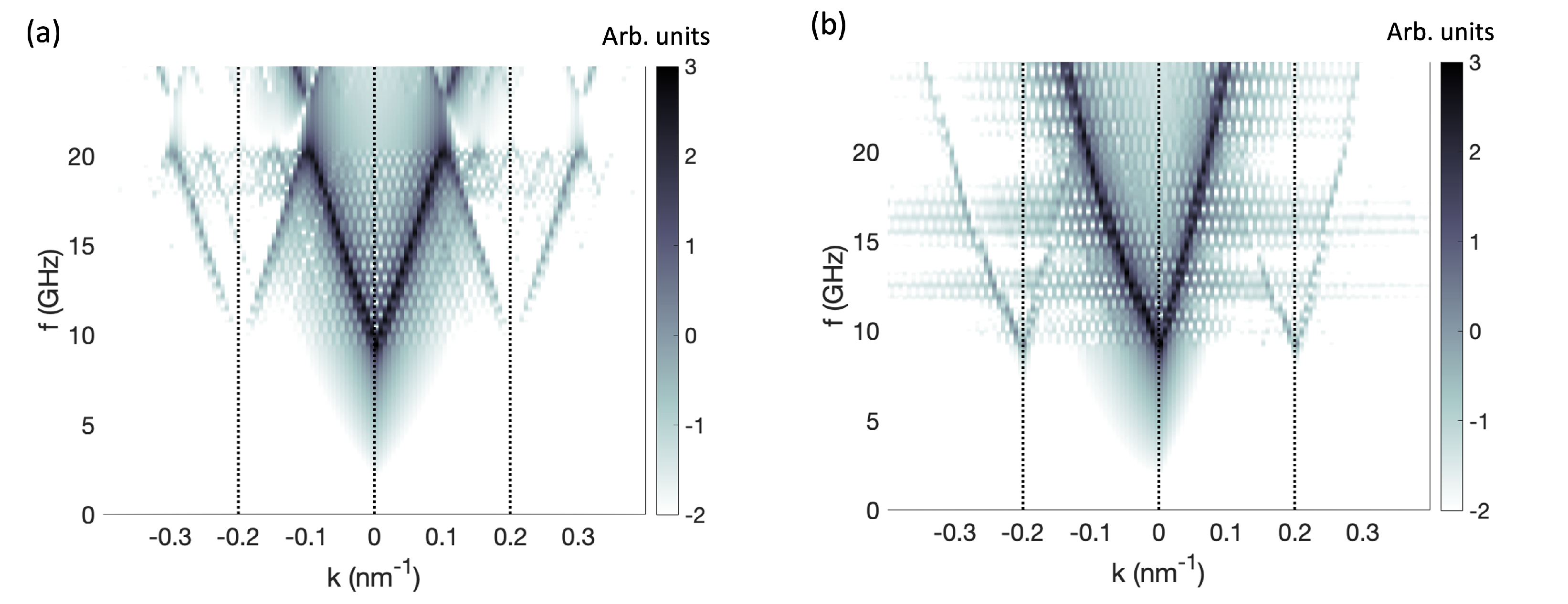
3.1. Dispersion Relations

The sinc pulse method described in Section 2.2.1 was used to numerically compute the dispersion relations. We used an external field of ${\mu }_0{\mathbf{H}}_0=0.1$ T in the y direction for the SW configuration and a field of ${\mu }_0{\mathbf{H}}_0=1.1$ T in z direction for the FVW configuration. Note that this field was slightly larger than the saturation magnetization, to ensure a uniform magnetized state normal to the film’s plane. Throughout these simulations, we used a modulation parameter $\beta =0.4$ to show the effect of the modulation.

We first simulated the variation in the exchange constant. The results are shown as a colorscale map in Figure 2. The FVW and SW configurations are shown in panels (a) and (b), respectively. The calculated dispersion relations are displayed using red curves. The solid curve was obtained with $N=0$, while the dotted curves were obtained with $N=\pm 1$. We found a reasonable qualitative agreement between the exchange-dominated dispersion and the numerical results. The main discrepancy was observed close to $k=0$, due to the nonlocal dipole field, which excited magnetostatic modes not included in our analytical calculations. In both cases, the bands interacted at the FBZ, $k=\pm 0.1$ nm⁻¹, leading to apparent bandgaps. The evanescent nature of the waves in between the bandgap in the SW configuration are shown in Section 3.1.1 These results demonstrate that the modulation of a continuous film can establish a band structure that is mediated by spin waves at the nanoscale.

Then, the DMI parameter was varied. We used $D=0.5$ mJ/m² as the average value, consistent with experimentally reported values for the interfacial DMI in CoFeB/Pt bilayers [45]. This is a relatively strong DMI interaction, but it is used here to showcase the effect of its spatial modulation. The numerical results are also displayed as colorscale maps in Figure 3, with panels (a) and (b) showing the FVW and SW configurations, respectively, and analytical calculations shown by red curves. In this case, we find more striking differences between the configurations. For the FVW configuration, we find only one dominant dispersion curve. This was expected from the analytical derivation, since DMI was not active in this case. However, some additional bands are visible. This was due to nonlinearities in the Landau–Lifshitz equation and can be considered negligibly small.

In the SW configuration, the simple exchange-dominated regime agreed remarkably well with the numerical right-propagating band. In addition, there is no apparent shift in the minimum of the dispersion relation, as was expected from the analytical calculations and the chirality induced by the DMI [43]. The reason for this was again the nonlocal dipole field. Because our modulation had a period of 32 nm, the magnetostatic waves were essentially impervious to the modification of DMI, and SW dominated the low-k dispersion. This implies that the DMI modulation at this scale does not result in a band structure, as otherwise observed for 1D magnonic crystals [34]. Instead, the effect of chirality for long-wave mangnons is completely suppressed, suggesting only a mean effect on the magnon nonreciprocity that can be otherwise expected from unpatterned ferromagnetic films grown on a heavy metal.

To verify that nonlocal dipole fields were indeed responsible for suppressing the DMI-induced minimum, we repeated the simulations by replacing the nonlocal dipole field with a local thin film approximation, i.e., a negative uniaxial anisotropy, such that $K_u=-{\mu }_0{M}_s^2/2$. The resulting dispersion relation shown in Figure 4 clearly exhibits a shifted parabolic behavior, as expected from Equation (7).

3.1.1. Local Microwave Field

To access higher frequencies in the dispersion relations, we used the local microwave field method. We focused on the SW configuration to establish at which point the analytical derivations agreed with the simulations with a nonlocal dipole field. We used microwave fields at frequencies ranging from 10 GHz to 45 GHz in steps of 5 GHz. For each of the eight simulations, we determined the right and left propagating wavenumbers. Because we had a band structure, there were multiple peaks for each frequency, which allowed us to probe $\left|N\right|>1$.

The results are shown in Figure 5 for modulations in exchange constant (a) and DMI constant (b) as black circles. The error in wavenumber was smaller than the circles in the figure. For the modulation in exchange, panel (a), we find a good agreement at frequencies under 25 GHz. At higher frequencies, the numerical results seem to exhibit a lower concavity. This may have been a consequence of the modulation parameter being too large and led to additional effects not captured by the small-wave approximation used in the analytical calculations. For the modulation in DMI shown in panel (b), a better agreement with the analytical calculations is found as the frequency increases, demonstrating that the magnetostatic waves had a negligible effect.

We note that in both cases, the reflected waves were neglected in the identification of wavenumbers. For this reason, only half of the bands were identified from the spectra.

This method could also be used to investigate the excitation of waves in between the apparent band gaps observed in Figure 2 for the case of exchange constant modulation. We used microwave fields around the band crossing at the FBZ as an example. We ran simulations for frequencies of 20 GHz, 21 GHz, 22 GHz, 23 GHz, and 24 GHz. To compare the excited waves, we ran a simulation for a time equal to 400 cycles of the microwave field. The spatial profiles of the $m_z$ component are shown in Figure 6. The waves were evanescent between 21 GHz and 23 GHz (solid gray curves), demonstrating the existence of a band gap of approximately 2 GHz. The waves at 20 GHz and 24 GHz (solid black curves) were propagating and extended past 1 μm, which is the typical decay length of waves in Py [46,47]. We also observed that there was a phase shift between the profile at 20 GHz and 24 GHz, which further suggested that the magnons pertained to different bands. In other words, for the same number of cycles, the spin wave at 20 GHz exhibited a maximum, while the spin wave at 24 GHz exhibited a minimum, away from the injection region.

3.2. Square Modulations

The TNL technique has, in principle, a spatial resolution of 10 nm. This means that it is possible to induce parameter modulations in more abrupt shapes. As a limiting test for the sharpness of such a parameter modulation, we investigated square modulations of both exchange and DMI parameters in the SW configuration.

From the Fourier properties, we expected square modulations to give rise to an increased number of harmonics. This modulation was defined on a continuous film, and thus we also expected each harmonic to be subject to the Bloch theorem, leading to an overall increase in spectral content. This expectation was consistent with the numerical simulations using the sinc method, as shown in Figure 7 for (a) exchange and (b) DMI square modulations. For this, we applied a sign function to the modulations described in Section 2.1. We emphasize that the same momentum and frequency resolution was maintained in this case, but the lack of imperfections led to well-defined harmonics. Experimentally, one would expect these harmonics to blur with defects and temperature, making the spectrum less defined and likely difficult to measure. Therefore, these simulations suggest that smoother modulations would be beneficial for defining nanoscale magnonic crystals. Naively, one would expect such a smooth modulation possible, given that a local annealing process would exhibit a thermal gradient.

Despite the increase in harmonics, it is important to note that the salient features of the spectra shown in Figure 2b and Figure 3b were maintained. Namely, a band gap was observed for the exchange constant modulation, while the DMI modulation was effectively suppressed.

Finally, we would like to note that such an increase in harmonics is typically not observed in magnonic crystals relying on nanopatterning [9,10,11,34]. This is both because magnetostatic waves are typically longer than the size of the patterned features and because the dipole field is a continuous vector field in free space. As a result, the coupling between elements is relatively smooth and the resulting band structure is well-defined.

4. Conclusions

We numerically investigated dispersion relations in thin films when magnetic parameters were modulated in space and at the nanoscale, a regime that is accessible using TNL [36]. We explored the modulation of the exchange and DMI constants. The former gave rise to band-gaps, while the latter was effectively suppressed by non-local dipole fields. The presented results suggest that nanoscale parameter modification is a viable route for defining magnonic crystals. Through local annealing, it should be possible to also modify the saturation magnetization and even uniaxial anisostropy, e.g., Co/Ni multilayers subject to surface imperfections. By locally modifying thin films into magnonic crystals, it might be possible to design controllable behavior and magnon interfaces, providing a foundation for magnonic devices accessing sub-100 nm wavelengths [48].

References

1. Balkanski, M.; Wallis, R. Semiconductor Physics and Applications; Oxford University Press: Oxford, UK, 2000. [Google Scholar]
2. Joannopoulos, J.D.; Johnson, S.G.; Winn, J.N.; Meade, R.D. Photonic Crystals: Molding the Flow of Light, 2nd ed.; Princeton University Press: Princeton, NJ, USA, 2008. [Google Scholar]
3. Kruglyak, V.V.; Demokritov, S.O.; Grundler, D. Magnonics. J. Phys. D Appl. Phys. 2010, 43, 264001. [Google Scholar] [CrossRef]
4. Grundler, D. Reconfigurable Magnonics Heats Up. Nat. Phys. 2015, 11, 438–441. [Google Scholar] [CrossRef]
5. Serga, A.A.; Chumak, A.V.; Hillebrands, B. YIG magnonics. J. Phys. D Appl. Phys. 2010, 43, 264002. [Google Scholar] [CrossRef]
6. Chumak, A.V.; Vasyuchka, V.I.; Serga, A.A.; Hillebrands, B. Magnon Spintronics. Nat. Phys. 2015, 11, 453–461. [Google Scholar] [CrossRef]
7. Barman, A.; Gubbiotti, G.; Ladak, S.; Adeyeye, A.O.; Krawczyk, M.; GrÄfe, J.; Adelmann, C.; Cotofana, S.; Naeemi, A.; Vasyuchka, V.I.; et al. The 2021 Magnonics Roadmap. J. Phys. Condens. Matter. 2021, 33, 413001. [Google Scholar] [CrossRef]
8. Chumak, A.V.; Kabos, P.; Wu, M.; Abert, C.; Adelmann, C.; Adeyeye, A.O.; Åkerman, J.; Aliev, F.G.; Anane, A.; Awad, A.; et al. Advances in Magnetics Roadmap on Spin-Wave Computing. IEEE Trans. Magn. 2022, 58, 1–72. [Google Scholar] [CrossRef]
9. Nikitov, S.; Tailhades, P.; Tsai, C. Spin Waves in Periodic Magnetic Structures-Magnonic Crystals. J. Magn. Magn. Mater. 2001, 236, 320–330. [Google Scholar] [CrossRef]
10. Wang, Z.K.; Zhang, V.L.; Lim, H.S.; Ng, S.C.; Kuok, M.H.; Jain, S.; Adeyeye, A.O. Observation of frequency band gaps in a one-dimensional nanostructured magnonic crystal. Appl. Phys. Lett. 2009, 94, 083112. [Google Scholar] [CrossRef]
11. Wang, Z.; Zhang, V.; Lim, H.; Ng, S.; Kuok, M.; Jain, S.; Adeyeye, A. Nanostructured magnonic crystals with size-tunable bandgaps. ACS Nano 2010, 4, 643–648. [Google Scholar] [CrossRef] [PubMed]
12. Frey, P.; Nikitin, A.A.; Bozhko, D.A.; Bunyaev, S.A.; Kakazeri, G.N.; Ustinov, A.B.; Kalinikos, B.A.; Ciubotaru, F.; Chumak, A.V.; Wang, Q.; et al. Reflection-less width-modulated magnonic crystal. Npj Commun. Phys. 2020, 3, 17. [Google Scholar] [CrossRef]
13. Krawczyk, M.; Puszkarski, H. Plane-wave theory of three-dimensional magnonic crystals. Phys. Rev. B 2008, 77, 054437. [Google Scholar] [CrossRef]
14. Tacchi, S.; Montoncello, F.; Madami, M.; Gubbiotti, G.; Carlotti, G.; Giovannini, L.; Zivieri, R.; Nizzoli, F.; Jain, S.; Adeyeye, A.O.; et al. Band Diagram of Spin Waves in a Two-Dimensional Magnonic Crystal. Phys. Rev. Lett. 2011, 107, 127204. [Google Scholar] [CrossRef]
15. Zivieri, R.; Montoncello, F.; Giovannini, L.; Nizzoli, F.; Tacchi, S.; Madami, M.; Gubbiotti, G.; Carlotti, G.; Adeyeye, A.O. Collective spin modes in chains of dipolarly interacting rectangular magnetic dots. Phys. Rev. B 2011, 83, 054431. [Google Scholar] [CrossRef]
16. Kumar, D.; Kłos, J.W.; Krawczyk, M.; Barman, A. Magnonic band structure, complete bandgap, and collective spin wave excitation in nanoscale two-dimensional magnonic crystals. J. Appl. Phys. 2014, 115, 043917. [Google Scholar] [CrossRef]
17. Tacchi, S.; Gubbiotti, G.; Madami, M.; Carlotti, G. Brillouin light scattering studies of 2D magnonic crystals. J. Phys. Condens. Matter. 2017, 29, 073001. [Google Scholar] [CrossRef] [PubMed]
18. Skjærvø, S.H.; Marrows, C.H.; Stamps, R.L.; Heyderman, L.J. Advances in artificial spin ice. Nat. Rev. Phys. 2020, 2, 13–28. [Google Scholar] [CrossRef]
19. Gliga, S.; Kákay, A.; Hertel, R.; Heinonen, O.G. Spectral Analysis of Topological Defects in an Artificial Spin-Ice Lattice. Phys. Rev. Lett. 2013, 110, 117205. [Google Scholar] [CrossRef]
20. Iacocca, E.; Gliga, S.; Stamps, R.L.; Heinonen, O. Reconfigurable Wave Band Structure of an Artificial Square Ice. Phys. Rev. B 2016, 93, 134420. [Google Scholar] [CrossRef]
21. Jungfleisch, M.B.; Zhang, W.; Iacocca, E.; Sklenar, J.; Ding, J.; Jiang, W.; Zhang, S.; Pearson, J.E.; Novosad, V.; Ketterson, J.B.; et al. Dynamic Response of an Artificial Square Spin Ice. Phys. Rev. B 2016, 93, 100401. [Google Scholar] [CrossRef]
22. Iacocca, E.; Heinonen, O. Topologically Nontrivial Magnon Bands in Artificial Square Spin Ices with Dzyaloshinskii-Moriya Interaction. Phys. Rev. Appl. 2017, 8, 034015. [Google Scholar] [CrossRef]
23. Iacocca, E.; Gliga, S.; Heinonen, O.G. Tailoring Spin-Wave Channels in a Reconfigurable Artificial Spin Ice. Phys. Rev. Appl. 2020, 13, 044047. [Google Scholar] [CrossRef]
24. Gliga, S.; Iacocca, E.; Heinonen, O.G. Dynamics of reconfigurable artificial spin ice: Toward magnonic functional materials. APL Mater. 2020, 8, 040911. [Google Scholar] [CrossRef]
25. Negrello, R.; Montoncello, F.; Kaffash, M.T.; Jungfleisch, M.B.; Gubbiotti, G. Dynamic coupling and spin-wave dispersions in a magnetic hybrid system made of an artificial spin-ice structure and an extended NiFe underlayer. APL Mater. 2022, 10, 091115. [Google Scholar] [CrossRef]
26. Lendinez, S.; Kaffash, M.T.; Heinonen, O.G.; Gliga, S.; Iacocca, E.; Jungfleisch, M.B. Nonlinear multi-magnon scattering in artificial spin ice. Nat. Commun. 2023, 14, 3419. [Google Scholar] [CrossRef] [PubMed]
27. Heyderman, L.J.; Stamps, R.L. Artificial Ferroic Systems: Novel Functionality from Structure, Interactions and Dynamics. J. Phys. Condens. Matter. 2013, 25, 363201. [Google Scholar] [CrossRef] [PubMed]
28. Lendinez, S.; Jungfleisch, M.B. Magnetization dynamics in artificial spin ice. J. Phys. Condens. Matter. 2019, 32, 013001. [Google Scholar] [CrossRef] [PubMed]
29. Arroo, D.M.; Gartside, J.C.; Branford, W.R. Sculpting the spin-wave response of artificial spin ice via microstate selection. Phys. Rev. B 2019, 100, 214425. [Google Scholar] [CrossRef]
30. Bhat, V.S.; Watanabe, S.; Baumgaertl, K.; Kleibert, A.; Schoen, M.A.W.; Vaz, C.A.F.; Grundler, D. Magnon Modes of Microstates and Microwave-Induced Avalanche in Kagome Artificial Spin Ice with Topological Defects. Phys. Rev. Lett. 2020, 125, 117208. [Google Scholar] [CrossRef] [PubMed]
31. Caravelli, F.; Nisoli, C. Logical gates embedding in artificial spin ice. New J. Phys. 2020, 22, 103052. [Google Scholar] [CrossRef]
32. Kaffash, M.T.; Lendinez, S.; Jungfleisch, M.B. Nanomagnonics with artificial spin ice. Phys. Lett. A 2021, 402, 127364. [Google Scholar] [CrossRef]
33. Gartside, J.C.; Stenning, K.D.; Vanstone, A.; Holder, H.H.; Arroo, D.M.; Dion, T.; Caravelli, F.; Kurebayashi, H.; Branford, W.R. Reconfigurable training and reservoir computing in an artificial spin-vortex ice via spin-wave fingerprinting. Nat. Nanotechnol. 2022, 17, 460–469. [Google Scholar] [CrossRef]
34. Gallardo, R.A.; Cortés-Ortuño, D.; Schneider, T.; Roldán-Molina, A.; Ma, F.; Troncoso, R.E.; Lenz, K.; Fangohr, H.; Lindner, J.; Landeros, P. Flat Bands, Indirect Gaps, and Unconventional Spin-Wave Behavior Induced by a Periodic Dzyaloshinskii-Moriya Interaction. Phys. Rev. Lett. 2019, 122, 067204. [Google Scholar] [CrossRef]
35. Albisetti, E.; Petti, D.; Pancaldi, M.; Madami, M.; Tacchi, S.; Curtis, J.; King, W.P.; Papp, A.; Csaba, G.; Porod, W.; et al. Nanopatterning reconfigurable magnetic landscapes via thermally assisted scanning probe lithography. Nat. Nanotechnol. 2016, 11, 545–551. [Google Scholar] [CrossRef]
36. Levati, V.; Girardi, D.; Pellizzi, N.; Panzeri, M.; Vitali, M.; Petti, D.; Albisetti, E. Phase Nanoengineering via Thermal Scanning Probe Lithography and Direct Laser Writing. Adv. Mater. Technol. 2023, 8, 2300166. [Google Scholar] [CrossRef]
37. Auric, P.; Bouat, S.; Rodmacq, B. Structural and magnetic properties of annealed multilayers studied by Mössbauer spectroscopy, X-ray diffraction and magnetization measurements. J. Phys. Condens. Matter. 1998, 10, 3755. [Google Scholar] [CrossRef]
38. Yin, Y.; Pan, F.; Ahlberg, M.; Ranjbar, M.; Dürrenfeld, P.; Houshang, A.; Haidar, M.; Bergqvist, L.; Zhai, Y.; Dumas, R.K.; et al. Tunable permalloy-based films for magnonic devices. Phys. Rev. B 2015, 92, 024427. [Google Scholar] [CrossRef]
39. Khan, R.A.; Shepley, P.M.; Hrabec, A.; Wells, A.W.J.; Ocker, B.; Marrows, C.H.; Moore, T.A. Effect of annealing on the interfacial Dzyaloshinskii-Moriya interaction in Ta/CoFeB/MgO trilayers. Appl. Phys. Lett. 2016, 109, 132404. [Google Scholar] [CrossRef]
40. Vansteenkiste, A.; Leliaert, J.; Dvornik, M.; Helsen, M.; Garcia-Sanchez, F.; Van Waeyenberge, B. The Design and Verification of MuMax3. AIP Adv. 2014, 4, 107133. [Google Scholar] [CrossRef]
41. Sprenger, P.; Hoefer, M.A.; Iacocca, E. Magnonic Band Structure Established by Chiral Spin-Density Waves in Thin-Film Ferromagnets. IEEE Magn. Lett. 2019, 10, 4501605. [Google Scholar] [CrossRef]
42. Szulc, K.; Tacchi, S.; Hierro-Rogríguez, A.; Díaz, J.; Gruszecki, P.; Graczyk, P.; Quirós, C.; Markó, D.; Martín, J.I.; Vélez, M.; et al. Reconfigurable Magnonic Crystals Based on Imprinted Magnetization Textures in Hard and Soft Dipolar-Coupled Bilayers. ACS Nano 2022, 16, 14168–14177. [Google Scholar] [CrossRef] [PubMed]
43. Nembach, H.T.; Shaw, J.M.; Weiler, M.; Jué, E.; Silva, T.J. Linear relation between Heisenberg exchange and interfacial Dzyaloshinskii-Moriya Interaction in metal films. Nat. Phys. 2015, 11, 825. [Google Scholar] [CrossRef]
44. Venkat, G.; Kumar, D.; Franchin, M.; Dmytriiev, O.; Mruczkiewicz, M.; Fangohr, H.; Barman, A.; Krawczyk, M.; Prabhakar, A. Proposal for a standard micromagnetic problem: Spin wave dispersion in a magnonic waveguide. IEEE Trans. Magn. 2013, 49, 524. [Google Scholar] [CrossRef]
45. Tacchi, S.; Troncoso, R.E.; Ahlberg, M.; Gubbiotti, G.; Madami, M.; Åkerman, J.; Landeros, P. Interfacial Dzyaloshinskii-Moriya Interaction in Pt/CoFeB Films: Effect of the Heavy-Metal Thickness. Phys. Rev. Lett. 2017, 118, 147201. [Google Scholar] [CrossRef] [PubMed]
46. Madami, M.; Bonetti, S.; Consolo, G.; Tacchi, S.; Carlotti, G.; Gubbiotti, G.; Mancoff, F.B.; Yar, M.A.; Åkerman, J. Direct observation of a propagating spin wave induced by spin-transfer torque. Nat. Nanotechnol. 2011, 6, 635–638. [Google Scholar] [CrossRef]
47. Madami, M.; Iacocca, E.; Sani, S.; Gubbiotti, G.; Tacchi, S.; Dumas, R.K.; Åkerman, J.; Carlotti, G. Propagating spin waves excited by spin-transfer torque: A combined electrical and optical study. Phys. Rev. B 2015, 92, 024403. [Google Scholar] [CrossRef]
48. Yu, H.; Duerr, G.; Huber, R.; Bahr, M.; Schwarze, T.; Brandl, F.; Grundler, D. Omnidirectional Spin-Wave Nanograting Coupler. Nat. Commun. 2013, 4, 2702. [Google Scholar] [CrossRef]
Figure 1. Schematic illustration of the investigated configurations. The gradient red regions display the periodicity of the magnetic parameters with wavenumber q. The magnons propagated along the modulated parameters with wavenumber k. The (a) forward volume wave (FWV) and (b) surface wave (SW) configurations were achieved by using a saturating magnetic field normal to the plane and a small magnetic field in-plane and perpendicular to k, respectively.
Magnetochemistry 10 00014 g001
Figure 2. Numerical dispersion relations when the exchange constant is modulated with β = 0.4 and q = 0.2 nm−1 for (a) FVW and (b) SW configurations. The analytical equations from Equations (3) and (4) are superimposed with red curves. The solid curve was calculated with N = 0 , and the dashed curves were computed with N = ± 1 . The black dashed lines at k = 0.2 and 0.2 nm−1 represent the modulation period. The semi-transparent region in (b) displays the frequency gap.
Magnetochemistry 10 00014 g002
Figure 3. Numerical dispersion relations when the DMI constant was modulated with β = 0.4 and q = 0.2 nm−1 for the (a) FVW and (b) SW configurations. The analytical equations from Equations (3) and (4) are superimposed with red curves. The solid curve was calculated with N = 0 , and the dashed curves were computed with N = ± 1 . The black dashed lines at k = 0.2 and 0.2 nm−1 represent the modulation period.
Magnetochemistry 10 00014 g003
Figure 4. Numerical dispersion relations for the SW configuration when the DMI constant was modulated with β = 0.4 and q = 0.2 nm−1. The non-local dipole contribution was removed from these simulations and replaced by a negative uniaxial anisotropy that mimicked the thin film approximation used in the analytical calculations. Because the magnetostatic waves were not available, the derived dispersions accurately predicted the numerical results. The black dashed lines at k = 0.2 and 0.2 nm−1 represent the modulation period.
Magnetochemistry 10 00014 g004
Figure 5. Numerically determined wavenumber values for a range of microwave frequencies, shown by black circles. These are compared with analytical calculations shown in solid red curves with modulations in the (a) exchange constant and (b) the DMI constant. The black dashed lines at k = 0.2 and 0.2 nm−1 represent the modulation period.
Magnetochemistry 10 00014 g005
Figure 6. Wave profiles from the m z component excited by a microwave field. The solid black curves are propagating waves, while the solid gray curves are evanescent waves. The simulations were run for 400 microwave cycles to ensure the same phase was obtained. The profiles are vertically shifted for clarity.
Magnetochemistry 10 00014 g006
Figure 7. Numerical dispersion relations in the SW configuration using a square modulation of (a) exchange and (b) DMI parameters. The dispersion relations had an increased spectral content because of the harmonics enabled by the square modulation. The black dashed lines at k = 0.2 and 0.2 nm−1 represent the modulation period.
Magnetochemistry 10 00014 g007
Disclaimer/Publisher’s Note: The statements, opinions and data contained in all publications are solely those of the individual author(s) and contributor(s) and not of MDPI and/or the editor(s). MDPI and/or the editor(s) disclaim responsibility for any injury to people or property resulting from any ideas, methods, instructions or products referred to in the content.