Article

Research on Mixing Law of Liquid Fertilizer Injected into Irrigation Pipe

Research Center of Fluid Machinery and Technology, Jiangsu University, Zhenjiang 212013, China
*
Author to whom correspondence should be addressed.
Horticulturae 2022, 8(3), 200; https://doi.org/10.3390/horticulturae8030200
Submission received: 11 January 2022 / Revised: 15 February 2022 / Accepted: 22 February 2022 / Published: 24 February 2022
(This article belongs to the Special Issue Advanced of Horticulture Innovative Irrigation Technologies)

Abstract

:
The time and position that fertilizer takes to uniformly mix with water in an irrigation system significantly affects the development of a fertilization strategy. A pipe irrigation system was used to study the fertilizer–water mixing law in irrigation pipes using numerical simulation and experiments. The effect of the diameter of the water pipe and fertilizer pipe, water and fertilizer flow rates, concentration and viscosity of fertilizer, frequency of fertilizer injection on the mixing speed, and uniform mixing length indicated that the frequency of fertilizer injection did not affect the mixing process. The increase in the water pipe diameter and fertilizer flow rate or the decrease in fertilizer pipe and water flow rate diameter result in the increase of the speed of fertilizer solution mixing with water along the radial direction of the mixing pipe. The uniform mixing length was directly proportional to the fertilizer pipe diameter, water pipe diameter, water flow rate, and fertilizer viscosity, while it was inversely proportional to the flow rate and concentration of fertilizer. The relationship between the uniform mixing length and six influencing factors was fitted, the fitting was highly accurate, and the fitting equation can be used to predict the uniform mixing length under other conditions.

1. Introduction

Fertigation is an efficient fertilization technology that can improve fertilizer efficiency and reduce the amount of fertilizer applied, thus reducing the amount of pollution caused by excessive fertilization [1,2]. Water soluble fertilizer enters the irrigation system through fertilization equipment, mixes with water, and is then finally transported to the field. Ideally, the fertilizer and water should mix uniformly before the solution is discharged. Thus, it is necessary to investigate the mixing law of water and fertilizer in the irrigation system. Pipe irrigation is a widely used irrigation system in agricultural fertigation, and the research on fertilizer–water mixing in pipes can easily be realized under laboratory conditions and can provide a reference for the study of water–fertilizer mixing in other irrigation systems such as canal and drip irrigation.
Fertilizer–water mixing in the pipes is essentially liquid–liquid mixing, which is caused by convection and molecular diffusion [3]. A substantial amount of experimental research on liquid–liquid mixing in pipes has been conducted. To visualize the liquid–liquid mixing in the pipeline, the experimental pipes are usually transparent, and many methods have been adopted to measure the distribution of solutes in the solvent liquid. A simple way is to dye the solute liquid and then compare the color pixel of every point in the pipe [4]. A more accurate approach is to add photoactivatable fluorophores into the solute liquid and then use particle image velocimetry (PIV) and planer laser induced fluorescence (PLIF) to measure the liquid distribution after the two liquids had merged [5]. Many factors that affect the mixing process have been considered in experiments. Ger et al. [6] investigated the influence of three jet modes (a center line source, a wall source, and a jet at the wall issuing perpendicularly) on mixing, and found that the mixing took place most rapidly when the liquid was injected by the central line source. Nakayama et al. [7] proposed that the flow ratio of the two inlets had a significant effect on the mixing speed, and the mixing degree of the two liquids was more thorough as the distance increased. Han et al. [4] found that the difference in viscosity between the two liquids would affect the mixing speed. Hansen et al. [5] indicated that a small change in the inlet geometry would have a substantial influence on the mixing rate. Mi et al. [8] conducted experiments at the Fluid-Structure-Interaction test facility to explore the mixing state of hot and cold water near T-joints when the T-junction had a weld inside the pipe. In these experiments, liquid was injected into the pipe at a constant flow rate, but for many sprinkler pipe systems, the fertilizer was pulse injected by a plunger pump or diaphragm pump [9,10]. There was little research on the mixing process of the liquid pulse injected into the pipe.
Although advanced experimental methods and equipment enable successful research on liquid–liquid mixing in pipes, the experiment was very expensive. In addition, due to the shielding of the outer solution, it was difficult to completely observe the distribution of solutes in the pipeline. Thus, the content of distribution of the solute distribution in the pipe was calculated using a numerical method. With the development of computer computing analysis technology, numerical simulation software has been used to solve more complex numerical models such as to research the liquid–liquid mixing process in pipes. Zughbi [11] conducted numerical and experimental investigations on the mixing of hot and cold water in the pipe. They measured the mixing uniformity by the temperature distribution on the pipe section and delineated that the pipe length required to achieve 95% mixing was related to the ratio of flow rate of the main and side pipes. Lateef et al. [12] built a two-dimensional pipe model and simulated the flow state in the pipeline and the mixing velocity of solutes in water using Comsol Multiphysics software. They found that the increase in water velocity could accelerate the mixing of solutes and water in the pipe. Lin et al. [13] adopted several steady-state turbulence models in CFD software to simulate the thermal mixing in the T-pipe and found that the simulated results in the k–ε turbulence model were the most consistent with the experimental results. Sun et al. [14] adopted a mixture model to simulate the water–saline mixing in the pipe and investigated the influence of pipe size, flow ratio, and Reynolds number on the mixing uniformity. In most studies, the two liquids were considered to be two phases, and a multinomial flow model was used to calculate the material exchange between the solute and solvent liquids. However, water and liquid fertilizer are mutually soluble in-phase liquids, and the simulation of water fertilizer mixing with a multiphase flow model will substantially deviate from the actual situation.
To investigate the water–fertilizer mixing law in pipes, a CFD simulation method based on the species transport model was proposed, and experiments were conducted to validate the feasibility of the simulation results. Factors that may affect the mixing law were considered in the simulation. Based on the experimental and simulation results, the influence of each factor on the mixing speed and uniformity mixing length was obtained. The relationship between the uniformity mixing length and each factor was established, and it can be used to predict the uniformity mixing length under other working conditions.

2. Materials and Methods

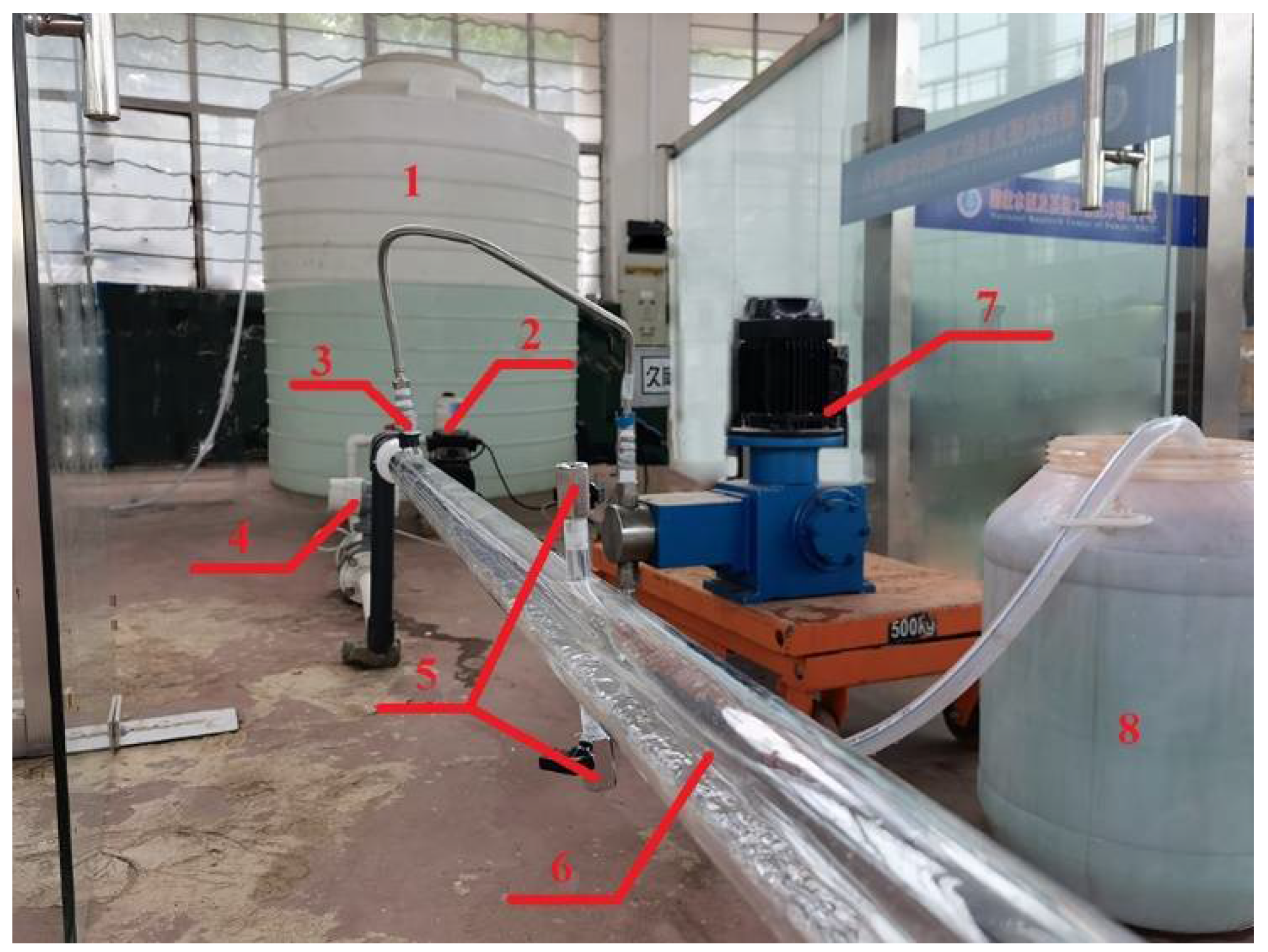
2.1. Experimental Establishment

Experiments were conducted to explore the water–fertilizer mixing law in the irrigation pipe after the fertilizer solution was injected into the pipeline and investigate the effect of pipeline structure parameters, hydraulic parameters, and fertilizer physical properties on the mixing uniformity. The pipeline structure parameters included the water pipe diameter (D) and fertilizer pipe diameter (d). The hydraulic parameters consisted of the water flow rate (Q), fertilizer flow rate (q), and fertilizer injection frequency (f). The fertilizer physical properties included the fertilizer concentration (C) and fertilizer viscosity (η). The experimental equipment site is shown in Figure 1. A water tank with a volume of 5 m3 was adopted as the water source. The centrifugal pump (CM5-6, Grundfos, Denmark) and flowmeter (CKLDG/LDG, China, accuracy of ±0.5%) were used to supply water to the pipe system and display the water flow rate. Fertilizer was injected into the pipe system using a plunger pump (WEILI, China, maximum flow rate of 0.3 m3h−1). Considering the practical engineering application, the pipe was produced by polyethylene materials. To master the fertilizer distribution law in the pipe, 20 sampling pipes with ball values were fixed in the upper and lower sections of the straight pipe. The arrangement of sampling points is shown in Figure 2. The center line of the thin standpipe, which was set for injecting fertilizer solution, was established as Y0. Sampling positions were then arranged every 1 m from the Y0 position. Two sampling pipes that were 6 mm in diameter and length of 40 mm long were established at the upper and lower areas of the sampling position.
Fertilizer injected into the pipeline is usually a solution of water and solid fertilizer, with viscosity possibly related to the type and concentration of the fertilizer. Accordingly, the viscosity of the different fertilizer solutions with multiple concentrations was tested before the mixing experiment. The solid fertilizers included compound fertilizer (N + P2O + K2O ≥ 40%, N18: P12: K12) and potassium chloride (K2O ≥ 60%), and the viscosity was tested using a viscometer (NDJ-1, LICHEN, Shanghai, China). The results are shown in Table 1. The viscosity of the fertilizer concentration was found be unrelated to the concentration. Averaging the data in Table 1, the viscosity of two types of solid fertilizer aqueous solutions (compound fertilizer and potassium chloride) were 0.0022 and 0.0055 kgm−1s−1, respectively.
Based on the experimental equipment parameters and fertilizer properties, full factor experiments were conducted to investigate the mixing law in pipes. The experimental design is shown in Table 2. In practice, fertilization was conducted during the process of irrigation, and water was supplied to fill the pipe in the initial 5 min of the experiment. Fertilizer was then injected to the pipe system until the end of the experiment. The samplings were conducted after 2 min of fertilizer injection to ensure the fertilizer mixed well with water in the pipe system. The first sampling was conducted at the two pipes of position Y1, and samplings were conducted at the next sampling position every minute. Conductivities of 20 samples were measured using a conductivity meter (CT-3031, JINCHE, China) and then converted to concentration. The relationship between the concentration and conductivity of two fertilizers were tested before the mixing experiment and the linear relationship [15,16] are shown in Figure 3.
After fertilizer was injected into the irrigation pipe, it would mix with water and finally be uniformly distributed on the radial section of the pipe. To study the axial position that fertilizer and water are uniformly mixed in the pipe, the coefficient of variation method [17] was adopted. When the COV value was <0.01, the fertilizer had uniformly mixed with the water.
C O V = 1 n i = 1 n ( C i C ¯ ) 2 C ¯
where n is the number of sampling points on the radial section and Ci and C ¯ denote the fertilizer concentration at the i-th sampling points on the radial section and the average value of concentration of all samplings, respectively. The distance from the Y0 position was established to be the mixing distance. The mixing distance was where the COV value of <0.01 was established as the uniform mixing length (Lu). There were 128 groups of full factor experiments to be conducted, and various models of pipelines, centrifugal pumps, and plunger pumps were required to satisfy the experimental design, which led to the extremely high cost of the experiment. In addition, the concentration on the radial section was difficult to directly measure in the experiment. Therefore, a numerical simulation was considered to study the fertilizer–water mixing law. Four groups of experiments (D1d1Q1q1C1η1f1, D1d1Q1q1C1η2f1, D1d1Q1q1C2η1f1, and D1d1Q1q1C2η2f1) were conducted to verify the simulation results because the changes in concentration and viscosity of fertilizers are inexpensive and convenient to use in the experiments.

2.2. Computational Fluid Dynamics Simulation

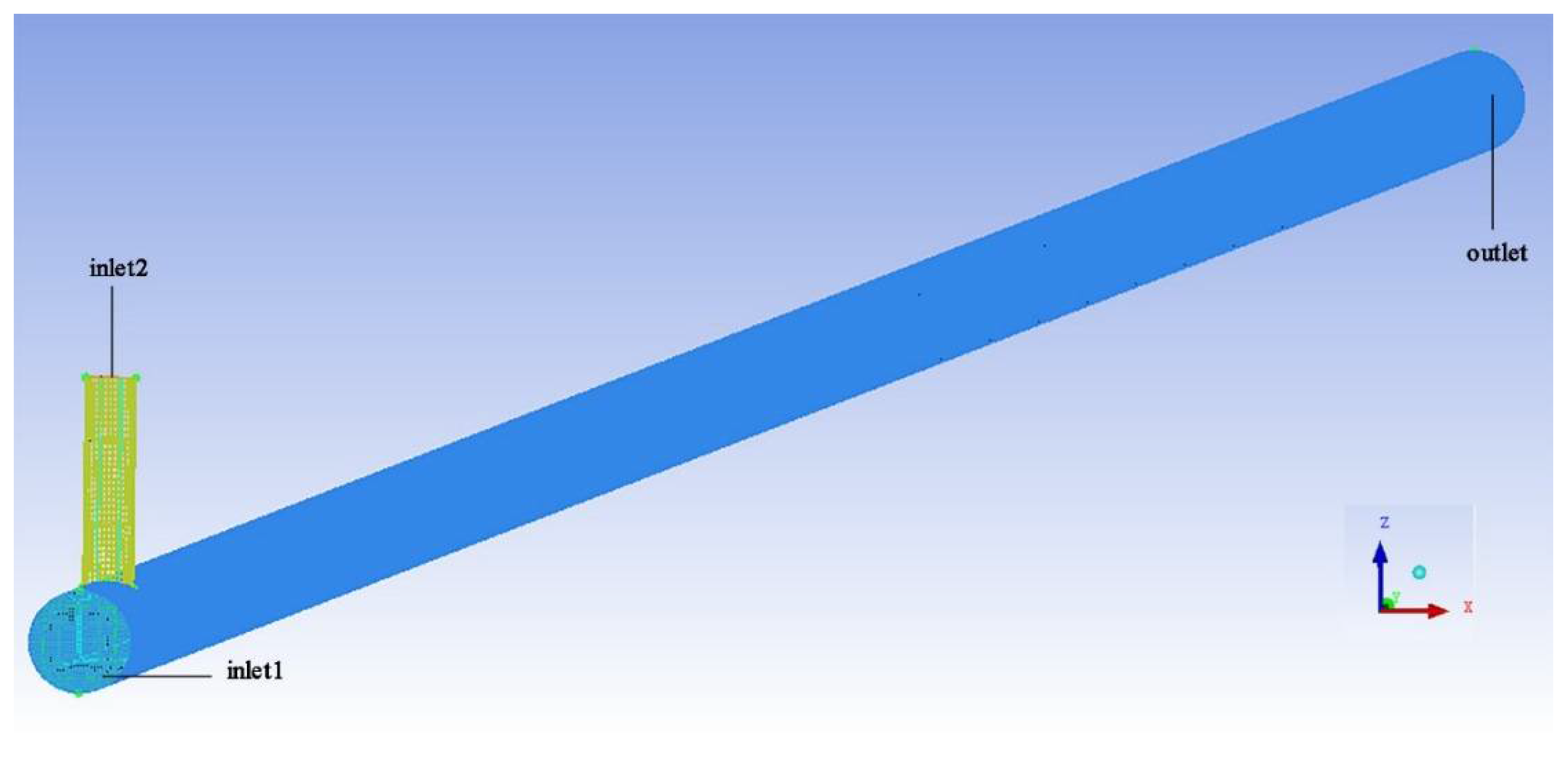
2.2.1. The Geometric Model

The geometric model shown in Figure 4 was conducted to simulate the mixing process. The proposed model consisted of a long straight pipe that was 10 m long and a thin standpipe that was 0.1 m long. The standpipe was 0.2 m away from inlet1. Water flowed into the straight pipe from inlet1; fertilizer was injected from inlet2, and the solution was discharged from the outlet.
Based on the geometric model and pipe parameters shown in Table 2, numerical models of the inner flow channel of the mixing pipeline were constructed in the ICEM module of Ansys software (version of 17.0, ANSYS, America). Hexahedral meshes were used to construct the numerical model, and boundary layer meshes were refined to improve the accuracy of simulation. One of the numerical models (D1d1) is shown in Figure 5. The diameter of inlet1 and inlet2 were 0.050 and 0.025 m, respectively, and the total number of cells was 2,432,007.

2.2.2. Governing Equation

The numerical models constructed were imported to the Fluent module of Ansys software, which is widely used in the field of fluid simulation. The flow state in the straight pipe and standpipe were all turbulent. Thus, the turbulence model was adapted in the simulation. The gravity in the Z direction was considered, and the gravitational acceleration was −9.81 ms−2. The standard k–ε, turbulence model [18,19] was chosen, and the near wall treatment was the standard wall functions. The fertilizer that was injected into the pipe was the solution of water and water-soluble solid fertilizer. It could be miscible with water in any proportion. The viscous liquid models adopted the species transport model [20,21], which was widely used to solve the problem of molecular exchange between two substances. The continuity equation was as follows:
t ( k = 1 n α k ρ k ) + ( k = 1 n α k ρ k v k ) = 0
where k is the number of the species in the models, and αk (%), ρk (kgm−3), and vk (ms−1) denote the volume fraction, density, and average velocity of the k species, respectively. The momentum equation was expressed as Equation (3):
t ( k = 1 n α k ρ k v k ) + ( k = 1 n α k ρ k v k v k ) = α k p + [ α k ( τ k + τ k t ) ] + α k ρ k g + F
where p (Pa) is the pressure; τk (Nm−2) and τkt (Nm−2) denote molecule momentum and turbulent stress; g (ms−2) is the acceleration of gravity; and F (Nm−3) signifies the volume force. The energy equation was developed as follows:
t ( k = 1 n α k ρ k h k ) + [ k = 1 n α k v k ( ρ k h k + p ) ] = k e f f ( T ) ,
where hk, keff, and T denote the sensible enthalpy of k species, effective thermal conductivity, and temperature, respectively. Moreover, according to the conservation law of components, the mass conservation equation of k species can be obtained from Equation (5):
( ρ k α k ) t + ( ρ k v k α k ) = [ D k × ( ρ k α k ) ]
where Dk is the diffusion coefficient.

2.2.3. Boundary Conditions

The density and viscosity of fluid materials will affect the efficiency of mixing. The fluid materials filled in the numerical models were a solution of water and fertilizer. Inlet1 and inlet2 both selected the velocity­inlet, and the outlet was designed based on the pressure-outlet. The fertilizer was injected into the thin standpipe in pulse form by a plunger pump. The flow rate of the fertilizer was as follows:
q i n s = q [ 1 + c o s ( 2 π f t ) ]
where qins (m3h−1) is the instantaneous flow rate of fertilizer, and t (s) is the time. The velocity magnitude of inlet1 and inlet2 were related to the flow rate of water and fertilizer, which are shown in the following equations:
v 1 = 4 Q / π D 2
v 2 = 4 q i n s / π d 2 = 4 q [ 1 + c o s ( 2 π f t ) ] π d 2
where v1 and v2 (ms−1) are the velocity magnitude of boundary conditions in inlet1 and inlet2. The turbulent intensity was established as 5%, and the hydraulic diameter was related to the size of inlet1, inlet2, and the outlet. The scheme of pressure-velocity coupling was SIMPLE. The spatial discretization was established as follows: the least squares cell based was chosen for gradient; the body force weighted was selected for pressure; the first order upwind was employed for turbulent kinetic energy, turbulent dissipation rate, and the second order upwind was used for momentum, species, and energy. The first order implicit was selected for transient formulation. The initialization methods chose standard initialization, and the initial water mass fraction was established as 1. The time step was established as 0.003 s, and the iterations were 5000.

2.3. Mesh Independence Check

Taking D1d1Q1q1C1η1f1 conditions as an example, three sizes of mesh were selected to partition the numerical model, and the total number of cells were 2,432,007, 2,916,157, and 3,648,932. The mesh independence was checked by comparing the fertilizer mass fraction in position Y1 and Y2 using the same boundary condition. Table 3 shows that the fertilizer mass fractions were almost identical at the same positions in three groups of simulation. Therefore, the mesh size of 2,432,007 cells was chosen to reduce the simulation time.

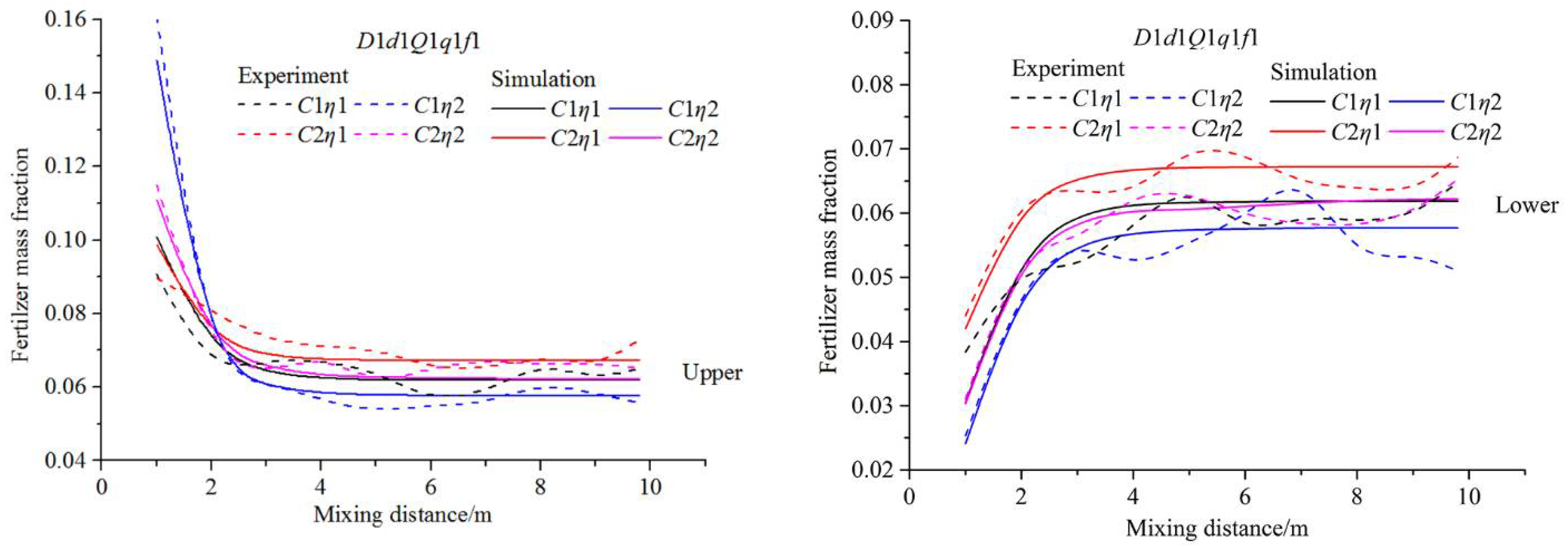
2.4. Comparison of Numerical and Experimental Results

The conductivity of samples was the direct measurement of data in the experimental results, while the directly observed data in the simulation results were the mass fraction of fertilizer species. To compare the simulation and experimental results, it was necessary to transfer fertilizer concentrations to fertilizer mass fractions. It was assumed that the fertilizer with a concentration of Cin (gL−1) and a volume of 1 L was mixed with water of V1 L, the density of the fertilizer was ρ1. The concentration of the mixture (C) would be as follows:
C = C i n 1 1 + V 1 = C i n 1 + V 1
In this research, the fertilizer solution was obtained by mixing solid fertilizer and water, and the amount of fertilizer was far less than that of water. Therefore, the increase in the volume of solution caused by dissolving can be negligible. Thus, Equation (10) can be obtained:
ρ 1 = C i n i t i a l 1 + ρ w 1 1 = C i n + ρ w = C i n + 1000
where ρw is the density of water. The fertilizer mass fraction of the mixture would be as follows:
ω = ρ 1 1 ρ 1 1 + ρ w V 1 = C i n + 1000 C i n + 1000 + 1000 V 1
where ω is the fertilizer mass fraction of the samplings. Equation (12) was obtained based on Equation (9):
V 1 = C i n C 1
Substituting Equation (12) into (11), the relationship between the fertilizer mass fraction and concentration can be obtained from Equation (13).
ω = C ( C i n + 1000 ) C i n ( C + 1000 )
The experimental data were transferred to the fertilizer mass fraction. The fertilizer mass fraction at the same position as the experimental sampling point in the simulation results were collected and drawn in Figure 6. The variation trend of the fertilizer mass fraction along the mixing distance in the simulation result was almost identical with that in the experimental results in all four cases. As shown, the deviation between the simulated and experimental results was the largest at the upper section of the Y1 position in the C1η1 condition and reached 20.55%. In addition, there were five other deviations >10%, but the other 74 deviations were all <10%. The average deviation was 5.71%, which was far less than 10%. Therefore, the accuracy of the simulation results was acceptable, and the simulation methods proposed in this research were feasible to simulate the mixing law after the fertilizer solution was injected into the pipe system.

3. Results and Discussion

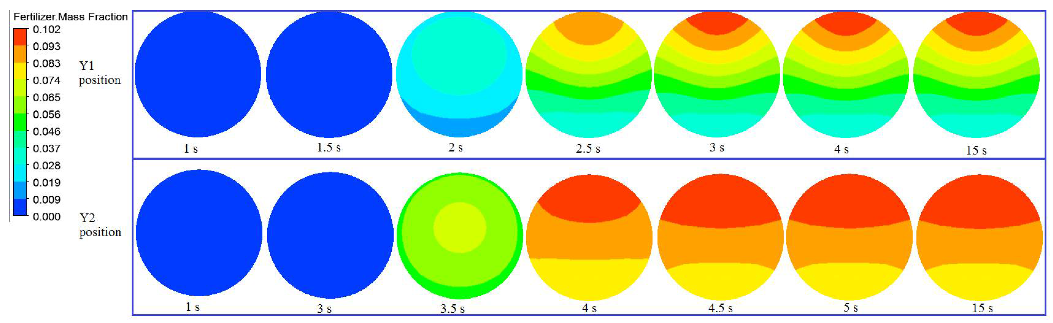
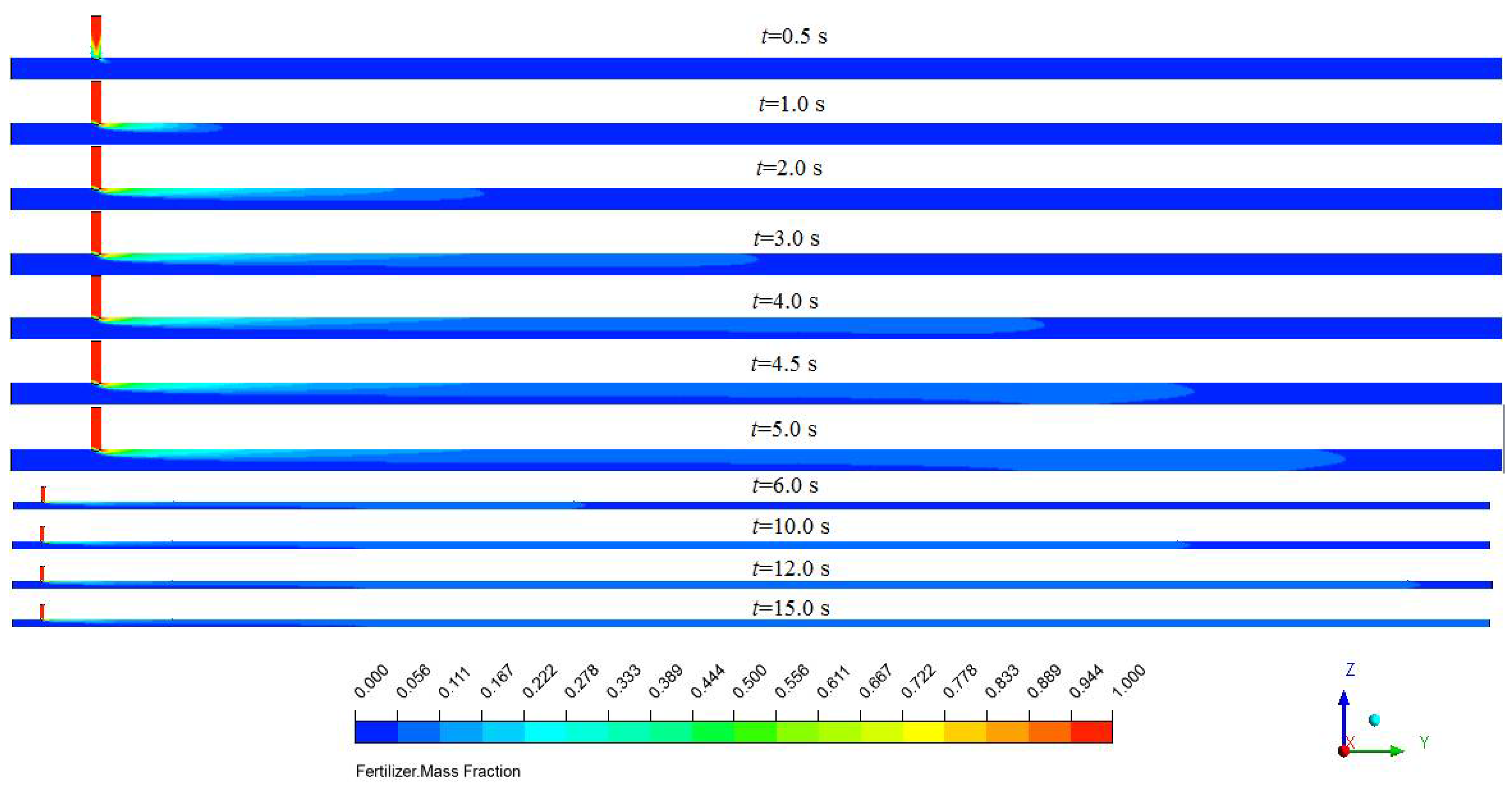
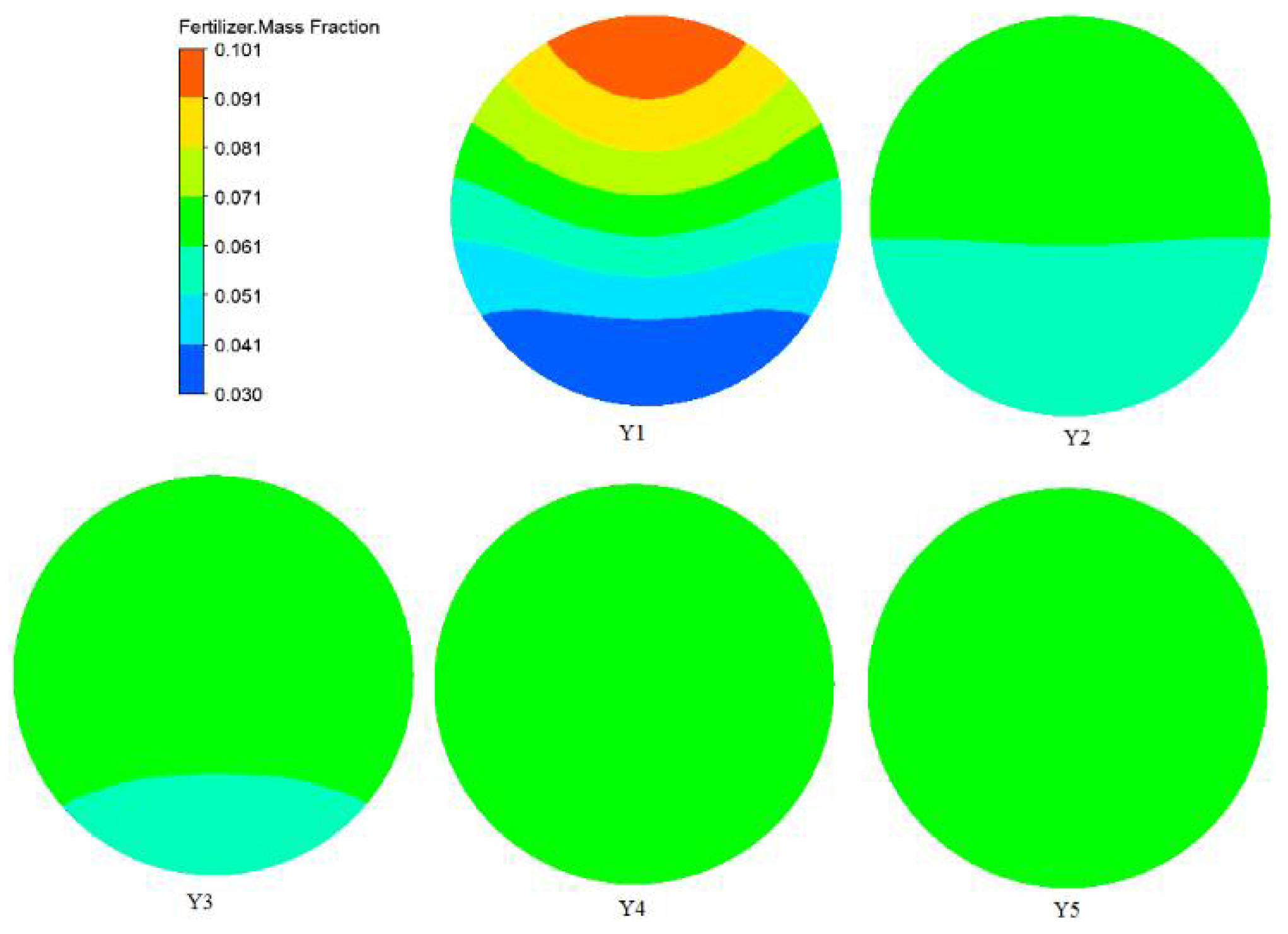
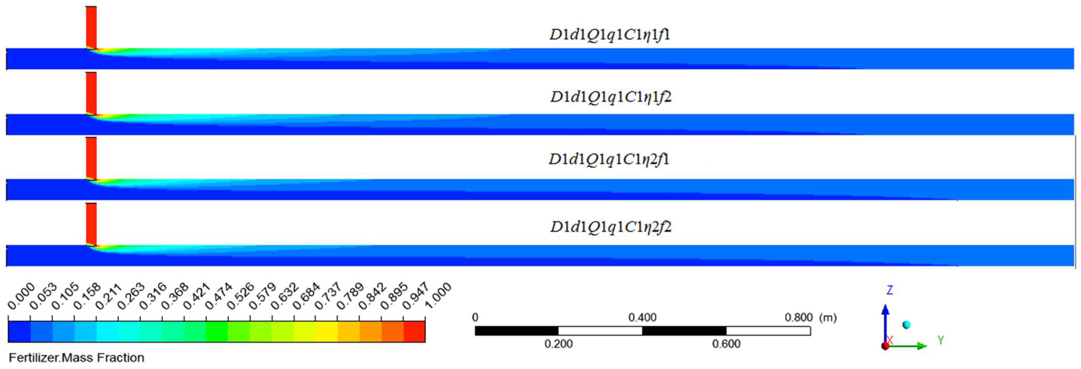
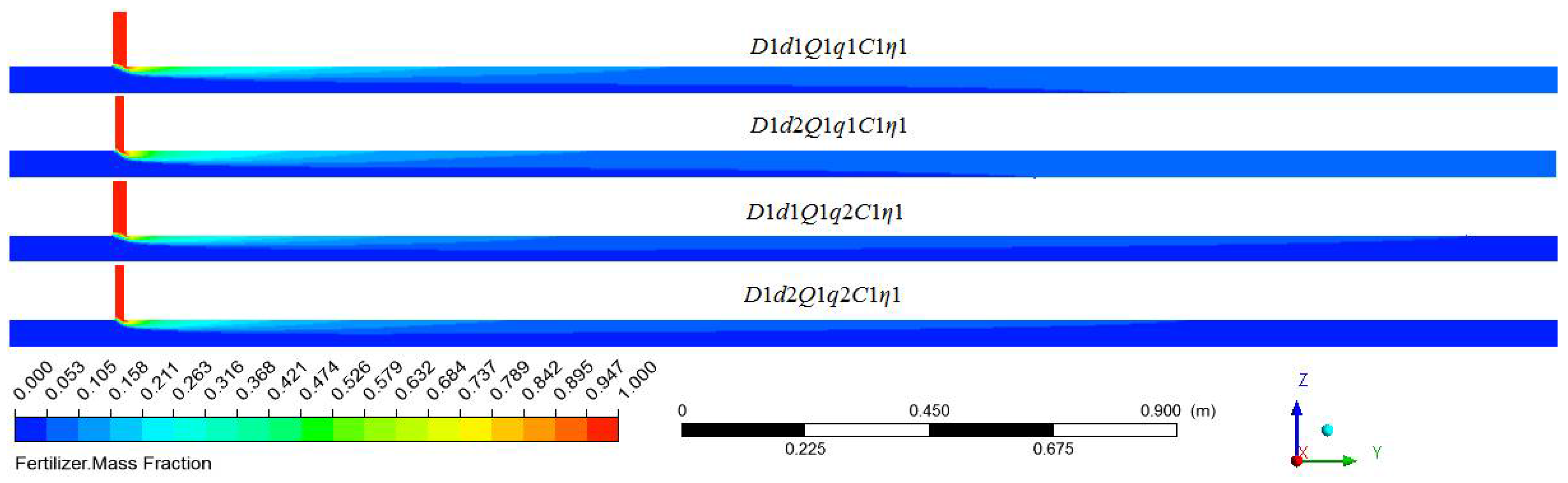
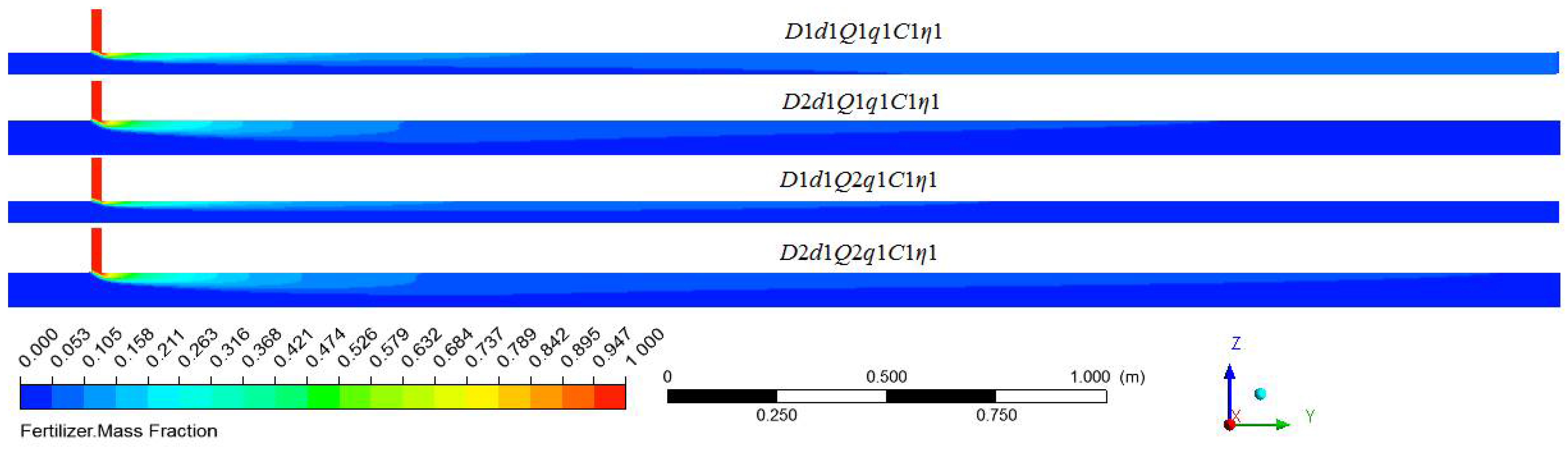
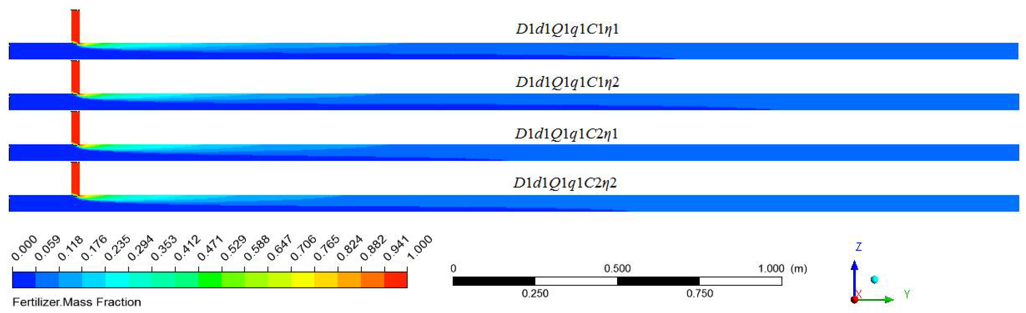
3.1. Fertilizer–Water Mixing State in the Pipes at Different Positions and Time

The first conducted simulation (condition of D1d1Q1q1C1η1f1) was chosen as an example to investigate the fertilizer–water mixing state in the pipes at different positions and time. The result is shown in Figure 7, where it was found that the fertilizer did not move to the Y1 position when it was injected for 1.5 s. The fertilizer mass fraction was 0.009–0.037 on the radial section at 2 s, indicating that a small amount of fertilizer had moved to the Y1 position as the water flowed. During 2 s and 2.5 s, more fertilizer moved to the Y1 position, and it presented a gradient distribution on the radial section. This results were kept consistent with a finding proposed by Widiatmojo et al. [22], who investigated the diffusion of a solute in turbulent flows through a circular pipe. Duda et al. [23] also reported that the concentration showed a gradient distribution when the polymer diffused in the solvent. The fertilizer mass fraction at the top of the section increased slightly when the time changed from 2.5 s to 3 s. After 3 s, the fertilizer mass fraction remained unchanged in the whole radial section. Similarly, on the radial section at the Y2 section, no fertilizer passed through the Y2 position during the first 3 s. Subsequently, the fraction of fertilizer mass increased, distributed in the gradient, and did not change after 4.5 s. After the flow in the pipe was stable, the fertilizer mass fraction at any position did not change with time in the areas where the fertilizer had flowed.
Figure 8 shows the distribution of the fertilizer mass fraction along the axis direction at different times after it had been injected into the pipeline. As shown, the fertilizer entered the water pipe after it was injected for 0.5 s. At any time, the fertilizer mass fraction of the area near the fertilizer pipe was high. It then decreased at the axial direction and the radial direction because as time progressed, the fertilizer would flow with water to the outlet and move in the radial direction. A comparison of the results at 4.0, 4.5, and 5.0 s indicated that the fertilizer mass fraction did not reach the same level along the radial direction at 4.0 s, but did at 4.5 s. Compared with 4.5 s, the fertilizer just continued to move toward the outlet at 5.0 s, and the change in the radial direction was almost invisible, as were the simulation results after 5.0 s. Moreover, the fertilizer had moved to the position that was closest to the outlet at 12.0 s and had filled the whole pipe system at 15.0 s.
The fertilizer mass fraction at any position did not change with time in areas where the fertilizer had flowed, and the fertilizer moved to the outlet in 15 s. Therefore, the simulation results at 15 s were selected as examples to investigate the distribution of fertilizer in the radial direction, obtain the COV variation, and confirm the uniform mixing length, the results of which are shown in Figure 9 and Figure 10. The fertilizer mass fraction on the radial section was symmetrical along the radial direction. In the upper half of the pipe, the fertilizer mass fraction deceased with the extension of the mixing length, while increased in the lower half. After Y4, the fertilizer mass fraction on the radial section was basically the same, indicating that the fertilizer had uniformly mixed with water between 3 and 4 m. Finally, the fertilizer mass fraction can be calculated using the following equation:
ω = ρ f q t ρ f q t + ρ w Q t = ρ f q ρ f q + ρ w Q
where ρf (kgm−3) is the density of the fertilizer. Substituting the parameters of the D1d1Q1q1C1η1f1 condition into Equation (14) resulted in a fertilizer mass fraction of 0.619, which was the same as that shown in Figure 9. The COV values of some of the axis positions were calculated using Equation (1), and the results are shown in Figure 10. It was obvious that the COV value decreased sharply at first and then slowly as the mixing length increased. The uniform mixing length of the D1d1Q1q1C1η1f1 condition was 3.64 m.

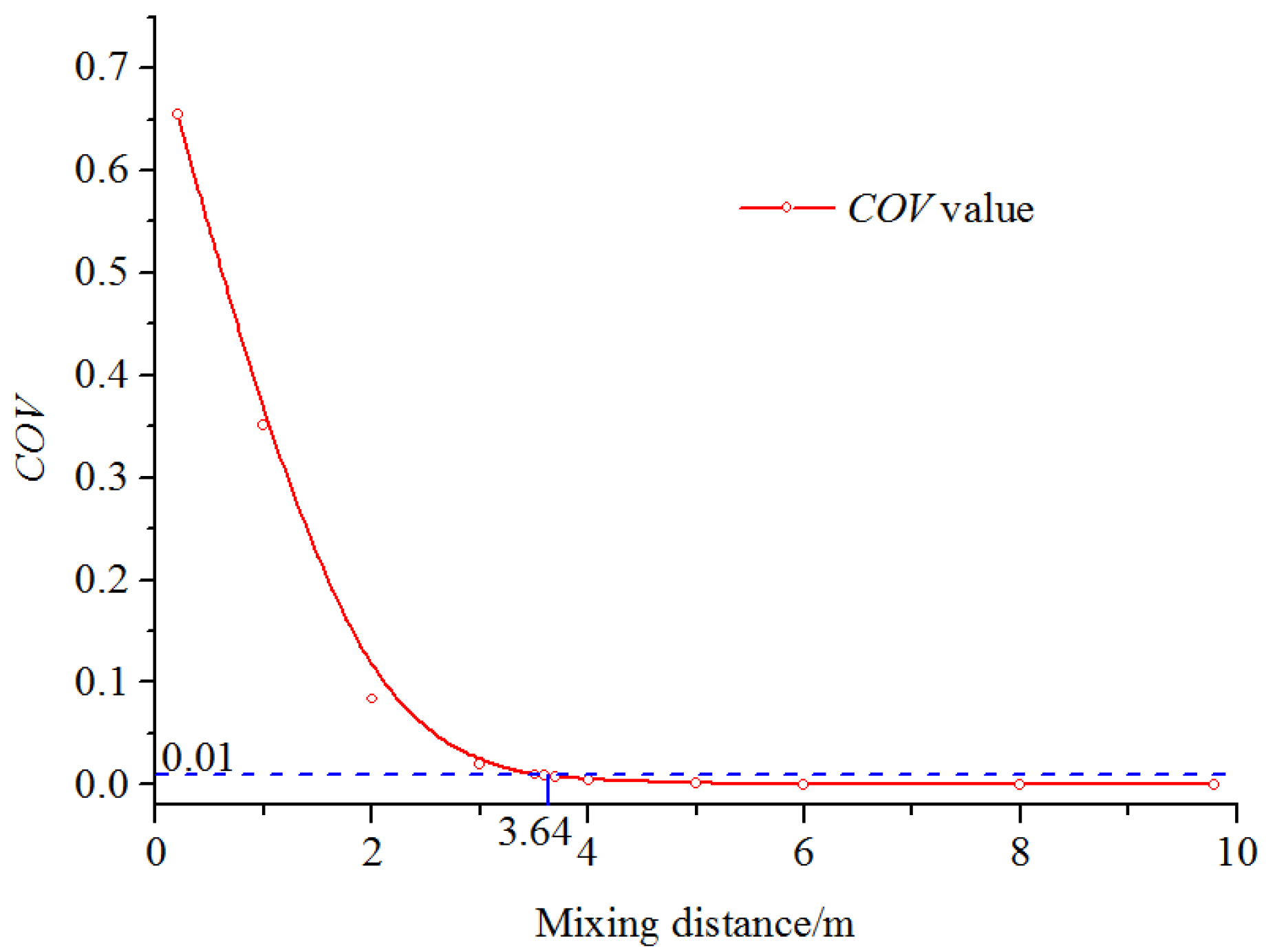
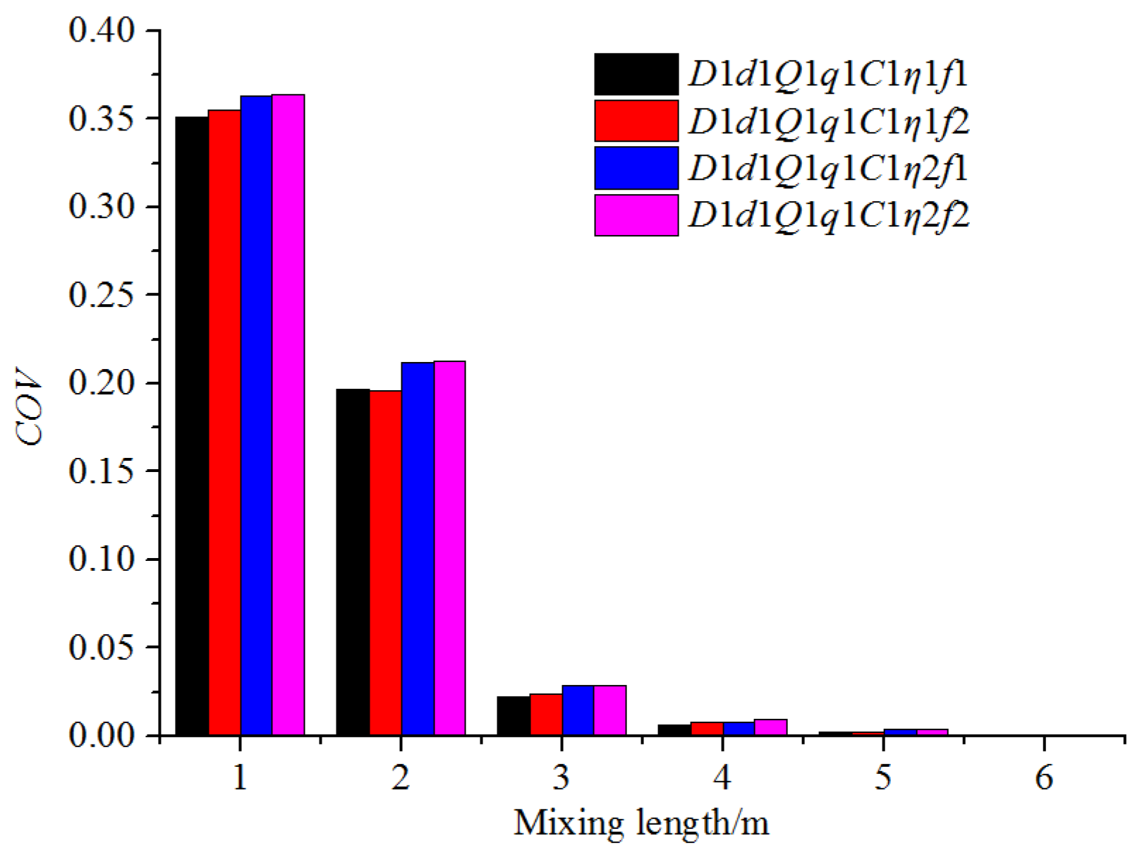
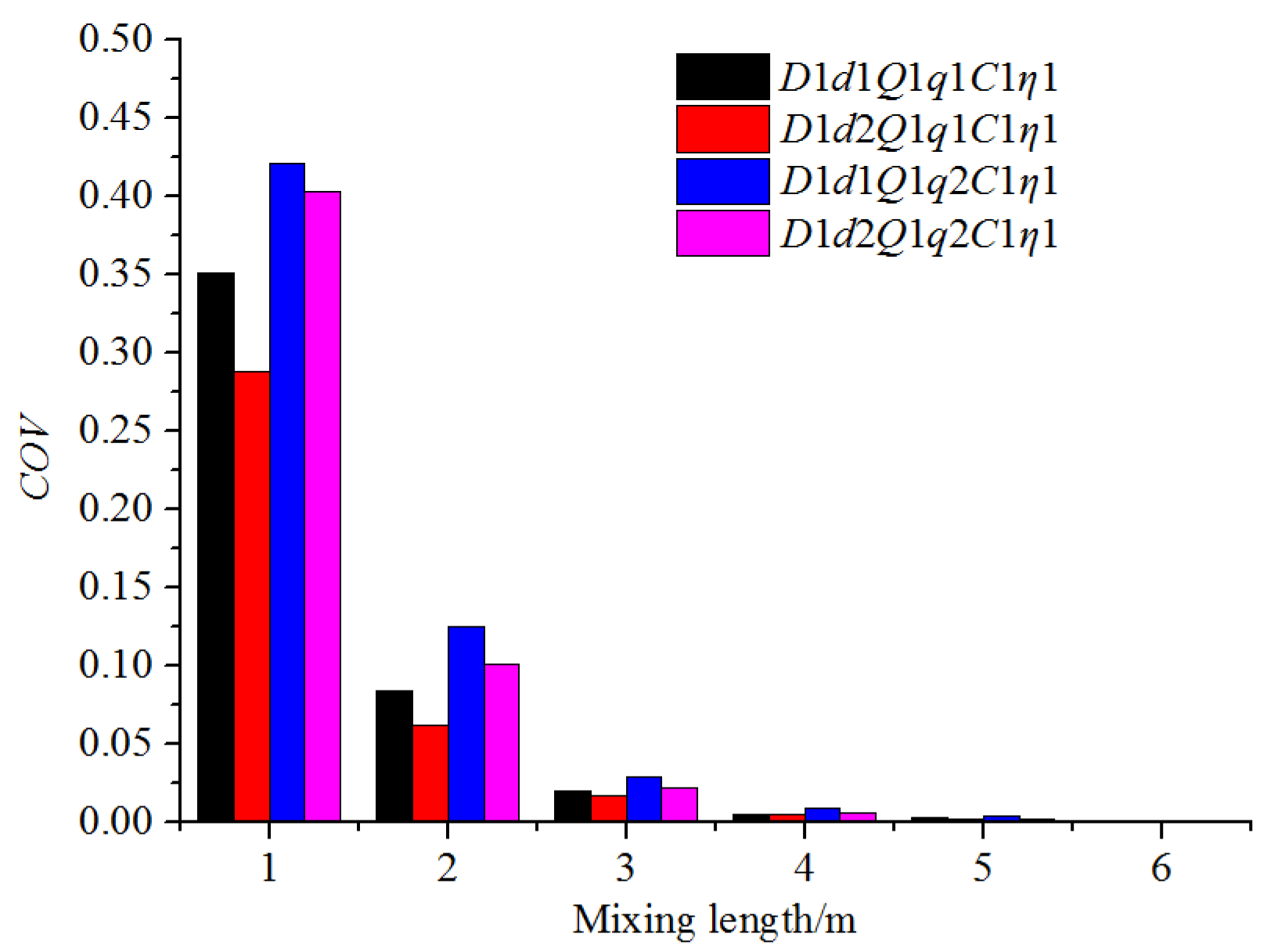
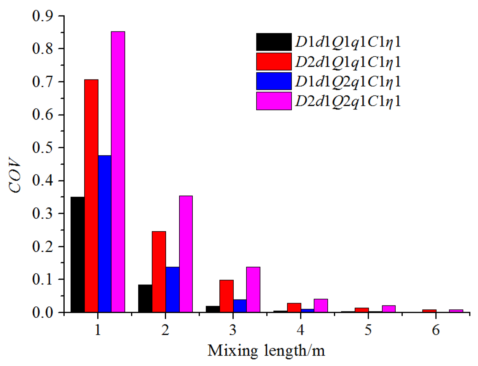
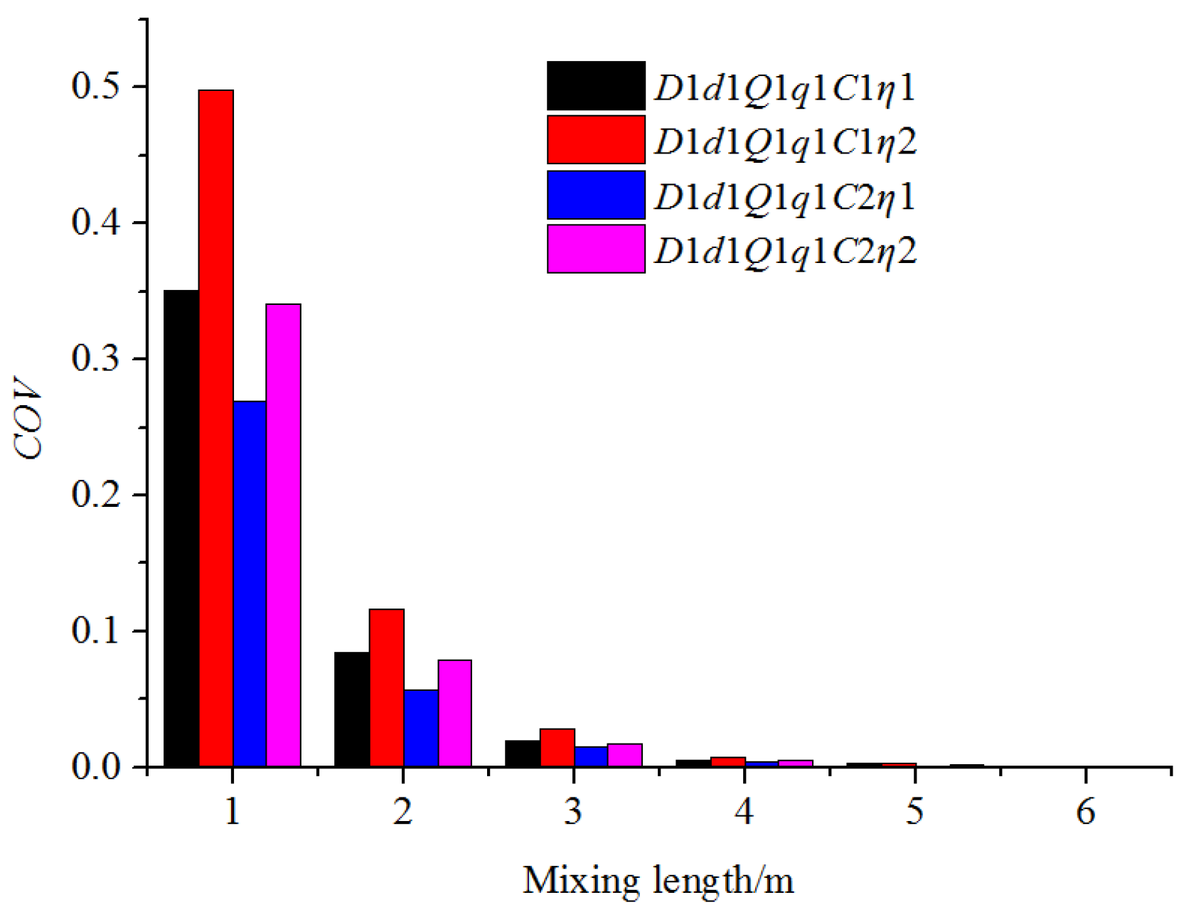
3.2. Factors Affecting the Mixing Speed and Uniform Mixing Length

Figure 11 shows the distribution of the fertilizer mass fraction along the water pipe under different fertilizer injection frequencies. The trend of fertilizer distribution was similar in four conditions. The fertilizer mass fraction in the upper section of the pipe was higher than that in the lower. The deviation of the fertilizer mass fraction in the pipe narrowed with the increase in the mixing distance. After a certain mixing distance in the simulated picture, the fertilizer mass fraction along the Z direction was at the same level. This distance can be used to roughly estimate the uniform mixing length in future research. When the only change was the frequency of the injection of fertilizer, the fertilizer distribution in pipe was the same, and the COV value at the same mixing distance was basically consistent, which was shown in Figure 12. The fertilizer injection frequency did not affect the fertilizer–water mixing law in the pipes, and, of course, would not affect the uniform mixing length. Therefore, the following research was able to neglect the factor of fertilizer injection frequency to reduce the unnecessary workload, and all the working conditions were in the f1 frequency.
The distribution of fertilizer mass fraction along the water pipe under different fertilizer pipe diameters and fertilizer flow rates is shown in Figure 13. The fertilizer was found to mix with water faster at the radial direction with the increase in the fertilizer flow rate and the decrease in the diameter of the fertilizer pipe. This was because a larger flow rate and a smaller fertilizer pipe diameter resulted in an increase in the speed of fertilizer that was injected into the pipe, enabling the fertilizer to move a longer distance along the radial direction within the same amount of time. In these four conditions, the mixing distance that enabled the fertilizer mass fraction to be at the same level differed significantly. Smaller fertilizer flow rates and a larger diameter of the fertilizer pipe resulted in a longer uniform mixing length. Figure 14 shows the COV variation along the mixing distance under different fertilizer pipe diameters and fertilizer flow rates. The COV value at the same axis position decreased with the increase in the fertilizer flow rates and a reduction in the diameter of the fertilizer pipe, which also indicated that the uniform mixing length would be long when the fertilizer pipe was large, and the fertilizer flow rates were small. With the increase in the mixing length, the COV gap of four conditions narrowed. For example, when the mixing length was 1 m, the COV value of D1d2Q1q1C1η1 was 0.063 less than that of D1d1Q1q1C1η1, but 0.022 less when the mixing length exceeded 2 m. The uniform mixing length was between 3 and 4 m in all four working conditions.
The fertilizer distribution along the water pipe under different flow rates of water and water pipe diameters are shown in Figure 15, which compares the simulation results of D1d1Q1q1C1η1, D2d1Q1q1C1η1, D1d1Q2q1C1η1, and D2d1Q2q1C1η1. It was apparent that as the water pipe diameter increased and the water flow rate decreased, the fertilizer moved a longer distance along the Z direction at the same axis position, and so the mixing speed at the radial direction was faster. The mixing length that resulted in the fertilizer mass fraction being at the same level was more backward when the water flow rate and the water pipe diameter were larger. Figure 16 indicates the COV variation along the axis of the water pipe under four working conditions. When examined at the same axis position, larger flow rates and larger water pipe diameters resulted in a higher COV value. The uniform mixing length under the four working conditions, from long to short, were D2Q2, D2Q1, D1Q2, and D1Q1. Thus, the uniform mixing length was proportional to the water pipe diameter and flow rates of water.
The effect of the fertilizer concentration and viscosity on the mixing law is shown in Figure 17. It is apparent that there was no obvious difference in the distribution of fertilizer in the Z direction under four conditions. The fertilizer distribution in the Y direction indicated that as the concentration of fertilizer became higher and the viscosity smaller, the uniform mixing length would be longer. Because diffusion is essentially the transfer of matter molecules from a high region of concentration to one of low concentration, the diffusion rate is proportional to the concentration difference. These results were consistence with a finding proposed by Olaye et al. [24], who developed a numerical diffusion model to study the dependence of the interdiffusion coefficient on concentration. Amsden et al. [25] also found the relationship between concentration and diffusion rate by the proposed solute diffusion prediction model. Moreover, according to Stokes Einstein Theory [26], the diffusion coefficient of the solutes in solvent is inversely proportional to the viscosity of the solute. Thus, a higher diffusion coefficient results in faster diffusion rates. Figure 18 shows the variation in the COV value along the axis of the water pipe in four conditions. At the same axis position, the COV value decreased with an increase in the concentration of the fertilizer and a decrease in the viscosity. The uniform mixing lengths in all four cases were between 3 and 4 m, and the longest uniform mixing length was under C1η2 conditions, thus following the C1η1, C2η2, and C2η1 condition.

3.3. Dimensional Analysis of the Uniformity Mixing Length

To predict the uniform mixing length under different pipeline structure parameters, hydraulic parameters, and fertilizer physical properties, the relationship between them was established through dimensional analysis. Dimensional analysis is a method to analyze and judge the general law of the quantitative relationship between things based on the necessary form of all quantities [27]. It can be used to solve the criterion relationship when problems cannot be described by a differential equation. To explore the relationship between each factor, it is necessary to determine the main physical quantities that affect the physical process [28]. Based on the analysis of factors that influence the uniform mixing length, seven physical quantities including the uniform mixing length (Lu), water pipe diameter (D), water flow rate (Q), viscosity of fertilizer solution (η), fertilizer pipe diameter (d), fertilizer flow rate (q), and fertilizer concentration (C) were chosen to obtain the dimensional relationship.
f ( D , η , Q , d , q , C , L u ) = 0
According to the π theorem, three independent quantities (D, Q, μ) were adopted as the basic quantities, so that Equation (15) is dimensionless:
f ( 1 , 1 , 1 , π 1 , π 2 , π 3 , π 4 ) = 0
{ π 1 = d D π 2 = q Q π 3 = C η D Q 1 π 4 = L u D
Equation (18) can be obtained:
π 4 = L u D = f ( 1 , 1 , 1 , d D , q Q , C Q η D )
Then, Equation (18) can be transformed into Equation (19) as follows:
L u D = a ( d D ) b ( q Q ) e ( C Q η D ) f
The uniform mixing lengths under different working conditions are shown in Table 4. The fitting coefficient a, b, e, and f can be obtained by substituting the data in Table 4 into Equation (19), and Lu can be estimated through Equation (20):
L u = 76.614 D 0.903 d 0.144 Q 0.22 q - 0.267 ( C η ) - 0.047 ( R 2   = 0.936 )
The correlation coefficient (R2) was 0.936, which greatly exceeded 0.8, indicating that there was a strong correlation between the uniform mixing length and six variables in Equation (20). When all 64 simulation conditions were substituted into Equation (20), the uniform mixing length calculated by Equation (20) was found to be close to the simulation results. The maximum, minimum, and average relative errors were 4.64%, 0.01%, and 1.95%, respectively. Thus, Equation (20) can accurately predict the uniform mixing length.

4. Conclusions

(1) A CFD simulation method based on the species transport model was proposed to study the mixing law of fertilizer and water in the irrigation pipe. The average deviation of the experimental and simulation results was 5.71%. In areas where the fertilizer had flowed, the fertilizer mass fraction at any position in the pipe did not change with time.
(2) The fertilizer injection frequency did not affect the fertilizer–water mixing law in the pipe. With the increase in the fertilizer flow rate (q) and water pipe diameter (D) and the decrease in the fertilizer pipe diameter (d) and water flow rate (Q), the speed at which the fertilizer mixed with water along the radial direction increased significantly. The uniform mixing length (Lu) was directly proportional to the fertilizer pipe diameter, water pipe diameter, water flow rate, and fertilizer viscosity(η) was inversely proportional to the fertilizer flow rate and fertilizer concentration (C).
(3) The relationship between the mixing uniform length and six variables (water pipe diameter, fertilizer pipe diameter, water flow rate, fertilizer flow rate, fertilizer concentration and viscosity) was fitted by a dimensional analysis. The R2 of the fitting equation was 0.936, and the equation can be used to predict the uniform mixing length under other working conditions.

Author Contributions

Z.Z. and P.T. conceived and structured the simulation methods and the testing system. Z.Z. and C.C. performed the literature search, helped in the experiments, and analyzed the test data. Z.Z. and H.L. wrote the paper and approved the submitted version of the manuscript. All authors have read and agreed to the published version of the manuscript.

Funding

This work was supported by National Natural Science Foundation of China (grant number 51939005); Key Research and Developement Program of Jiangsu Province (grant number BE2021340, BE2021379); Demonstration and Promotion Project of Modern Agricultural Machinery Equipment and Technology of Jiangsu Province (SJC20210194); and A Project Funded by the Priority Academic Program Development of Jiangsu Higher Education Institutions (grant number PAPD-2018-87).

Acknowledgments

The authors are thankful to the editor and reviewers for their valuable comments in improving the quality of this paper.

Conflicts of Interest

The authors declare no conflict of interest.

References

  1. Zhang, X.; Bol, R.; Rahn, C.; Xiao, G.; Meng, F.; Wu, W. Agricultural sustainable intensification improved nitrogen use efficiency and maintained high crop yield during 1980–2014 in Northern China. Sci. Total Environ. 2017, 596–597, 61–68. [Google Scholar] [CrossRef]
  2. Kaplan, M.; Kara, K.; Unlukara, A.; Kale, H.; Beyzi, S.B.; Varol, I.S.; Kizilsimsek, M.; Kamalak, A. Water deficit and nitrogen affects yield and feed value of sorghum sudangrass silage. Agric. Water Manage. 2019, 218, 30–36. [Google Scholar] [CrossRef]
  3. Stefani, I.E.A.; Roberto, K.H.G.; Mario, C.U.A.; Sillas, H. Video-based fractional order identification of diffusion dynamics for the analysis of migration rates of polar and nonpolar liquids: Water and oil studies. Rev. Sci. Instrum. 2021, 92, 035106. [Google Scholar]
  4. Han, H.; Furst, E.M.; Kim, C. Lagrangian analysis of consecutive images: Quantification of mixing processes in drops moving in a microchannel. Rheol. Acta 2014, 53, 489–499. [Google Scholar] [CrossRef]
  5. Hansen, L.; Guilkey, J.E.; Mcmurtry, P.A.; Klewicki, J.C. The use of photoactivatable fluorophores in the study of turbulent pipe mixing: Effects of inlet geometry. Meas. Sci. Technol. 2000, 11, 1235. [Google Scholar] [CrossRef]
  6. Ger, A.M.; Holley, E.R. Comparison of single-point injections in pipe flow. J. Hydraul. Div. 1976, 102, 731–746. [Google Scholar] [CrossRef]
  7. Nakayama, H.; Hirota, M.; Shinoda, K.; Koide, S. Flow and mixing characteristics in counter-type t-junction (influence of flow ratio on mixing characteristics). Trans. Jpn. Soc. Mech. Eng. Part B 2007, 73, 1813–1820. [Google Scholar] [CrossRef]
  8. Mi, Z.; Kulenovic, R.; Laurien, E. T-junction experiments to investigate thermal-mixing pipe flow with combined measurement techniques. Appl. Therm. Eng. 2018, 150, 237–249. [Google Scholar]
  9. Enrique, L.; Aguila, E. Application of sprinkler system for nitrogen fertilization in corn. Rev. Fac. Agron. 2019, 36, 490–496. [Google Scholar]
  10. Finzi, A.; Guido, V.; Riva, E.; Ferrari, O.; Provolo, G. Performance and sizing of filtration equipment to replace mineral fertilizer with digestate in drip and sprinkler fertigation. J. Clean. Prod. 2021, 317, 128431. [Google Scholar] [CrossRef]
  11. Zughbi, H.D. Effects of jet protrusion on mixing in pipelines with side-tees. Chem. Eng. Res. Des. 2006, 84, 993–1000. [Google Scholar] [CrossRef]
  12. Lateef, M.O.; Olusola, K.; John, A. On the numerical simulation of turbulent pipe flow pattern using comsol multiphysics. Int. J. Sci. World 2013, 1, 13–18. [Google Scholar]
  13. Lin, G.H.; Chen, M.S.; Ferng, Y.M. Investigating thermal mixing and reverse flow characteristics in a t-junction using cfd methodology. Appl. Therm. Eng. 2016, 102, 733–741. [Google Scholar] [CrossRef]
  14. Sun, B.; Lu, Y.; Liu, Q.; Fang, H.; Zhang, C.; Zhang, J. Experimental and numerical analyses on mixing uniformity of water and saline in pipe flow. Water 2020, 12, 2281. [Google Scholar] [CrossRef]
  15. Tang, P.; Li, H.; Issaka, Z.; Chen, C. Effect of manifold layout and fertilizer solution concentration on fertilization and flushing times and uniformity of drip irrigation systems. Agri. Water Manag. 2018, 200, 71–79. [Google Scholar] [CrossRef]
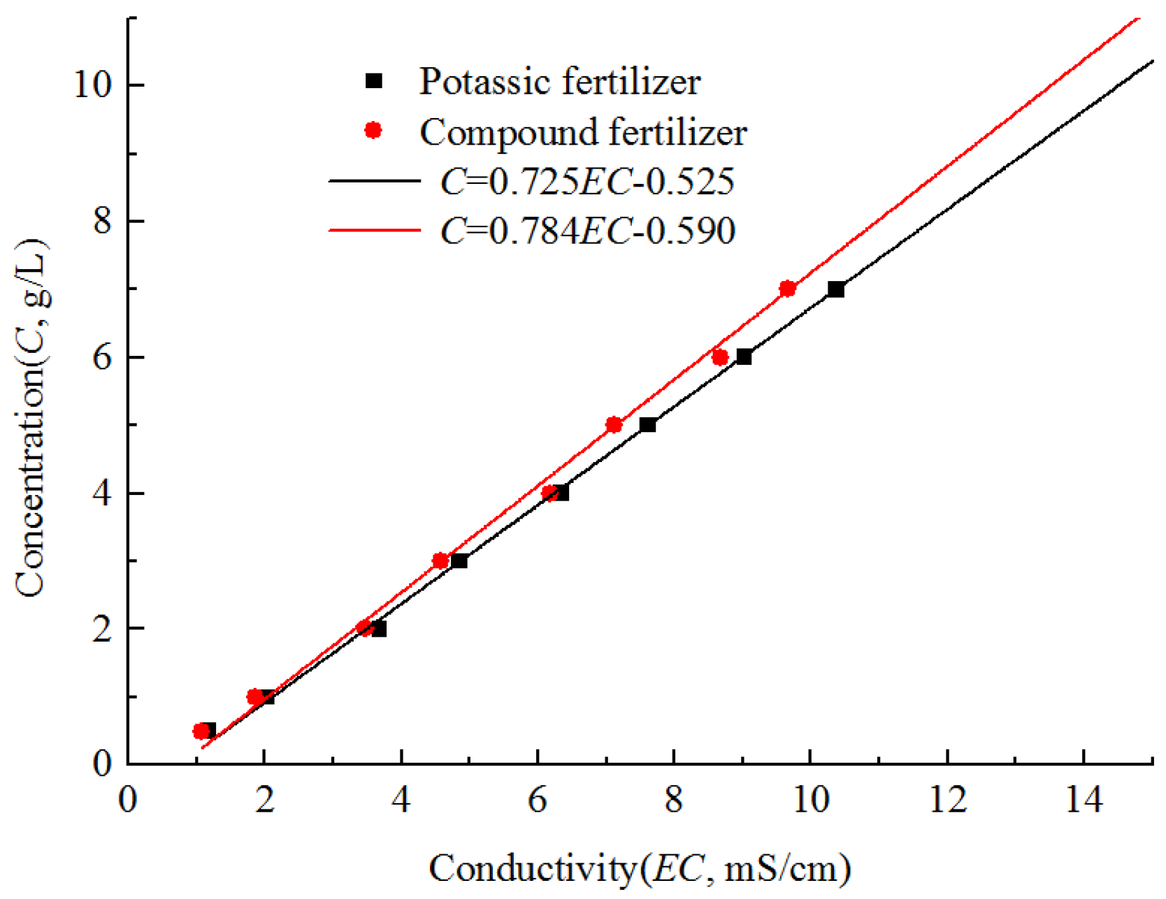
  16. Saoudi, O.; Ghaouar, N.; Othman, T. Conductivity measurements of laccase for various concentrations, pH and ionic liquid solutions. Fluid Phase Equilib. 2017, 443, 184–192. [Google Scholar] [CrossRef]
  17. Somkhuean, R.; Niwitpong, S.; Niwitpong, S.A. Upper Bounds of Generalized p-values for Testing the Coefficients of Variation of Lognormal Distributions. Chiang Mai J. Sci. 2016, 43, 672–682. [Google Scholar]
  18. Mohammed, H.I.; Giddings, D.; Walker, G.S. CFD simulation of a concentrated salt nanofluid flow boiling in a rectangular tube. Int. J. Heat Mass Transf. 2018, 125, 218–228. [Google Scholar] [CrossRef]
  19. Tang, P.; Juárez, J.M.; Li, H. Investigation on the effect of structural parameters on cavitation characteristics for the venturi tube using the cfd method. Water 2019, 11, 2194. [Google Scholar] [CrossRef] [Green Version]
  20. Spiessl, S.M.; Prommer, H.; Licha, T.; Sauter, M.; Zheng, C. A process-based reactive hybrid transport model for coupled discrete conduit–continuum systems. J. Hydrol. 2007, 347, 23–34. [Google Scholar] [CrossRef]
  21. Sugiharto; Stegowski, Z.; Furman, L.; Su’Ud, Z.; Abidin, Z. Dispersion determination in a turbulent pipe flow using radiotracer data and cfd analysis. Comput. Fluids. 2013, 79, 77–81. [Google Scholar] [CrossRef]
  22. Widiatmojo, A.; Sasaki, K.; Widodo, N.P.; Sugai, Y. Discrete tracer point method to evaluate turbulent diffusion in circular pipe flow. J. Flow Control. Meas. Vis. 2013, 1, 57–68. [Google Scholar] [CrossRef] [Green Version]
  23. Duda, J.L.; Vrentas, J.S.; Ju, S.T.; Liu, H.T. Prediction of diffusion coefficients for polymer-solvent systems. AIChE J. 2010, 28, 279–285. [Google Scholar] [CrossRef]
  24. Olaye, O.; Ojo, O. Time variation of concentration-dependent interdiffusion coefficient obtained by numerical simulation analysis. Materialia 2021, 16, 101056. [Google Scholar] [CrossRef]
  25. Amsden, B. Solute diffusion within hydrogels. mechanisms and models. Macromolecules 1998, 31, 8382–8395. [Google Scholar] [CrossRef]
  26. Mazza, M.G.; Giovambattista, N.; Stanley, H.E.; Starr, F.W. Connection of translational and rotational dynamical heterogeneities with the breakdown of the stokes-einstein and stokes-einstein-debye relations in water. Phys. Rev. E 2007, 76, 031203. [Google Scholar] [CrossRef] [PubMed] [Green Version]
  27. Asce, K.S.L.M.; Reeuwijk, M.V.; Maksimovic, C. Simplified numerical and analytical approach for solutes in turbulent flow reacting with smooth pipe walls. J. Hydraul. Eng. 2010, 136, 626–632. [Google Scholar]
  28. Lari, K.S.; van Reeuwijk, M.; Maksimovic, C.; Sharifan, S. Combined bulk and wall reactions in turbulent pipe flow: Decay coefficients and concentration profiles. J. Hydroinform. 2011, 13, 324–333. [Google Scholar] [CrossRef] [Green Version]
Figure 1. Experimental equipment site. (1) Water tank, (2) Centrifugal pump, (3) Fertilizer injection pipe, (4) Flowmeter, (5) Sampling point, (6) PE transparent pipe, (7) Plunger pump, and (8) Fertilizer tank.
Horticulturae 08 00200 g001
Figure 2. Sampling point arrangement (unit: mm).
Horticulturae 08 00200 g002
Figure 3. Relationship between the concentration and conductivity of two fertilizers.
Horticulturae 08 00200 g003
Figure 4. Geometric model of the mixing pipe system.
Horticulturae 08 00200 g004
Figure 5. Numerical models of the inner flow channel of the mixing pipeline.
Horticulturae 08 00200 g005
Figure 6. Comparison of experimental and simulated results of four selected cases. (a) Fertilizer mass fraction at the upper section of the pipe. (b) Fertilizer mass fraction at the lower section of the pipe.
Horticulturae 08 00200 g006
Figure 7. Variation of fertilizer mass fraction with time on the radial section at the Y1 and Y2 positions.
Horticulturae 08 00200 g007
Figure 8. Distribution of fertilizer mass fraction along the axis direction at different times.
Horticulturae 08 00200 g008
Figure 9. Distribution of fertilizer mass fraction along the radial direction at different axis positions.
Horticulturae 08 00200 g009
Figure 10. COV value variation along the axis of the water pipe (D1d1Q1q1C1η1f1).
Horticulturae 08 00200 g010
Figure 11. Distribution of fertilizer mass fraction along the water pipe under different fertilizer injection frequencies.
Horticulturae 08 00200 g011
Figure 12. COV variation along the mixing distance under different fertilizer injection frequencies.
Horticulturae 08 00200 g012
Figure 13. Distribution of fertilizer mass fraction along the water pipe under different fertilizer pipe diameters and fertilizer flow rates.
Horticulturae 08 00200 g013
Figure 14. COV variation along the mixing distance under different fertilizer flow rates and fertilizer pipe diameters.
Horticulturae 08 00200 g014
Figure 15. Distribution of fertilizer mass fraction along the water pipe under different flow rates of water and water pipe diameters.
Horticulturae 08 00200 g015
Figure 16. COV variation along the mixing distance under different flow rates of water and water pipe diameters.
Horticulturae 08 00200 g016
Figure 17. Distribution of fertilizer mass fraction along the mixing distance under different fertilizer concentrations and viscosities.
Horticulturae 08 00200 g017
Figure 18. COV variation along the axis of the water pipe under different fertilizer concentrations.
Horticulturae 08 00200 g018
Table 1. Relationship between the viscosity and concentration of the potassium chloride and compound fertilizer.
Concentration (gL−1)125102050100200
Viscosity (kgm−1s−1)Compound fertilizer0.00210.00220.00220.00220.00230.00220.00220.0022
Potassium chloride0.00550.00550.00550.00550.00540.00530.00550.0055
Table 2. Experimental design to investigate the fertilizer–water mixing law in the irrigation pipe.
LevelsFactors
D (m)d (m)Q (m3h−1)q (m3h−1)C (gL−1)η (kgm−1s−1)f (HZ)
10.050.02550.31000.00222
20.080.01580.22000.00554
Table 3. Mesh independence study for D1d1Q1q1C1η1f1 conditions.
Number of CellsFertilizer Mass Fraction
Upper of Y1Lower of Y1Upper of Y2Lower of Y2Upper of Y3Lower of Y3
2,432,0070.1010.3050.6990.5410.6390.599
2,625,4800.1000.3020.7020.5390.6310.606
2,932,5800.1000.3190.7090.5230.6250.607
Table 4. Uniform mixing length (m) under different working conditions.
GroupLuGroupLuGroupLuGroupLu
D1d1Q1q1C1η13.64D1d2Q1q1C1η13.46D2d1Q1q1C1η15.55D2d2Q1q1C1η15.15
D1d1Q1q1C1η23.75D1d2Q1q1C1η23.51D2d1Q1q1C1η25.71D2d2Q1q1C1η25.38
D1d1Q1q1C2η13.32D1d2Q1q1C2η13.18D2d1Q1q1C2η15.31D2d2Q1q1C2η14.94
D1d1Q1q1C2η23.55D1d2Q1q1C2η23.33D2d1Q1q1C2η25.42D2d2Q1q1C2η25.29
D1d1Q1q2C1η13.88D1d2Q1q2C1η13.59D2d1Q1q2C1η16.05D2d2Q1q2C1η15.56
D1d1Q1q2C1η24.05D1d2Q1q2C1η23.89D2d1Q1q2C1η26.13D2d2Q1q2C1η26.01
D1d1Q1q2C2η13.73D1d2Q1q2C2η13.48D2d1Q1q2C2η15.75D2d2Q1q2C2η15.43
D1d1Q1q2C2η23.93D1d2Q1q2C2η23.63D2d1Q1q2C2η25.98D2d2Q1q2C2η25.79
D1d1Q2q1C1η14.08D1d2Q2q1C1η13.83D2d1Q2q1C1η15.93D2d2Q2q1C1η15.74
D1d1Q2q1C1η24.34D1d2Q2q1C1η23.95D2d1Q2q1C1η26.21D2d2Q2q1C1η26.05
D1d1Q2q1C2η13.92D1d2Q2q1C2η13.63D2d1Q2q1C2η15.83D2d2Q2q1C2η15.32
D1d1Q2q1C2η24.15D1d2Q2q1C2η23.81D2d1Q2q1C2η26.11D2d2Q2q1C2η25.76
D1d1Q2q2C1η14.51D1d2Q2q2C1η14.26D2d1Q2q2C1η16.52D2d2Q2q2C1η16.22
D1d1Q2q2C1η24.71D1d2Q2q2C1η24.43D2d1Q2q2C1η26.96D2d2Q2q2C1η26.55
D1d1Q2q2C2η14.32D1d2Q2q2C2η13.92D2d1Q2q2C2η16.39D2d2Q2q2C2η16.03
D1d1Q2q2C2η24.47D1d2Q2q2C2η24.11D2d1Q2q2C2η26.68D2d2Q2q2C2η26.32
Publisher’s Note: MDPI stays neutral with regard to jurisdictional claims in published maps and institutional affiliations.

