Automation for Water and Nitrogen Deficit Stress Detection in Soilless Tomato Crops Based on Spectral Indices

Abstract

Water and nitrogen deficit stress are some of the most important growth limiting factors in crop production. Several methods have been used to quantify the impact of water and nitrogen deficit stress on plant physiology. However, by performing machine learning with hyperspectral sensor data, crop physiology management systems are integrated into real artificial intelligence systems, providing richer recommendations and insights into implementing appropriate irrigation and environment control management strategies. In this study, the Classification Tree model was used to group complex hyperspectral datasets in order to provide remote visual results about plant water and nitrogen deficit stress. Soilless tomato crops are grown under varying water and nitrogen regimes. The model that we developed was trained using 75% of the total sample dataset, while the rest (25%) of the data were used to validate the model. The results showed that the combination of MSAVI, mrNDVI, and PRI had the potential to determine water and nitrogen deficit stress with 89.6% and 91.4% classification accuracy values for the training and testing samples, respectively. The results of the current study are promising for developing control strategies for sustainable greenhouse production.

1. Introduction

Nowadays, the need to produce more food with fewer inputs (water, fertilizer, and land, among others) and zero effect on the environment has led to an increase in greenhouse production. However, to cultivate under greenhouse conditions is certainly not an easy task since performance of several farming practices are needed. In this manner, crop yield and quality optimisation will be further improved only if farmers integrate greenhouse control strategies, that is, measurements concerning the dynamic response of plants according to the greenhouse’s spatial environment changes.

Within a greenhouse, however, it is a challenge to quantify the spatial impact of biotic or abiotic factors in plant growth. Usually, up to now, environmental patterns under greenhouses have been monitored and managed by sampling at a single position and by considering the indoor microclimate completely homogeneous [1]. This assumption, however, is not valid since an intense heterogeneity that must be taken into account actually occurs, especially in intensive production systems. A sensing system equipped with a multi-sensor platform moving over the canopy is the key to communicate the plant’s real state and needs. Obviously, in such moving platforms, the continuous monitoring of the interactions between the microclimate and the physical conditions of the plants is performed using mostly non-contact and non-destructive sensing techniques [2].

Up to now, the methods used for monitoring plant physiology have been quite complex and problematic. Most of these measure plant physiology in a limited spatial scale and, in most cases, they require physical contact with the plants/soil or follow destructive sensing procedures, making their application as a commercial multi-sensor scale rather infeasible [2,3,4].

The current development of computational hyperspectral machine vision systems allows us to build a real-time plant canopy health, growth, and quality monitoring multisensory platform equipped with remote technologies [5,6,7]. Hyperspectral machine vision systems allow recording in large scale, the spatial interaction of sunlight with crop canopies and plant leaves providing valuable information about plant growth and health status [6,8]. In this way, changes observed in plant irradiance of visible (VIS) and near infrared (NIR) spectrum, indicate different types of plant stress. The reflectance variation in VIS spectrum, for instance, is recorded to assess a series of several pigments located in the mesophyll area, such as chlorophyll, carotenoids and xanthophyll. The reflectance variation, on the other hand, observed in the NIR spectrum, is recorded to obtain information about leaf water content stored in cavities of spongy parenchyma. Additionally, changes in NIR spectrum are used to assess the carbon content in different forms (sugar, starch, cellulose and lignin) in mesophyll cells and nutrient compounds (N, P, K) in mesophyll cells and palisade parenchyma [2].

In order to provide more precise information for stress detection, certain parts of the spectrum can be combined to form reflectance indices (RIs) [2,7,9,10]. In this way, the spectral differences detected are amplified while the resulting RIs are used directly as a metric to quantify different aspects of plant physiology response.

So far, numerous successful case studies related to RIs and their relationship with crop, climate, or soil data from different plants have been performed. The photochemical reflectance index (PRI = (R₅₃₁ − R₅₇₀)/(R₅₃₁ + R₅₇₀)) is one of the most widespread indicators estimating rapid changes in de-epoxidation of the xanthophyll cycle [11,12,13,14]. Bajwa et al. [15] used the Modified soil-adjusted vegetation index (MSAVI = 1/2 × (2 × (R₈₁₀ + 1) − (√(2 × R₈₁₀ + 1) × 2 − 8 × (R₈₁₀ − R₆₉₀))) to predict green biomass (R² > 0.70). Elvanidi et al. [1,7,13] also showed that Modified red normalised vegetation and simple ration indices (mrNDVI = (R₇₅₀ − R₇₀₅)/(R₇₅₀ + R₇₀₅ − 2 × R₄₄₅); mrSRI = (R₇₅₀ − R₄₄₅)/(R₇₀₅ − R₄₄₅)) were the two most relevant and sensitive indices indicating water deficit stress in tomato plants. Additionally, the Transformed chlorophyll absorption in the reflectance index (TCARI = 3 × [(R₇₀₀ − R₆₇₀) − 0.2 × (R₇₀₀ − R₅₅₀) × (R₇₀₀/R₆₇₀)] was strongly correlated with leaf chlorophyll content variation [13,16].

In addition to reflectance indices, many statistical and machine learning models such as classification tree analysis, support vector machine, artificial neural network, and other classification procedures have been developed to extract optimal information from remotely sensed data [1]. Researchers observed that the classification tree (CT) was a very useful model to analyze complex data sets by providing visual results [13,17,18,19].

Therefore, the object of this work was to develop a model based on the CT method to analyse complex RIs datasets in order to provide visual assessments of plant water and nitrogen deficit stress. For this reason, RIs that indicate different aspects of tomato crop physiology (such as photosynthetic rate (As, μmol m⁻¹ s⁻¹), chlorophyll_a content (Chl_a, μg cm⁻²), nitrogen content (N, %) and substrate water content (θ, %)) under a controlled environment, were classified to predict remotely the (i) plant chlorophyll content, (ii) plant water content status and to identify (iii) healthy, water- and nitrogen-deficit stressed plants. The applied objective of this work was to develop a model based on simplified reflectance indices that could be adapted by multisensory platform methodologies to predict future irrigation events.

2. Materials and Methods

2.1. Experimental Set-Up

The experiment was carried out during August of 2014 and April of 2016 in a controlled growth chamber located in Velestino, Central Greece, with a ground area of 28 m² (4 m × 7 m) and height of 3.2 m. Air temperature, relative humidity, light intensity and CO₂ concentration were automatically controlled using a climate control computer (Argos Electronics, Athens, Greece). The light intensity was controlled using 24 high-pressure sodium lamps, 600 W each (MASTER GreenPower 600 W EL 400 V Mogul 1SL, Philips, Eindhoven, The Netherlands), operated in four clusters with six lamps per cluster. The average irradiance when all 24 lamps were used was 240 W m⁻² (about 350 μmol m⁻¹ s⁻¹).

Tomato plants (Solanum lycopersicum cv. Elpida, provided by Spyrou SA, Athens, Greece) were grown in slabs filled with perlite (ISOCON Perloflor Hydro 1, ISOCON S.A., Athens, Greece), at different time periods. Two units comprised of two crop lines each (18 plants per line) were used. The precise cultivation practices followed are described in References [1,7,13].

The nutrient solution was supplied via a drip system and was controlled by a time-program irrigation controller (8 irrigation events per day, at 07:00, 10:00, 102:00, 14:00, 16:00, 18:00, 19:30, and 03:30, local time), with set-points for electrical conductivity (EC) at 2.4 dS m⁻¹ and a pH of 5.6.

In order to quantify the plant physiological response to their environment by crop reflectance characteristics, the plants had about 10 leaves each, were about 1 m in height, had a leaf area index (LAI) of about 0.8, and were under the imposition of varying water and nitrogen regimes. A nutrient solution containing from 0 to 100% coverage of plant actual water and nitrogen needs was supplied to the root zone of the plants for several days, varying the chlorophyll_a, nitrogen and substrate water content from 44.62 to 36.04 μg cm⁻², 4.77–3.30% and 54.81–35%, respectively. The control plants were irrigated with a nutrient solution with 100% of plant water and nitrogen according to Reference [6] mineral nutrient list (irrigation dose of 120 mL per plant; nutrient solution of 12.9 mmol NO₃ L⁻¹ and 1.0 mmol NH₄ L⁻¹; 8 events per day. The concentrations of the rest of the macronutrients in the control treatment were K 7.5 mmol L⁻¹, Ca 4.8 mmol L⁻¹, Mg 2.5 mmol L⁻¹, H₂PO₄ 1.5 mmol L⁻¹).

To create a series of plant physiological dataset groups, reflectance measurements (r) along with measurements of plant physiology such as θ (%), Chl_a (μg cm⁻²), and N (%), values were obtained for the same set of plant water and nitrogen characteristics. The measurements were carried out in young and fully developed leaves between the 3rd and 6th branches of three adjacent tomato plants. The resulting correlations between the factors were further presented in References [1,7,13]. In total, 160 groups were performed throughout the period considered, under known conditions of water and nitrogen supply and environmental conditions.

2.2. Measurements

Air temperature (T, °C) and relative humidity (RH, %) were measured using two temperature-humidity sensors (model HD9008TR, Delta Ohm, Caselle di Selvazzano, Italy). Irradiance (Rg,i, W m⁻²) inside the growth chamber was recorded using a solar pyranometer (model SKS 1110, Skye instruments, Powys, UK). The sensors were calibrated before the experimental period and placed 1.8 m above ground level. The data were automatically recorded in a data logger system (Zeno 3200, Coastal Environmental Systems Inc., Seattle, WA, USA). Substrate volumetric water content (θ, %) was estimated using capacitance sensors (model WCM-control, Rockwool B.V., Roermond, The Netherlands) placed horizontally in the middle (height and width) of the hydroponic slabs. Measurements were performed every 30 s and 10-min average values were recorded.

In plants with known θ values, leaf chlorophyll content measurements were recorded by means of an Opti-Science sensor performing measurements in contact with the leaf (CCM 200, Opti-Science, Hudson, NH, USA). The values recorded by means of the CCM 200 sensor were correlated with Chl_a values (μg cm⁻²) obtained in the lab for the same set of leaves using the Reference [20] protocol. The resulted equation was presented in Reference [13].

The nitrogen content in the plant tissue (leaf dry matter sample of the entire tomato plant) was also analysed in the laboratory with the Total Kjeldahl Nitrogen method (TKN) using [21] protocol. N determination was done with an automatic flow injection analyser system (FIAstar 5000 analyser, Tecator, Foss, Hillerød, Denmark). The impact of varying nitrogen regimes in plant tissue was further examined by Reference [1].

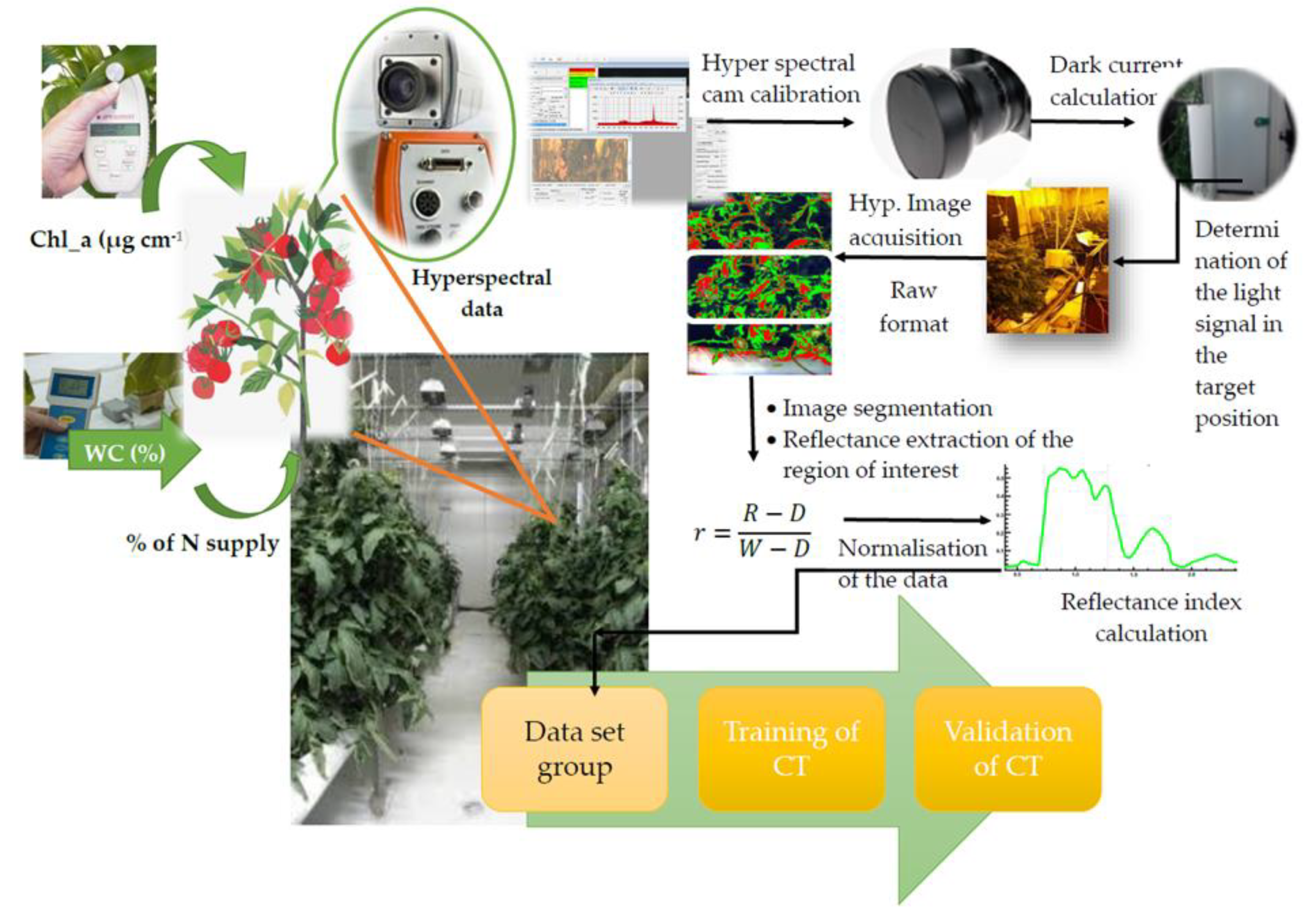
The radiation reflected by the plants were recorded with two spectra sensors: (1) a portable spectroradiometer (model ASD FieldSpec Pro, Analytical Spectral Devices, Boulder, CO, USA) and (2) a hyperspectral camera Imspec V10 (Spectral Imaging Ltd., Oulu, Finland). The spectroradiometer measures the radiation reflected in the range between 350 and 2500 nm, while the camera operates in the visible and near-infrared (VNIR) spectrum region between 400 and 1000 nm. The camera system was placed on a moving cart so that images of the vertical canopy axis could be obtained to cover the canopy area of young, fully developed leaves between the 3rd and 6th branches of three adjacent tomato plants. For extra illumination of the target area (70 × 100 cm), four quartz-halogen illuminators (500 W each) were used.

The system calibration procedures of both spectral sensors along with the method concerned the camera’s set up, image segmentation, and plant reflectance calculation was done as described in References [1,2,7,13,22]. The basic steps of the experimental setup are described in Figure 1.

2.3. Calculations

Based on the available reflectance measurements, the following indices (based on the analysis performed in References [1,7,13]) were calculated and evaluated to train the models:

PRI = (R₅₃₁ − R₅₇₀)/(R₅₃₁ + R₅₇₀)

(1)

TCARI = 3 × [(R₇₀₀ − R₆₇₀) − 0.2 × (R₇₀₀ − R₅₅₀) × (R₇₀₀/R₆₇₀)]

(2)

mrNDVI = (R₇₅₀ − R₇₀₅)/(R₇₅₀ + R₇₀₅ − 2 × R₄₄₅)

(3)

mrSRI = (R₇₅₀ − R₄₄₅)/(R₇₀₅ − R₄₄₅)

(4)

MSAVI = 1/2 × (2 × (R₈₁₀ + 1) − (√(2 × R₈₁₀ + 1) × 2 − 8 × (R₈₁₀ − R₆₉₀))]

(5)

OSAVI = (1 + 0.16) × (R₈₀₀ − R₆₇₀)/(R₈₀₀ + R₆₇₀ + 0.16)

(6)

where R is the reflectance value performed in each band expressed in nm that is indicated by the subscript number, mrSRI is the Modified red simple ration index and OSAVI is the Optimised soil-adjusted vegetation index.

2.4. Statistical Analysis

A classification tree was performed using SPSS (Statistical Package for the Social Sciences, IBM, USA) to create a tree-based prediction model of future irrigation events. Based on CT methodology, three hypotheses based on RI prediction rules were used to predict (i) the plant chlorophyll_a content (1st Hypothesis); (ii) the substrate water content (2nd Hypothesis), and (iii) to identify healthy, water- and nitrogen-deficit stressed plants (3rd Hypothesis). Each hypothesis independently consisted of structure trees, in which different RIs were involved. The CTs developed were based on the classification regression tree (CRT) and the chi-squared automatic interaction detection (CHAID) method to control the number of RIs and the maximum number of levels of growth beneath the root. The p-value was computed each time by applying Bonferroni adjustments. The method followed was done as described in References [13,23].

The models developed were calibrated (using training data) and validated (on a different set of data). A simple-sample validation was performed by using random assignment. A total of 75% of the total (n = 140 data sets) number of datasets were used as the training sample sets and 25% were used as the testing sample sets. The training sets were used to build the classification models, which were subsequently applied to the test set, which consisted of records with unknown class labels. The system tries to decrease the training error by completely fitting all the training examples. Each partition of each hypothesis was marked as the class label. During the 1st and 2nd Hypothesis, the class label was marked as Chl_a and θ (the numerical variable) and was expressed in μg cm⁻² and %, respectively, to predict the actual chorophyll_a and water status of the plant. To train the model, the measured Chl_a and θ values were considered as dependent variables.

During the 3rd Hypothesis, each partition was marked as either C (Control), WS (Water Stress), or NS (Nitrogen Stress) to answer the question if the crop is under water or nitrogen deficit stress. Thus, it could be considered that C referred to “no stressed plants/no irrigation or fertilization is needed”, WS referred to “water stress plants/irrigation is needed”, while NS referred to “nitrogen stress plants/nitrogen is needed”. The model was built according to substrate water and chlorophyll_a content evolution, in which θ values lower than 39% have been defined as WS. However, when the θ values were higher than 39%, while the Chl_a values were lower than 40 μg cm⁻², then the plant was defined as NS. These set points were derived from the analyses in References [1,7,13]. The algorithm employed a greedy strategy to grow the decision tree by making a series of locally optimum decisions about which attribute to use for the partitioning data. Each node of the training or testing samples showed the predicted value, which was the mean value for the dependent variable at that node. The mean value along with the measurement variability (standard deviation, ±SD) of the parameters measured are reported. The measure of the tree’s predictive accuracy was calculated based on a risk estimation and its standard error, where the proportion of cases were incorrectly classified after adjustment for prior probabilities and misclassification costs. The letter “n” is used to designate the daily sample size of each parameter. The goal of the classification models was to predict the class label of the unknown records. The current methodology followed the steps performed by Morgan [19], Loh [23], Lewis [24] and IBM SPSS Statistics 21 guide [25].

3. Results

3.1. Automation for Plant Chlorophyll_a Content Measuring

During the model analysis of the 1st Hypothesis where the Chl_a status of the tomato is predicted, two independently structured trees with different combinations of RIs (CT1 and CT2) were developed (Figure 2 and Figure 3). Both resulting structures consisted of eight nodes (two nodes with at least one child and four nodes without children). For each node, there is a table that provides the number (n) and the percentage (%) of Chl_a content cases in each reflectance index category set as a dependent variable.

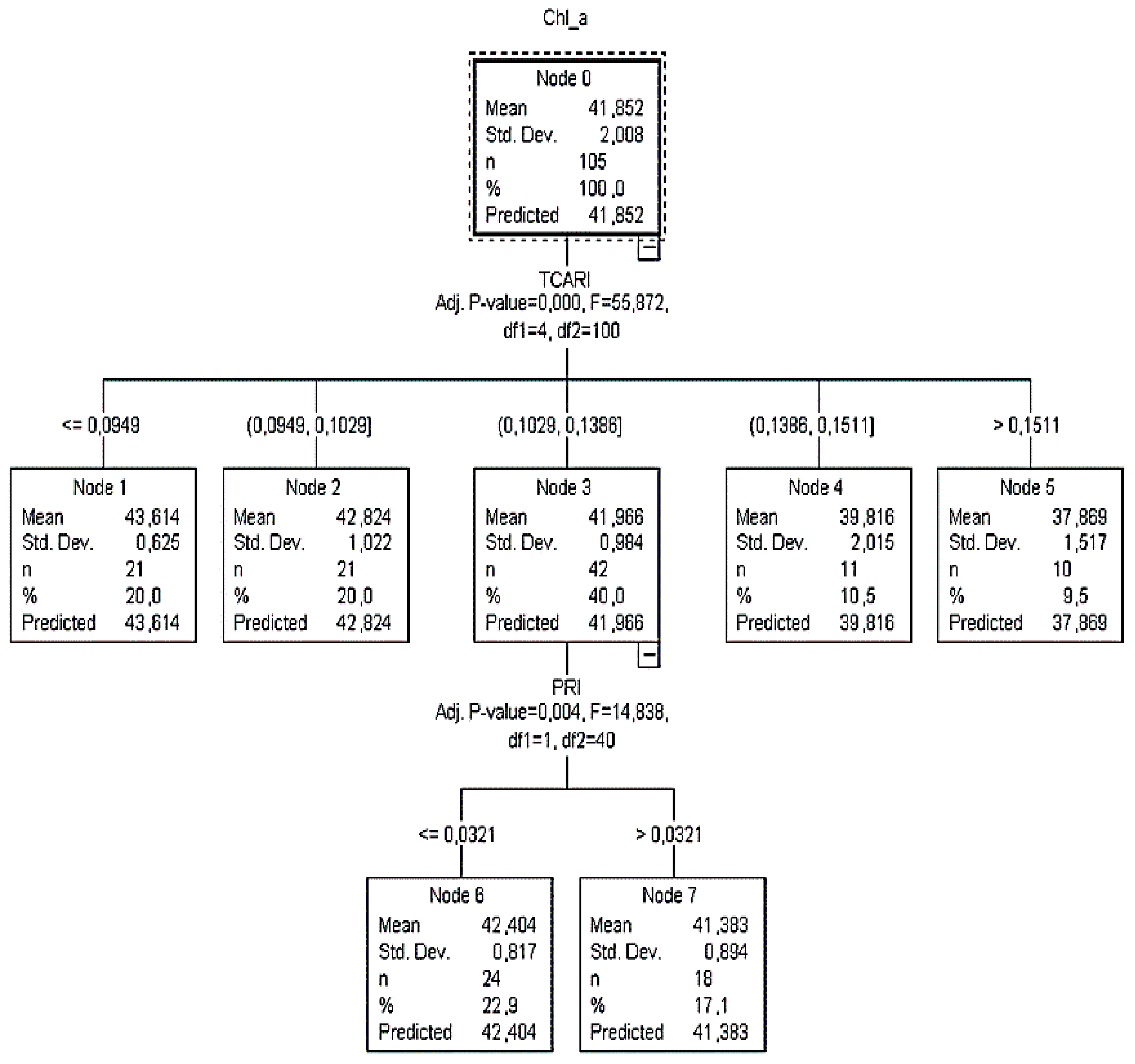
According to CT1, it was calculated that when TCARI was ≤0.0949, then the Chl_a content value was more than 43.61 μg cm⁻² (Figure 2). Additionally, when the TCARI ranged between 0.0949 and 0.1029, the Chl_a content varied close to 42.82 μg cm⁻² (SD = ±1). Since there were no child nodes below it, this was considered as the terminal node.

On the other hand, if the TCARI varied between 0.1029 and 0.1386, the PRI readings (next best predictor) had to be taken into consideration to identify the plant chlorophyll status and that node three was to be omitted. In this case, when PRI readings were ≤0.0321, 23% of the sample returned Chl_a equal to 42.4 μg cm⁻² (SD = ±0.8), otherwise (PRI > 0.03), 17% of the sample returned Chl_a equal to 41.4 μg cm⁻² (SD = ±0.9). For TCARI readings between 0.14 and 0.15 (node 4) and >0.15 (node 5), Chl_a was equal to 39.8 μg cm⁻² (SD = ±2.0) and 37.9 μg cm⁻² (SD = ±1.5), respectively.

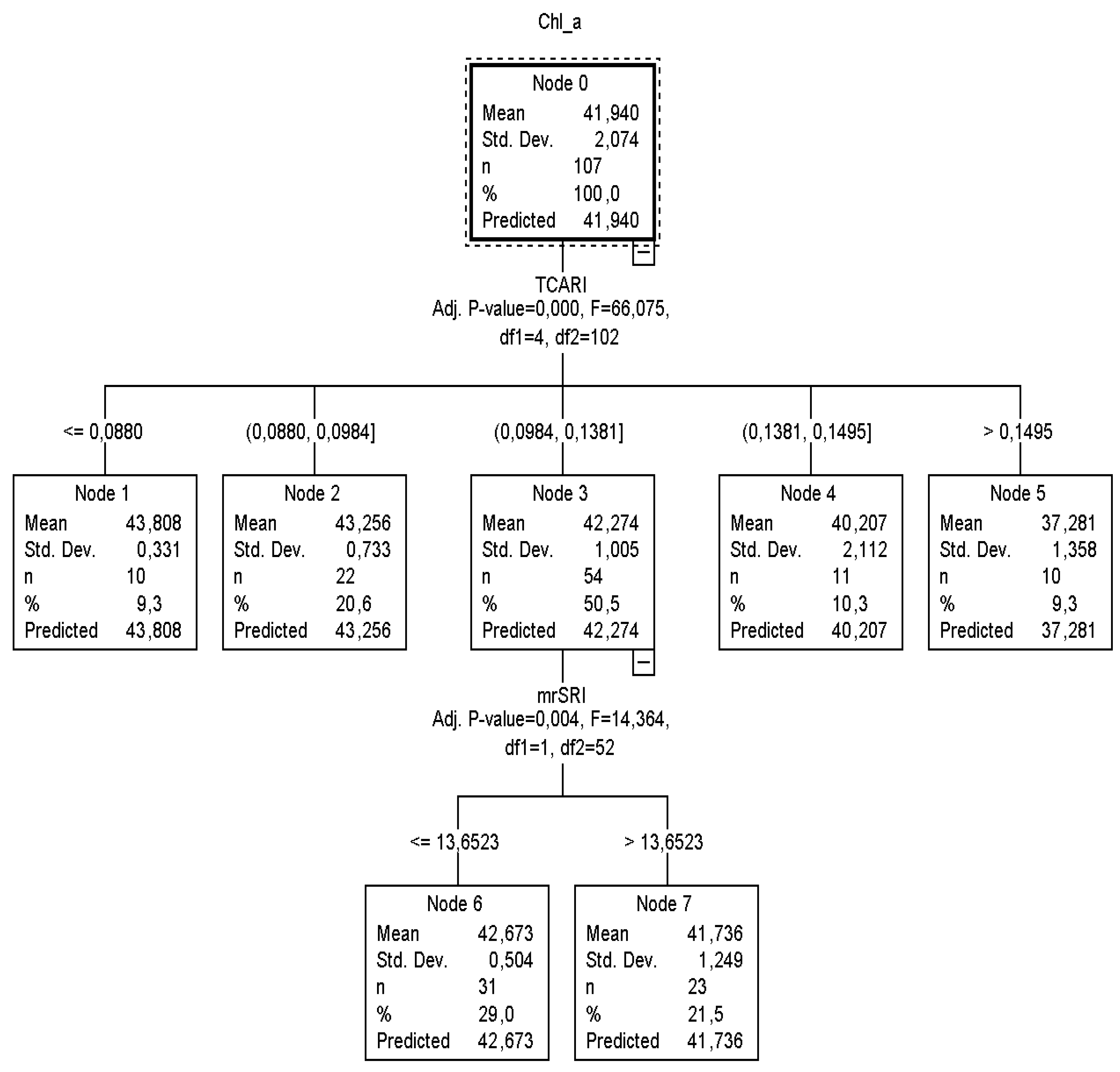
According to CT2 (Figure 3), it was calculated that when TCARI was ≤0.0880 and between 0.0880 and 0.0984, then nodes 1 and 2 returned similar Chl_a content values to CT1. On the other hand, if the TCARI varied between 0.0984 and 0.1381, the mrSRI readings (next best predictor) had to be taken into consideration to identify the plant chlorophyll status and that node three was to be omitted. In this case, when mrSRI readings were ≤13.6523, 29% of the sample returned Chl_a equal to 42.67 μg cm⁻² (SD = ±0.4), otherwise (mrSRI > 13.6523) 21.5% of the sample returned Chl_a equal to 41.73 μg cm⁻² (SD = ±0.9).

Both CT1 and CT2 structures did, however, reveal one potential problem with this model: for the plants that had a low level of Chl_a content, the standard deviation was high (>±1.0), which means that the data were widely spread and more than 20% of the predicted percentage inaccurately classified the Chl_a values lower than 39.8 μg cm⁻². This was also confirmed by the relevant node of the testing classification trees, where the SD was more than ±2. A comparison of the two structures, however, revealed that both CT1 and CT2 had a low estimation risk degree equal to 1.1. The trees resulting from the validation dataset provided an estimation risk degree equal to those of the training dataset (1.5 and 1.7, respectively).

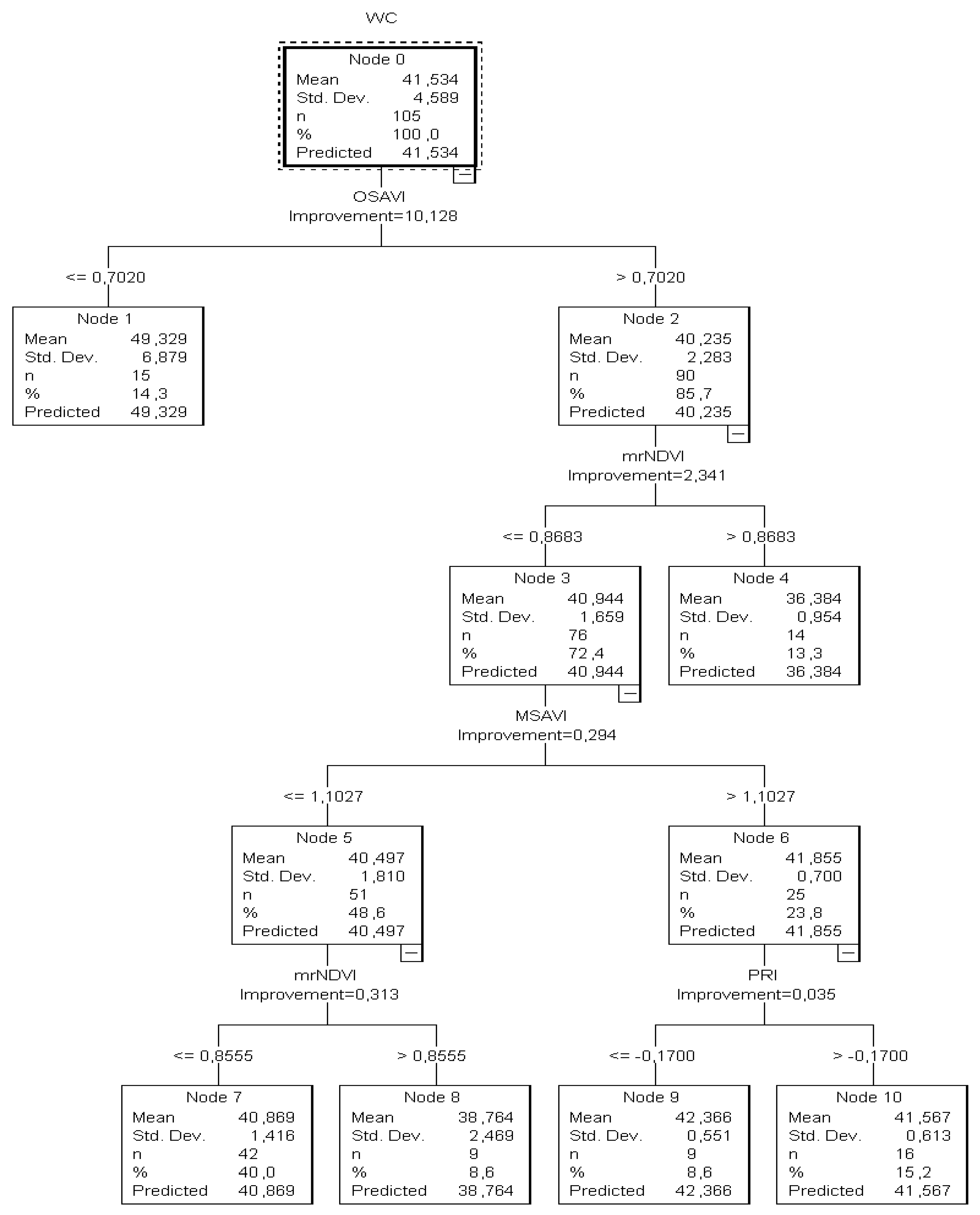
3.2. Automation for Substrate Water Content Measuring

In the 2nd Hypothesis, the tree (CT3) developed from both the training and testing samples had eleven nodes (five nodes with at least one child and six nodes without children) (Figure 4). In this tree, the predicted category was the estimation of the substrate water content (varied from 54.81 to 35%).

It was calculated that when OSAVI (a starter index) was ≤0.70, the tree returned the θ value as > 49.33%. Since there were no child nodes below it, this was considered the terminal node.

On the other hand, if the OSAVI was higher than 0.7020, the mrNDVI readings (next best predictor) had to be taken into consideration to estimate the substrate water status and that node two was to be omitted. In this case, when mrNDVI readings were ≤0.8683, the sample of the plants returned θ as equal to “36.38%” (13.3%) and the node was considered terminal as no child node developed below. However, by contrast, when mrNDVI was less than 0.8683, a combination of MSAVI and PRI readings had to be taken into account to estimate the substrate water content. This was also confirmed by the relevant node of the testing classification tree. However, the classification tree developed from the training data revealed a high estimation risk degree (7.06), while the risk degree in the tree based on the validation dataset was high as well (5.4). The high values of the risk estimation indicated that the accuracy of this structure was uncertain due to the θ values’ estimation and that more water content values should be included. The goal was to reduce the risk values to around 1.

3.3. Automation for Water and Nitrogen Deficit Stress Detection

During the model analysis of the 3rd Hypothesis, two independently structured trees with different combinations of RIs (CT4 and CT5) were developed (Figure 5 and Figure 6). CT4 consisted of nine nodes (four nodes with at least one child and five nodes without children) and CT5 of seven nodes (three nodes with at least one child and four nodes without children). In those trees, the predicted category was the detection of water and nitrogen deficit stress (C or WS or NS). For each node, the mentioned table provides the number (n) and the percentage (%) of the C or WS or NS cases in each reflectance index category set as a dependent variable.

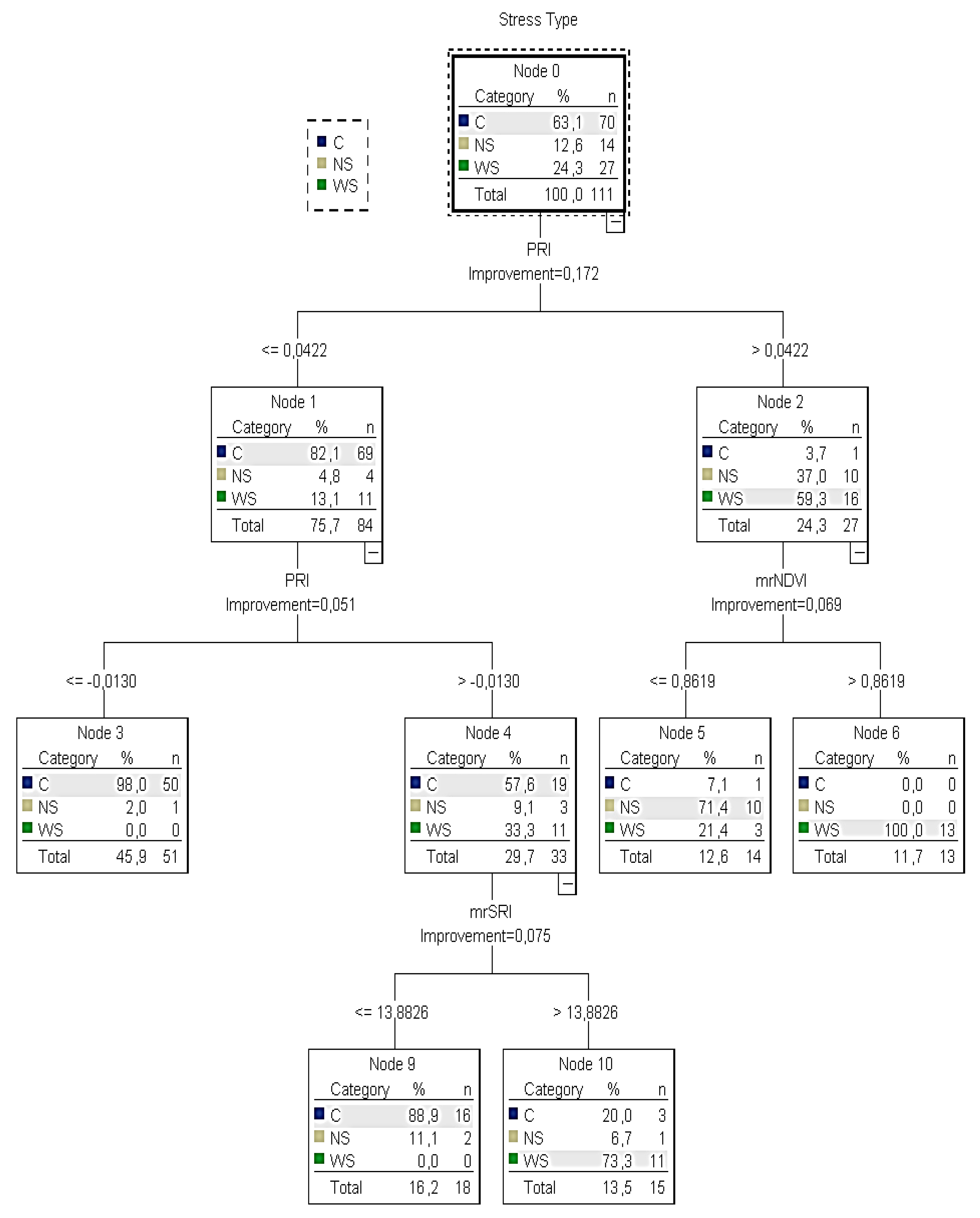
According to the training CT4 (Figure 5), it was calculated that there was no water or nitrogen deficit stress when PRI was ≤−0.0130 and C was returned (no irrigation is needed). On the other hand, if the PRI was between −0.01 and 0.04, the mrSRI readings (next best predictor) had to be taken into consideration to identify the water stressed plants and that node 4 was omitted. In this case, when mrSRI readings were ≤14, C was returned (no irrigation is needed). However, when mrSRI readings were >14, the majority of the sample (73%) returned WS. If the PRI was higher than 0.04, the mrNDVI readings (next best predictor) had to be taken into account. In this case, when mrNDVI readings were ≤0.86, NS was returned (nitrogen is needed). However, when mrNDVI readings were >0.86, the sample returned WS (irrigation is needed). However, contrary to node five of the training tree, in the testing tree, it was not clear when the plants were under water or nitrogen deficit stress because the sample of plants returning NS (60%) was very close to those returning WC (40%).

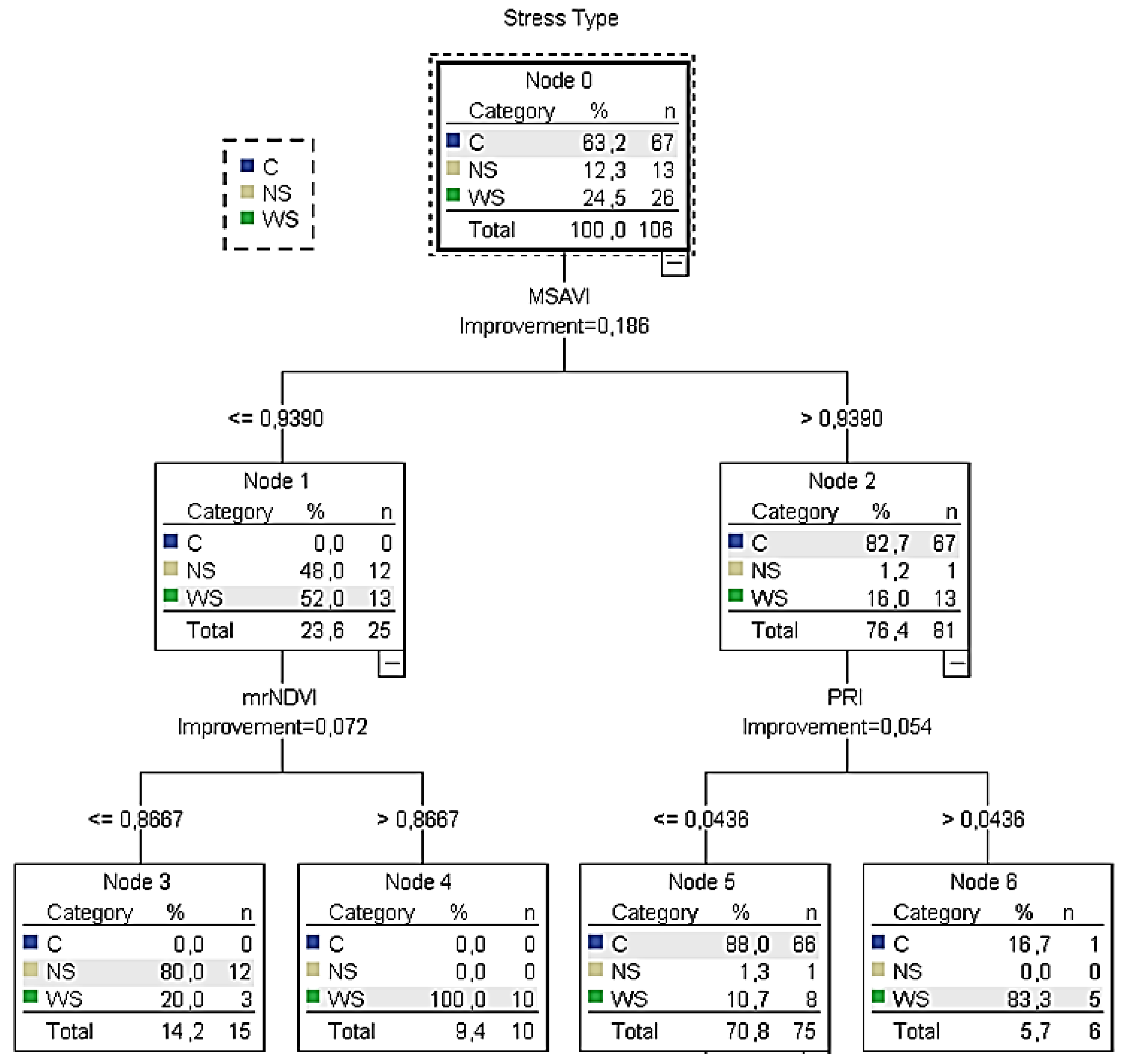
According to the training CT5 (Figure 6), it was calculated that when the MSAVI was lower than 0.94, the mrNDVI readings (next best predictor) had to be taken into consideration. In this case, when the mrNDVI readings were ≤0.87, the majority of the sample (80%) returned NS. On the other hand, when mrNDVI was higher than 0.87, the total sample was characterised as water stressed (irrigation is needed). On the other hand, if MSAVI readings were higher than 0.94, the PRI readings (next best predictor) had to be taken into consideration. In this case, when PRI readings were ≤0.04 and C was returned (no irrigation is needed). However, when PRI readings were >0.04, the sample returned WS (irrigation is needed). Similar results were confirmed by the relevant node of the testing classification tree.

Table 1. The classification accuracy of the training and testing sample for calibration and validation, respectively. C: control plants; WS: water deficit stress plants; NS: nitrogen deficit stress plants.

Classification Model	Sample	Observed	Predicted
			C	NS	WS	Percent Correct
CT4	Training CT4	C	66	1	3	94.3%
		NS	3	10	1	71.4%
		WS	0	3	24	88.9.7%
		Overall Percentage	62.2%	12.6%	25.2%	90.1%
	Validation	C	23	2	4	83.3.3%
		NS	0	2	1	75.0%
		WS	1	1	3	62.5%
		Overall Percentage	64.9%	13.5%	21,6%	76.7%
CT5	Training	C	61	0	6	91.0%
		NS	1	12	0	92.3%
		WS	1	3	22	84.6%
		Overall Percentage	59.4%	14.2%	26.4%	89.6%
	Validation	C	20	0	1	95.2%
		NS	1	3	1	60.0%
		WS	0	0	9	100.0%
		Overall Percentage	60.0%	8.6%	23.5%	91.4%

presents the number of cases classified correctly and incorrectly for each category of the dependent variable. The predicted percent of the training sample was 90.1% in CT4 and 89.6% in CT5, indicating that the model classified approximately 90.1% and 89.6%, respectively, of the sample correctly. Although the predicted percent of both CT4 and CT5 was similar, the CT4 result revealed one potential problem with this model: for those plants cultivated under nitrogen stress, NS was predicted for 71.4% of them, which means that 28.6% of the stressed plants were inaccurately classified with C (non-stressed plants) or WS (water stressed plants). On the other hand, only 5.7% of non-stressed plants were inaccurately classified as WS or NS stressed plants. However, the final estimation risk of the misclassification of the training model was low, with small differences between the two models reflected at 9% and 10%, respectively.

4. Discussion

Despite many statistical and mathematical models such as principal component analysis [17], artificial neural network, and other classification procedures that have been developed to extract optimal information from remotely sensed data, Yohannes and Hoddinott [26] and Camdeviren et al. [27] believed that the CT method was a very useful model for analysing complex datasets by providing visual results. Goel et al. [18] applied a classification tree method to group hyperspectral data in order to identify weed stress and nitrogen status of corn and compared it with artificial neural networks. The advantages of tree-based classification are that it does not require the assumption of a probability distribution, specific interactions can be detected without previous inclusion in the model, non-homogeneity can be taken into account, mixed data types can be used, and dimension reduction of hyperspectral datasets is facilitated [28].

In the current study, in order to determine the water and nitrogen deficit stress severity, reflectance indices were investigated in the CT paths. Among the indices, the CT model selected (MSAVI) as a starter index to predict the water and nitrogen deficit stress. The CT analysis revealed that the classification accuracy for the training sample was 89.6% and the testing tree responded to the predicted expectation by approximately 91.4%.

The overall success rate of classification accuracy between the predicted and measured values of the stressed tomato indicated that the combination of MSAVI, mrNDVI, and PRI has the potential to determine water and nitrogen deficit stress and that classification tree algorithms have good potential in the classification of remotely sensed spectral data. Elvanidi et al. [13] also reveal mrNDVI and PRI in the CT path to determine water deficit stress in tomato plants, with classification accuracy values of 84.2% and 78.9% for the training and testing sample, respectively. Additionally, Genc et al. [17] also tested the ability of the classification tree algorithm to assess water stress in corn using hyperspectral reflectance spectra transformed into spectral vegetation indices. Their results demonstrated that water and nitrogen stress in corn was detectable through spectral reflectance analysis.

Generally, the use of machine learning models is not widespread in agriculture since they require a long time-series of datasets. The destructive methods or the complex sensors used in the last decades to quantify plant physiology did not allow for their progress. With the recent integration of a new age of computational intelligent sensors, more and more robust methodologies are being adapted. Up to now, less than 40 articles focused on machine learning models in agriculture. From those, 61% of the articles were related to different aspects of crop management [29].

However, the prediction performed by those models, in most cases, mostly correspond specifically to the area and conditions used in the training data, thereby trying to account for the otherwise invisible variations specific to that land and surroundings [30]. In the open field, for instance, the terrain in which the crop is cultivated affects the process of the crop water demand prediction. With the advent of the new era of computational intelligent sensors that can track various things that were previously not possible, more and more factors can be considered. Nevertheless, this new concept will ensure the development of more robust remote sensing approaches for monitoring plant physiology in order to train a decision support system with the aim of adjusting climate and irrigation control strategies within the greenhouse. Thus, in the future, the widespread usage of machine learning models is expected, allowing for the possibility of integrated and applicable tools. However, improvement in the performance of the decision tree classification approach with increases in the number of data sets further strengthens the belief that, by increasing the amount of data, model performance could probably be further improved.

5. Conclusions

In the current work, the ability to use a classification tree was tested to remotely predict leaf chlorophyll and substrate water content. Additionally, the classification tree was trained to assess different types of tomato stress such as water and nitrogen deficit stress. The model was trained by organizing, in the most effective way, the reflectance values measured by a hyperspectral camera. Among the reflectance indices, the classification tree model selected TCARI and PRI or mrSRI to predict leaf chlorophyll content. To estimate the substrate water content, on the other hand, the process was much more complex since more than four reflectance indices were involved in the procedure. Regarding the model trained to sense the actual plant water and nitrogen status, it was concluded that the combination of MSAVI, mrNDVI, and PRI involved in CT5 made insufficient provision with a reasonable accuracy. These results are promising for designing a smart decision support system for better managing climate and irrigation control strategies. Additionally, less complicated reflectance sensors recording certain spectral bands could be adapted to monitor plant physiology in real-time in a cost-effective manner. Nevertheless, it has to be noted that the results presented are relevant to the conditions of the measurements and the specific crop studied. Therefore, it is expected that the use of machine learning models will be even more widespread in the near future.