Article

Comparative Effects of Nitrogen Fertigation and Granular Fertilizer Application on Pepper Yield and Soil GHGs Emissions

1
Institute for Agriculture and Forestry Systems in the Mediterranean (ISAFoM), National Research Council of Italy, P. le Enrico Fermi 1, Loc. Porto del Granatello, Portici, 80055 Naples, Italy
2
Institute for the Animal Production System in the Mediterranean Environment (ISPAAM), National Research Council of Italy, P. le Enrico Fermi 1, Loc. Porto del Granatello, Portici, 80055 Naples, Italy
3
Institute of Biosciences and Bioresources (IBBR), National Research Council of Italy, Research Division Portici, Via Università 133, Portici, 80055 Naples, Italy
*
Author to whom correspondence should be addressed.
Horticulturae 2025, 11(6), 708; https://doi.org/10.3390/horticulturae11060708
Submission received: 21 May 2025 / Revised: 14 June 2025 / Accepted: 16 June 2025 / Published: 19 June 2025
(This article belongs to the Section Plant Nutrition)

Abstract

:
Quantitative greenhouse gas (GHG) budgets for Mediterranean pepper cultivation are still missing, limiting evidence-based nitrogen management. Furthermore, mitigation value of fertigation respect to granular fertilization in vegetable systems remains uncertain. This study therefore compared the GHG footprint and productivity of ‘papaccella’ pepper under two nitrogen fertilization methods: granular fertilization versus low-frequency fertigation with urea, each supplying about 63 kg N ha−1. Eight automated static chambers coupled to a cavity ring-down spectrometer monitored soil CO2 and N2O fluxes throughout the season. Cumulative emissions did not differ between treatments (CO2: 811 ± 6 g m−2 vs. 881 ± 4 g m−2; N2O: 0.038 ± 0.008 g m−2 vs. 0.041 ± 0.015 g m−2, fertigation vs. granular), and marketable yield remained at ~11 t ha−1, leaving product-scaled global warming potential (GWP) unchanged. Although representing less than 2% of measured fluxes, “hot moments,” burst emissions exceeding four standard deviations (SD) from the mean, accounted for up to 4% of seasonal CO2 and 19% of N2O. Fertigation doubled the frequency of these events but reduced their peak magnitude, whereas granular application produced fewer but more extreme bursts (>11 SD). Results showed that fertigation did not mitigate GHGs emission nor improve productivity for Mediterranean pepper, mainly due to the low application frequency and the use of a urea fertilizer. Moreover, we can highlight that in horticultural systems, omitting ‘hot moments’ leads to systematic underestimation of emissions.

Graphical Abstract

1. Introduction

Arable lands significantly contribute to atmospheric pollution through greenhouse gases (GHGs) [1], which are released from soils and influenced by crop managing practices such as soil tillage and fertilization [2]. Nitrous oxide (N2O) has about 300 times higher global warming potential (GWP) than carbon dioxide (CO2) and contributes approximately 6.2% to anthropogenic global warming [3].
N2O is produced through nitrification and denitrification, both influenced by nitrogen (N) fertilization and affected by soil oxygen, water content, pH, temperature, and N and C availability [4,5,6]. Nitrogen fertilization plus irrigation increases yields needed to meet global food demand [7,8,9] but is also the main cause of N2O production in agroecosystems [10]; it is usually applied early as synthetic or organic granular fertilizer. Early season dry granular application, when plant uptake is low, increases soil N losses as N2O because of high N availability for N2O-producing microbes [11,12]. Fertilizer transport depends on soil texture, moisture, and concentration, complicating infiltration and promoting leaching if mismanaged [13,14,15]. Soil–water relations and GHGs production are coupled. Soil porosity controls moisture and nutrient distribution [16,17,18] and irrigation that alters the moisture regime can raise N2O emissions by 50–140% [19,20]; thus, fertilization and water management affect emissions by modifying soil properties and microbial communities, the main N2O drivers [6].
Fertigation, the delivery of dissolved N fertilizers through irrigation water [21,22,23,24], transports nutrients directly to roots [25,26] and enables precise N management [27], uniform distribution and lower N availability for N2O-producing microorganisms [28,29]; however, repeated N-and-water pulses can amplify N2O. A meta-analysis of 139 field studies showed consistent yield gains but highly variable N2O responses, leaving the climate benefit uncertain [30]. Emission reductions of 25–50% occurred in drip-fertigated tomato, cucumber and celery versus furrow or flood irrigation [8,31,32], whereas fertigation in northern China showed no N2O mitigation and even reduced maize yield compared with drip [22] and flood irrigation [33], and emissions tripled in a Californian almond orchard versus micro-sprinklers [34].
Efficiency depends on application frequency and N form: ammonium or urea generally produce more N2O than nitrate [35,36,37]; high-frequency (HF) ammonium fertigation in almond did not reduce N2O versus low-frequency (LF), whereas HF nitrate fertigation did [38]; in Spanish melon, drip fertigation with urea emitted 2.4 times more N2O than calcium nitrate, and HF increased CO2 by 21% [39]; subsurface HF fertigation in greenhouse Chinese cabbage increased cumulative N2O while leaving CO2 unchanged and increasing yields by 45.1–49.2% versus LF [40].
Assessing these interactions requires high-resolution monitoring; low-frequency manual chambers miss “hot moments” and “hot spots” that dominate annual N2O emissions [41,42,43,44,45,46,47]. Such events are triggered by rainfall, freezing or management practices [46,48,49,50,51], related to soil moisture, oxygen, temperature, and nitrate availability [48], and often occur where litter and land-use legacy are high [47,52,53], accounting for large annual shares within days to weeks [45,46,47,54,55]. Hot moments exceed 4 standard deviations (SDs) above the mean (99.9th percentile) [54]; treating them as outliers [56] can ignore key processes [57,58]. Long-term high-frequency N2O monitoring remains rare; most CRDS-automated chamber setups use only 6–12 chambers, limiting coverage [59,60,61].
Pepper (Capsicum annuum L.) “papaccella”, a high-N vegetable symbol of Campania and widely used in Neapolitan cuisine, is among the world’s most cultivated vegetables [62,63]. In Mediterranean nitrate-rich soils, irrigation can double N2O versus rain-fed fields, making strict N management essential [64,65]. Although fertigation can raise yield and mitigate N losses in semi-arid Mediterranean systems [30], its GHGs impact on pepper is poorly studied; evidence for Mediterranean pepper is limited [40] and most data come from Asia and America [65,66], while hot-moment dynamics under Mediterranean fertigation remain unexplored. Insufficient knowledge on optimized N rates, fertilizer selection and irrigation can make fertigation more N2O-emitting than conventional systems.
To address these knowledge gaps, we investigated how fertigation influences pepper yield, GHG emissions, and the dynamics of “hot moments “emissions in a Mediterranean cropping system. The specific objectives were to (1) compare fertigation with conventional granular fertilization in terms of CO2 and N2O fluxes and pepper yield and (2) quantify the contribution of the captured hot moments to the cumulative fluxes in each treatment, thereby assessing their impact on total emissions. We hypothesize that fertigation reduces GHGs emissions while maintaining crop yield. Furthermore, we also hypothesized that hot moments drive to higher fluxes for both treatments and that the enhanced soil water content in the fertigated plots would lead to both higher frequency and quantitative contribute of N2O hot moments.

2. Materials and Methods

2.1. Trial Materials and Experimental Design

The trial was carried out at an experimental site near Naples (Acerra, Italy, 40°57′ N, 14°25′ E) equipped with a meteorological station managed by the Campania region (https://agricoltura.regione.campania.it/meteo/dati_2023/acerra_2023.html, accessed on 14 December 2024), located in a field very close to the experimental site (about 100 m, Figure S1). The experimental site is characterized by Mediterranean climate (Figure 1A,B) and coarse soil texture (Table S1).
Plants of sweet pepper (Capsicum annuum L., cv. “Papaccella”) were transplanted on 30 May 2023, at a spacing 1.0 m × 0.4 m. Therefore, a plant density of 2.5 plant per m2 was obtained. Each plot had a size of 30.4 m2. All seeds were supplied by the regional vegetable germplasm bank of Campania (Banca del Germoplasma Orticolo della Regione Campania, Italy).
Two treatments in four replicates were tested and compared: nitrogen fertilization as urea was supplied to crops either as granular fertilizer (G) or in fertigation (F). Urea was supplied in fertigation at 36, 50, 65, 80, and 98 days after transplanting (DATs) by dissolving it in irrigation water, whereas the granular fertilizer was applied at 36, 65, and 98 DATs. According to the pepper cultivation protocol of the Campania Region [67] and based on soil analyses performed, the nitrogen requirement was estimated at 63.5 kg N ha−1. The distribution of nitrogen via granular fertilization followed local agronomic practices and was carried out in three key phenological stages of the plant. In details, 20% of the total dose was applied one month after transplanting. The 40% was supply at post-fruit set phase, the last 40% was delivered at the onset of maturation, about one month after the previous fertilization. The fertilizer, composed of urea (Fertilsud, Spinazzola, BT, Italy), was applied within the root development area of the plants. Fertigation was also performed according to commonly adopted local procedures. The fertilizer was supplied every fifteen days for a total of five applications. The first two applications each supplied 10% of the total nitrogen dose, while the following three applications each provided approximately 26.5%.
Plants were irrigated using a subsurface drip irrigation system (Antisiphon technology). Drip lines were buried approximately 20 cm below the soil surface, aligned along the crop rows. Emitters were spaced at 10 cm intervals, with a flow rate of 2.13 L/h, following the same scheduling for both treatments. Irrigation was applied with frequency of about three days (Figure 1A). The water volume was estimated according to the crop’s needs. Irrigation of each plot was independent. To ensure proper fertilizer distribution during fertigation applications, considering the plot area, the fertilizer was dissolved in an agricultural tank equipped with a mixer. Once dissolved, the fertilizer was injected directly into the drip lines. The dosing unit was the plot, consisting of approximately 72 plants over an area of 30 m2. For the first two applications, 48 g of fertilizer per plot (approximately 0.54 g per plant) were dissolved in 100 L of water. From the third to the fifth application, 104 g of fertilizer per plot were dissolved in 100 L of water for each application. Weeds were manually removed throughout the whole crop growing season.

2.2. Biometrical Determinations

The plant dry biomass production was monitored five times during the whole crop growing season. Two plants per plot were sampled, portioned into root, stem, leaves and fruits, and dried in oven at 65 °C up to a constant weight [68]. Fruits were harvested during the reproductive phase of crop as the product became marketable (i.e., redness of 50% of the fruit surface) and the cumulative yield from these harvests was used to calculate the yield-scaled global warming potential (GWP/Y).

2.3. Automated Chamber Greenhouse Gases Fluxes Measurements

Soil greenhouse gases fluxes of CO2 and N2O, continuously monitored from 29 June 2023 to 17 September 2023, were measured using an automated chamber system, consisting in a Picarro G2508 cavity ring-down spectrometer (CRDS) (Picarro, Santa Clara, CA, USA) [69] connected via an eosMX multiplexer (Eosense Inc., Dartmouth, NS, Canada) to 8 eosAC automated chambers (Eosense Inc., Dartmouth, NS, Canada) [61,70], in order to assess the small-scale spatial variability. The multiplexer allowed for sequential chamber deployment and directed gases to the CRDS analyzer. The Picarro G2508 operates with a 105 mL analytical cell, maintained at a constant pressure of 140 Torr and a temperature of 45 °C, ensuring stable conditions for gas quantification. The system consisted of a closed loop with a low-leak diaphragm A0702 pump (Picarro, Santa Clara, CA, USA) facilitating sample circulation, while a vacuum pump ensured continuous gas recirculation through the chamber headspace at a rate of 240 mL min−1 during the enclosure. Picarro analyzer allowed real-time in situ headspace gas concentration measurements, at a frequency of 1 Hz. Chambers were deployed in the field, atop collars made of Schedule 40 polyvinyl chloride (PVC) pipes with a diameter of 15.2 cm, inserted into the soil to an average depth of about 4 cm to minimize leakage and disturbance. Each chamber was connected to the multiplexer with 35 m of Teflon inlet tubing, 35 m of outlet inlet tubing and 35 m data cable. Each flux measurement lasted ~12 min, with a pre- and post-flushing period of 2 min to ensure gas exchange stabilization. This timing allowed to cover the high-frequency temporal variability, providing measurements of each gas at four time points throughout the day (00:00, 06:00, 12:00, 18:00 solar time). The total headspace of the automated chamber system was 3.07 L. The 8 eosAC automated chambers were divided into two groups of 4 chambers, in order to have 4 replicated measurements of each treatment.
Volumetric Soil Water Content (VSWC) and Soil Temperature (Ts) were measured in the proximity of each chamber, at the depth of 5 cm, using the soil sensor MAS-1 4–20 Milliamp Soil Moisture Sensor (METER Group, Pullman, WA, USA) and the RT-1 Soil Temperature Sensor METER Group, Pullman, WA, USA) for SWC and Ts, respectively. The Water-Filled Pore Space (WFPS) was calculated as follows: WFPS = VSWC/(1 − (BD/2.65)) where BD is the bulk density and 2.65 represents the average density calculated based on the relative content of the different mineral constituents.

2.4. Data Managing and Filtering

Flux calculations and fitting were performed using Eosense eosAnalyze-AC v3.9.11 software (Eosense Inc., Dartmouth, NS, Canada). All the data were recorded and processed with the Time Zone setting of UTC +1:00. Data quality assessment and filtering were conducted in R (RStudio, v4.3.3). CO2 fluxes were removed from the final dataset if R2 of the linear fitting function (gently implemented by Eosense in the Eosense eosAnalyze-AC software) was smaller than 0.8. N2O fluxes were removed if R2 of the linear fitting function was smaller than 0.7 but kept if CO2 fluxes passed the previous filter in the same sample. This data filtering removed 4.09% of the flux measurements. Following data filtering, to explore and evaluate the importance of the hot moments, we manipulated the dataset in order to acquire two versions of it: (i) raw data left untouched and (ii) a “cleaned” version where outlier’s removal was applied using the Interquartile Range (IQR) method as well as a gap filling with a mobile mean (window size = 3) in R (RStudio, v4.3.3). We adopted this approach keeping in mind that hot moments risk to be treated as outliers, since they show a significant drift from the mean distribution of the data, ignoring or underweighting this phenomenon [55,57,58]. Therefore, hot moments were defined as measurements which values were 4 standard deviations greater than the mean [54,55]. Hot moment frequency was estimated by calculating the percentage ratio among the actual number of measurement values exceeding the 4 standard deviations and the total recorded fluxes, for each gas for both treatments. Contextually, the percentage contribution of the hot moments to the total flux derived from the ratio between the total sum of the hot moments and the total sum of all recorded fluxes. The final dataset, without removing or transforming hot moments as they were outliers, was averaged on a daily basis. Furthermore, it was divided into six subperiods following the five fertigation dates (4 and 18 July, 2 and 17 August, 4 September), three of which matched the granular fertilization dates (4 July, 2 August, 4 September), plus the shorter period before the first fertilization date (period 1, DAT 31–35). For these subperiods a mean daily profile was computed, averaging all the measurements in the same hour (00:00, 06:00, 12:00, 18:00) across each subperiod, providing a representative daily pattern of each variable (CO2, N2O, Ts, and WFPS), in order to explore the temporal variability during the season. Cumulated emissions of CO2 and N2O were calculated using the trapezoid rule [60,71]. To calculate the environmental impact of crop management, we estimated the yield-scaled GWP (kg CO2-eq kg−1 yield) following the IPCC AR5 100-year GWP value of 298 CO2-eq for N2O [72].

2.5. Statistical Analysis

All statistical analyses were performed using SPSS software (v. 29.0.1.0, IBM, Chicago, IL, USA). Differences in daily average emissions of CO2 and N2O, Water-Filled Pore Space (WFPS), and Ts were assessed using Standard Error of the Mean (SEM). Differences in daily trends for CO2 and N2O fluxes, WFPS, and soil temperature across different experimental periods were analyzed using SEM and one-way ANOVA. Daily average fluxes of CO2 and N2O, with and without hot moments, were analyzed using SEM and a paired t-Test. Hot moments for each chamber were evaluated using standard deviation. The interaction among fertilization methods, CO2 and N2O emissions, soil temperature, and WFPS was analyzed through multiple linear regression.

3. Results

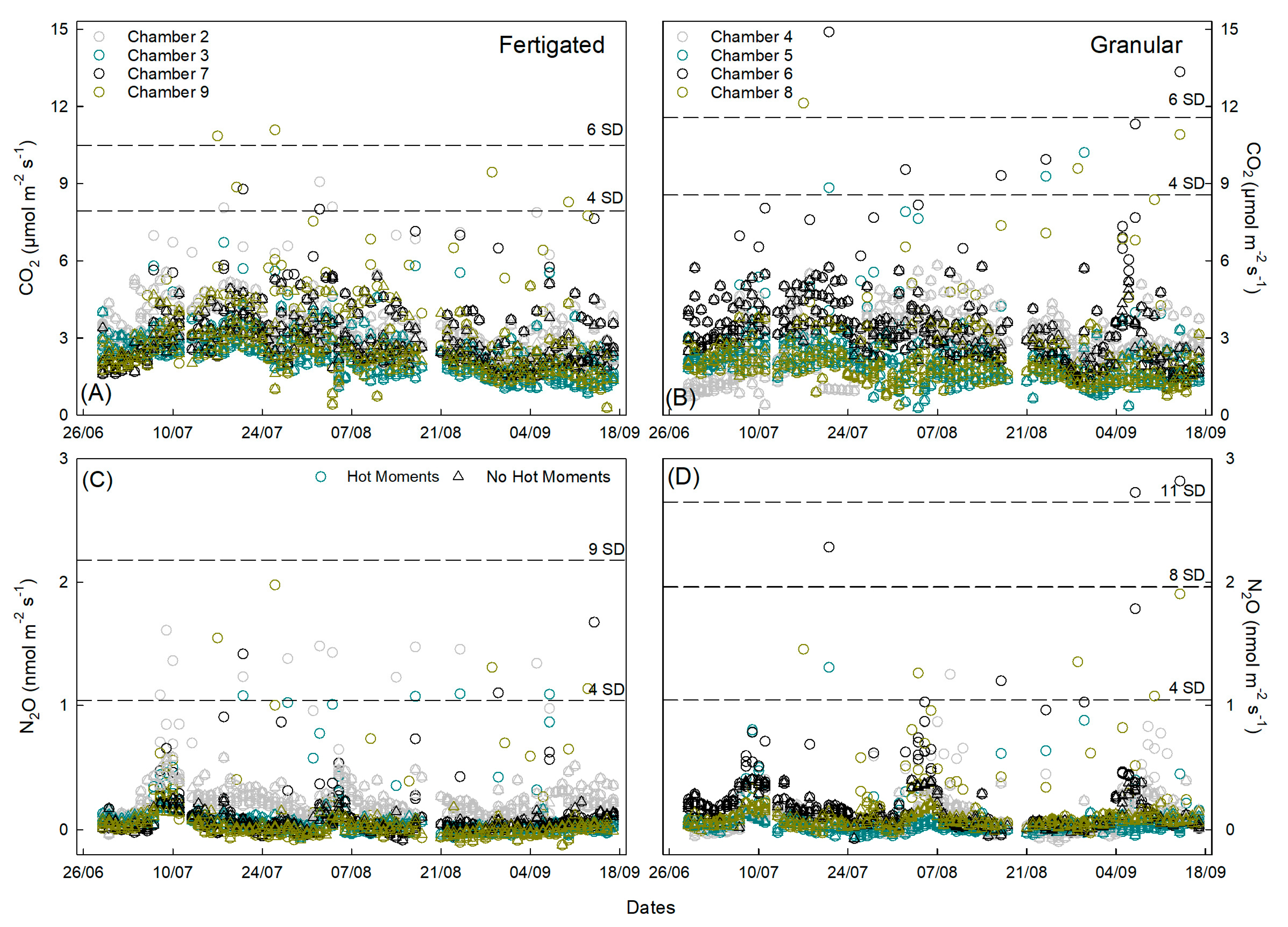
3.1. CO2 and N2O Daily Fluxes and Environmental Drivers over the Season

Over the whole experimental period, daily air temperature ranged from a minimum of 12.3 °C to a maximum of 39.6 °C, showing the same trend for all three months of the experiment (Figure 1A). Rainfall ranged from 0.2 to 2.6 mm, with a single intense event (12.6 mm) on 4 August (DAT 67), leading to a rapid drop in both minimum and maximum air temperature, which raised again after four days (Figure 1A,B).
Daily average GHGs fluxes show the onset of peak emissions after the first fertilizer application on 4 July (DAT 36), for both treatments (Figure 1C,D). Fertigation slightly increased CO2 emissions in the first month (DAT 36 to 64), where the first two fertigation (F) and the first granular fertilizer application (G) occurred, followed by a decrease in the fluxes. Mean CO2 flux was significantly higher in treatment F (2.88 ± 0.67 µmol m−2 s−1) than in treatment G (2.65 ± 0.55 µmol m−2 s−1; Table 1, p < 0.05).
The highest F treatment N2O peak (DAT 41; 0.5 ± 0.08 nmol m−2 s−1) was measured after the first fertigation, followed by the peaks measured after each fertigation event (DAT 53: 0.32 ± 0.11 nmol m−2 s−1; DAT 68: 0.34 ± 0.03 nmol m−2 s−1 and DAT 101: 0.33 ± 0.09 nmol m−2 s−1). G treatment N2O fluxes followed a similar pattern, with the highest peaks measured after the second granular application, when high fluxes lasted for three consecutive days (DAT 67–69; 0.38 ± 0.08, 0.37 ± 0.07, and 0.36 ± 0.06 nmol m−2 s−1), and the last granular application (DAT 101: 0.46 ± 0.18; DAT 108: 0.37 ± 0.20; Figure 1D).
In the fertigated treatment, WFPS accounted for a limited portion of the N2O flux variability (Table 2; R2 = 0.158, p < 0.05), with higher soil moisture levels coinciding with N2O emission peaks. In the granular treatment, N2O fluxes showed a weak correlation with both Ts and WFPS (Table 2; R2 = 0.045, p < 0.05). Ts for both treatments show a decreasing trend during all the measurement periods after the first month of irrigation and rapidly drop from 29 °C till 23 °C after the intense rain event on DAT 67 (Figure 1F). Ts showed a week relation with CO2 for the F treatment (Table 2; p < 0.05, R2 = 0.06). WFPS showed no relation to CO2 fluxes in the fertigated treatment; while this can explain a small portion of the observed variance for the G treatment, it is not statistically significant (R2 = 0.03; Table 2).
WFPS showed values around 30% at the beginning of the experiment for both treatments, with values smaller by up to 18% for the fertigated treatment and higher values for the F treatment (Figure 1E).
Both treatments showed transient N2O spikes shortly after fertilization (Figure 1D). The granular treatment averaged 0.12 ± 0.10 nmol m−2 s−1 versus 0.13 ± 0.10 nmol m−2 s−1 under fertigation, but this difference was not significant (Table 1).

3.2. CO2 and N2O Fluxes Diel Trends by Fertilization Period

GHGs diel periodic trends show the first period before the first fertilization (DAT 31–35; Figure 2A,G,M,S) where CO2 and N2O fluxes fluctuate at the background level, with the F treatment CO2 flux significantly higher early in the morning (Figure 2A; p < 0.05). Soil temperature reached the higher temperature in this period, peaking in the middle of the day (about 31 °C; Figure 2M), whereas WFPS was at a low level, ranging from 20 to 30%, with lower water content for the F treatment.
Period 2 (DAT 36–49; Figure 2B,H,N,T) was characterized by the first N fertilizer input, causing GHG peak emissions around midday (12:00). CO2 showed slightly higher fluxes in the F treatment from early morning to afternoon (Figure 2B; p < 0.05). N2O peaked in the middle of the day in the F treatment, with flux significantly higher than the G treatment (Figure 2H; p < 0.05). In this period, after the first irrigation and fertilization, WFPS started to increase (Figure 2T).
In the third period (DAT 50–64; Figure 2C,I,O,U) daily CO2 fluxes significantly increased in the fertigated treatment (Figure 2C; p < 0.05), reaching the highest peak of 4.41 ± 0.14 µmol m−2 s−1 at noon, whereas N2O emissions were quite similar between the two fertilizations, peaking early in the morning (Figure 2I), along with the temperature drop and WFPS increase (Figure 2O,U).
In period 4 (DAT 65–79; Figure 2D,J), both CO2 and N2O fluxes decreased in the F treatment, with N2O showing significant lower fluxes in the F treatment than the G treatment at noon (Figure 2J; p < 0.05). The WFPS daily trend of the F treatment was significantly higher (Figure 2V; p < 0.05), while Ts dropped early in the morning (Figure 2P).
In period 5 (DAT 80–97; Figure 2E,K,Q,W) CO2 fluxes showed no difference among the two treatments (Figure 2E), while N2O results were significantly higher in the F treatment (Figure 2K; p < 0.05). During this period WFPS continued to increase in both treatments, becoming significantly higher in the F treatment (Figure 2W; p < 0.05), reaching 41.2 ± 1.8% early in the morning.
The sixth and final period (DAT 98–111; Figure 2F,L,R,X), showed both CO2 and N2O fluxes with the same diel trend, slightly higher in the G treatment, without statistically significant differences (Figure 2F,L). Ts has decreased overall, with mean hourly values significantly differencing among the two treatments (Figure 2R; p < 0.05), while WFPS reached lower values, but was still significantly higher in the F treatment (Figure 2X; p < 0.05).

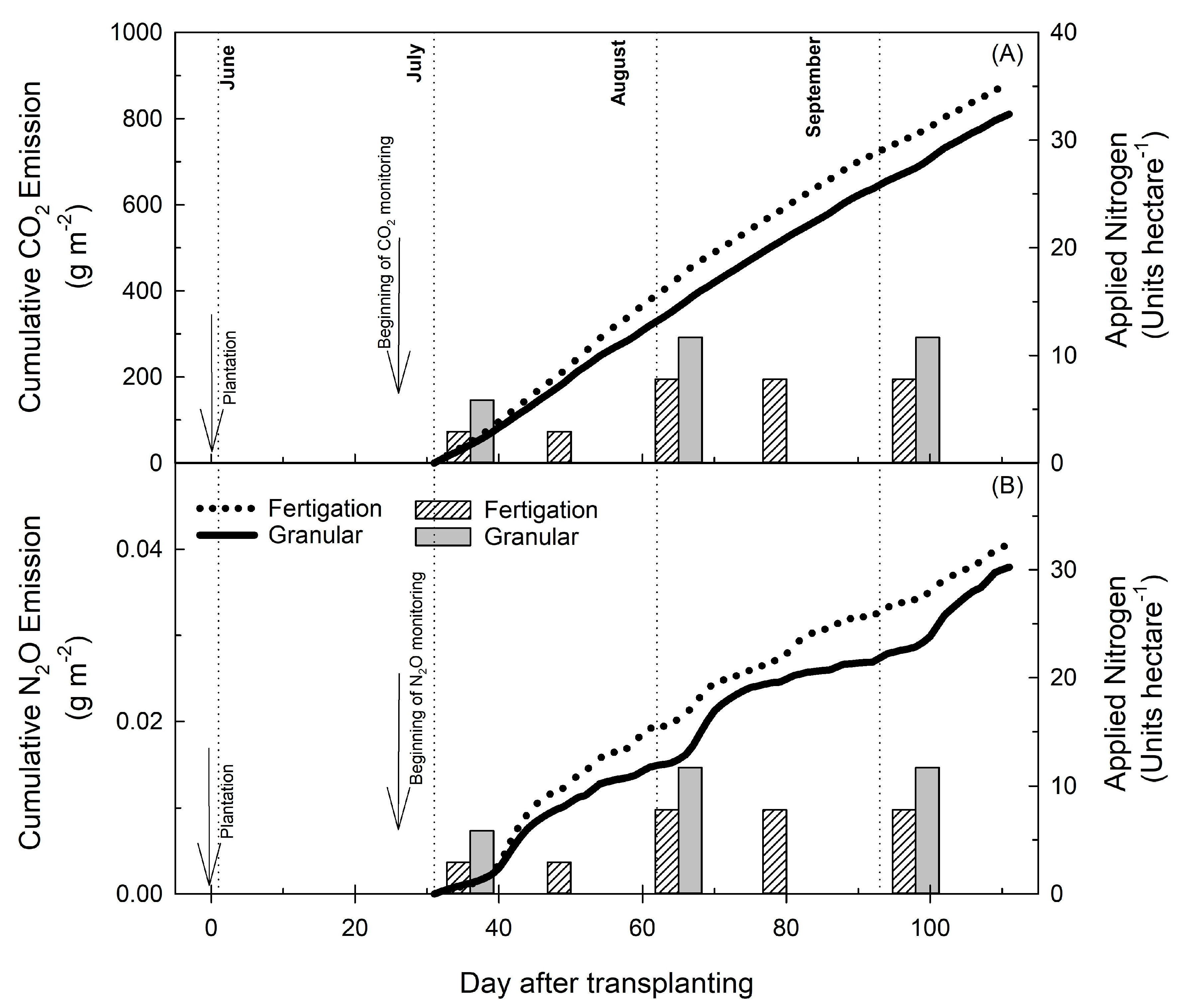
3.3. Growing Season Cumulative Fluxes and Yield-Scaled Global Warming Potential

Over the entire study CO2 cumulative emission from the fertigated treatment was 881 ± 113 g m−2, higher than the granular treatment emission of 811 ± 187 g m−2, even though not significantly different (Table 1). N2O cumulative emission was similar among the two treatments, 0.041 ± 0.03 and 0.038 ± 0.02 g m−2 for F and G treatment, respectively (Table 1). Cumulative emission started right after the first fertilizer application for both gases, while cumulative curves of the two treatments begin to separate after the second fertigation (Figure 3). CO2 and N2O daily cumulative emission remain slightly higher in the F treatment for the whole season, albeit not statistically significant (Figure 3). This study showed that neither fertigation nor granular fertilization reduced yield-scaled global warming potential (GWP/Y) for CO2 and N2O (Table 2), as well as pepper yield at the end of the season was similar between the two treatments, resulting in 11,075 and 11,325 kg ha−1 for F and G treatment, respectively.

3.4. Hot Moments Contribution Importance Across the Season

Across the two treatments no chamber was a source of hot moment emission consistently enough to be classified as hot spot, for both CO2 and N2O, even though the intra-season variability was largely driven by hot moment frequency and magnitude (Figure 4).
In the G treatment, the CO2 hot moments represented only 0.99% of the measured fluxes, but contributed to the mean flux rate by 4%, whereas in the F treatment, both frequency and contribution were smaller, at 0.82 and 2.6%, respectively (Table 1). In the G treatment CO2 hot moments reached the highest fluxes of the whole trial, at 12 and 15 µmol m−2 s−1, after 13 and 20 days from the first N input, respectively, and 13.34 µmol m−2 s−1 5 days after the last fertilizer application (Figure 3B). These hot moments were greater than 6 standard deviations. CO2 hot moments for the F treatment reached smaller values compared to the G treatment, barely exceeding the 6 standard deviations with the fluxes of 10.8 and 11.08 µmol m−2 s−1 (Figure 4A). N2O hot moments represented 0.99% of the measured fluxes for the G treatment, same as for CO2, and 1.88% for the F treatment, with the contribution to the mean flux rate about 3 times higher than CO2, at 13.3 and 18.8%, respectively (Table 1). CO2 and N2O hot moments significantly increased the daily average flux in both treatments (Figure 5; p < 0.05). Hot moments slightly increased the overall CO2 daily emission and were significantly higher in the F treatment than in G treatment (Figure 5A; p < 0.05). N2O increase in daily emissions caused by hot moments contribution was much higher, even though without any significant difference among the two treatments (Figure 5B; p < 0.05).

4. Discussion

4.1. Fertilization Effects on Yield and GHG Emission

The lack of differences in pepper yield observed between the two fertilizers managing likely occurs because the soil mineral, N, already meets the demand for bell pepper [40,73]. Consequently, the two N-delivery modes produced statistically equivalent, yield-scaled global warming potentials (GWP/Y).
Because urea in both treatments rapidly hydrolyzed to NH4+ and the Water-Filled Pore Space did not exceed 40% (Figure 1 and Figure 2), we suppose that nitrification was the process mainly producing N2O, and that splitting the doses offered no advantage in mitigating soil N2O emission. A recent meta-analysis of 139 studies confirmed that fertigation lowers N2O only when nitrate sources and fertigation frequencies per season are combined [30]. The role of fertilizer chemistry is highlighted in melon and almond experimental trials, in which HF fertigation with urea emitted 2.4-fold more N2O than Ca(NO3)2 fertigation at the same frequency [38,39]. Consistently, urea, once hydrolyzed to NH4+, showed elevated N2O emission compared to NO3-N fertilizers [35,36,37]. Thus, under the low N regime (<70 kg ha−1), typical for traditional Mediterranean peppers, switching from granular to urea fertigation neither increases yield nor mitigates GWP.
The slight increase in soil-respired CO2 under fertigation (Figure 1 and Figure 2) can be explained by two complementary drivers. First, the continuous water supply coupled with readily soluble N stimulates rhizosphere-microbial activity, as showed by subsurface-drip experiments in cabbage and other irrigated vegetables that report 20–50% higher CO2 fluxes with HF fertigation or quick-release urea [39,40,74]. Second, small diel soil-temperature oscillations (about 1 °C), weak yet significant predictors of CO2 flux in our study (Table 2), are known to drive up to 70% of intraday variation in automated-chamber studies [74,75,76]. Comparable CO2 bursts, decoupled from yield gains, have been documented in high-frequency drip systems [40], indicating that water-rich agroecosystems share a common respiration response.
Fertigation kept the surface soil layer slightly wetter, raising mean WFPS compared to granular N treatment (Figure 2). Four solute-driven mechanisms can explain this shift: (i) dissolved urea raises water-holding capacity by 15–17% and redistributes pores toward finer classes, increasing matric potential [21]; (ii) solute lowers the downward hydraulic gradient and slows gravity drainage, as shown in drip-irrigated tomato trials [77] and lysimeter studies [78]; (iii) hydrolysis to NH4+ + HCO3 doubles the osmotically active ions, depresses the soil–air vapor-pressure gradient and reduce evaporation [78,79]; and (iv) readily available N stimulates microbial respiration and extracellular polysaccharide production that stabilize aggregates and create biogenic pores, prolonging moisture residence in the surface layer [80,81,82]. Together these processes account for the higher WFPS and for the 9% rise in soil-respired CO2 observed under fertigation, and because yield did not increase, the extra CO2 inflated the carbon cost per kilogram of peppers produced. In a Mediterranean pepper cultivar, it is clear that when switching from granular fertilization method to fertigation with urea, without changing fertilizer chemistry and/or water frequency schedule, the goal of cultivating traditional products and mitigating GHGs emission without affecting the productivity cannot be achieved.

4.2. GHGs Emission Temporal Variability Driven by Hot Moments

Hot moments were rare (<2% of >2000 measurements) yet disproportionately important, supplying 4% of the seasonal CO2 and ~20% of N2O emission, respectively, well within the 15–45% range reported for peatlands and alfalfa [54,55,61]. Under fertigation, CO2 hot moments became slightly less frequent and contributed only 2.6% to seasonal CO2 emission, compared to the 4% of the granular treatment, whereas for N2O fertigation doubled hot moments frequency (1.88% vs. 1%; Table 1) but kept their seasonal contribution similar (18.8% vs. 13.3%; Table 1). This frequency-magnitude trade-off reflects source chemistry and delivery: splitting urea creates many small denitrification pulses, while single granular doses yield fewer but far larger peaks, up to 11 SDs above the mean when the final NH4+ addition overlapped with high WFPS (Figure 4). Because these extreme events generate 20% of the N2O budget, low-frequency sampling or treating outliers as noise would grossly understate climate impact. Mitigation should target the trigger, high NH4+ input and elevated WFPS, rather than merely subdividing urea doses. Nitrate-based fertigation, the addition of nitrification inhibitors, or sensor-guided deficit irrigation during wet spells can lower peak intensities without sacrificing yield [83,84]. Future work should pair high-resolution flux monitoring with real-time soil redox or WFPS sensors to refine hot moment mitigation threshold and translate them into drip-controller algorithms.

5. Conclusions

Fertigation with low-frequency urea application, following the typical regional practice, does not lead either to yield gains or meaningful greenhouse gas mitigation in ‘papaccella’ peppers. This finding underscores that application strategy, in terms of fertilizer chemistry and fertigation scheduling, affects the climate footprint of irrigated horticulture more than the choice between fertigation and conventional granular fertilization. The study also demonstrates that rare but intense hot moments dominate the N2O budget: less than 2% of observations generated roughly one-fifth of seasonal emissions. Consequently, high-resolution monitoring is highly required, otherwise low-frequency sampling would systematically understate agroecosystem impacts. These insights shift the focus from “whether” to “how” fertigation should be deployed. Future research should therefore pair nitrate-based or inhibitor-stabilized formulations with high frequency fertigation and continuous flux measurements across seasons and nitrogen rates. Such targeted strategies are more likely to reconcile pepper productivity with climate sustainable agriculture.

Supplementary Materials

The following supporting information can be downloaded at: https://www.mdpi.com/article/10.3390/horticulturae11060708/s1, Table S1: Soil parameters at 0–0.02 m depth. Figure S1. Map of the Campania region showing the location of the Pepper Experimental Field (marked in green) and the Acerra Meteorological Station (marked in blue), inside the same experimental facility.

Author Contributions

Conceptualization, L.V. and V.M.; methodology, A.M.; software, A.M., A.E. and M.G.; validation, A.M. and M.G.; formal analysis, A.M.; investigation, A.M., A.T., B.D.M., G.M., L.V. and M.R.; resources, V.M.; data curation, A.M., M.G. and L.V.; writing—original draft preparation, A.M., M.G. and L.V.; writing—review and editing, all authors.; supervision, L.V.; funding acquisition, A.T. and V.M. All authors have read and agreed to the published version of the manuscript.

Funding

This study was carried out within two projects: the Agritech National Research Center and received funding from the European Union Next-Generation EUGeneration EU (PIANO NAZIONALE DI RIPRESA E RESILIENZA (PNRR)—MISSIONE 4 COMPONENTE 2, INVESTIMENTO 1.4—D.D. 1032 17 June 2022, CN00000022) and the TeleNitro project, part of PRIMA Programme supported by the European Union’s Horizon 2020 research and innovation programme (ID project: 1847) funded by the Italian Ministry of University and Research (MUR).

Data Availability Statement

The raw data supporting the conclusions of this article will be made available by the authors on request.

Acknowledgments

Authors thank Fulvia Stanzione (CNR-IBBR), Luisa Russo (CNR-ISAFOM), and Loredana Di Pierno (CNR-ISPAAM) for their support in the administrative management of Agritech (L.R.) and TeleNitro (F.S., L.R., L.D.P.) projects.

Conflicts of Interest

The authors declare no conflicts of interest. The funders had no role in the design of the study; in the collection, analyses, or interpretation of data; in the writing of the manuscript; or in the decision to publish the results.

References

  1. Menegat, S.; Ledo, A.; Tirado, R. Greenhouse gas emissions from global production and use of nitrogen synthetic fertilizers in agriculture. Sci. Rep. 2022, 12, 19777. [Google Scholar] [CrossRef]
  2. Alasinrin, S.Y.; Salako, F.K.; Busari, M.A.; Sainju, U.M.; Badmus, B.S.; Isimikalu, T.O. Greenhouse gas emissions in response to tillage, nitrogen fertilization, and manure application in the tropics. Soil Tillage Res. 2025, 245, 106296. [Google Scholar] [CrossRef]
  3. Pachauri, R.K.; Allen, M.R.; Barros, V.R.; Broome, J.; Cramer, W.; Christ, R.; Church, J.A.; Clarke, L.; Dahe, Q.; Dasgupta, P.; et al. Climate Change 2014: Synthesis Report. Contribution of Working Groups I, II and III to the Fifth Assessment Report of the Intergov-Ernmental Panel on Climate Change; Pachauri, R., Meyer, L., Eds.; IPCC: Geneva, Switzerland, 2014; 151p, ISBN 978-92-9169-143-2. [Google Scholar]
  4. Kim, D.G.; Hernandez-Ramirez, G.; Donna, G. Linear and nonlinear dependency of direct nitrous oxide emissions on fertilizer nitrogen input: A meta-analysis. Agric. Ecosyst. Environ. 2013, 168, 53–65. [Google Scholar] [CrossRef]
  5. Lin, S.; Hernandez-Ramirez, G. Nitrous oxide emissions from manured soils as a function of various nitrification inhibitor rates and soil moisture contents. Sci. Total Environ. 2020, 738, 139669. [Google Scholar] [CrossRef]
  6. Manco, A.; Giaccone, M.; Zenone, T.; Onofri, A.; Tei, F.; Farneselli, M.; Gabbrielli, M.; Allegrezza, M.; Perego, A.; Magliulo, V.; et al. An Overview of N2O Emissions from Cropping Systems and Current Strategies to Improve Nitrogen Use Efficiency. Horticulturae 2024, 10, 754. [Google Scholar] [CrossRef]
  7. Van Groenigen, J.W.; Velthof, G.L.; Oenema, O.; Van Groenigen, K.J.; Van Kessel, C. Towards an agronomic assessment of N2O emissions: A case study for arable crops. Eur. J. Soil Sci. 2010, 61, 903–913. [Google Scholar] [CrossRef]
  8. Kennedy, T.L.; Suddick, E.C.; Six, J. Reduced nitrous oxide emissions and increased yields in California tomato cropping systems under drip irrigation and fertigation. Agric. Ecosyst. Environ. 2013, 170, 16–27. [Google Scholar] [CrossRef]
  9. David, C.; Lemke, R.; Helgason, W.; Farrell, R.E. Current inventory approach overestimates the effect of irrigated crop management on soil-derived greenhouse gas emissions in the semi-arid Canadian prairies. Agric. Water Manag. 2018, 208, 19–32. [Google Scholar] [CrossRef]
  10. Smith, D.R.; Hernandez-Ramirez, G.; Shalamar, S.D.; Bucholtz, D.L.; Stott, D.E. Nitrogen fertilizer and tillage management impacts on non-CO2 greenhouse emissions in corn/soybean and biomass cropping systems. Soil Sci. Soc. Am. J. 2011, 75, 1070–1082. [Google Scholar] [CrossRef]
  11. Maharjan, B.; Venterea, R.T.; Rosen, C. Fertilizer and irrigation management effects on nitrous oxide emissions and nitrate leaching. Agron. J. 2014, 106, 703–714. [Google Scholar] [CrossRef]
  12. Lin, S.; Hernandez Ramirez, G.; Kryzanowski, L.; Wallace, T.; Grant, R.; Degenhardt, R.; Berger, N.; Sprout, C.; Lohstraeter, G.; Powers, L.A. Timing of manure injection and nitrification inhibitors impacts on nitrous oxide emissions and nitrogen transformations in a barley crop. Soil Sci. Soc. Am. J. 2017, 81, 1595–1605. [Google Scholar] [CrossRef]
  13. Hanson, B.R.; Šimůnek, J.; Hopmans, J.W. Evaluation of urea–ammonium–nitrate fertigation with drip irrigation using numerical modeling. Agric. Water Manag. 2006, 86, 102–113. [Google Scholar] [CrossRef]
  14. Machiwal, D.; Jha, M.K.; Mal, B.C. Modelling infiltration and quantifying spatial soil variability in a wasteland of Kharagpur, India. Biosyst. Eng. 2006, 95, 569–582. [Google Scholar] [CrossRef]
  15. Karandish, F.; Šimůnek, J. Two-dimensional modeling of nitrogen and water dynamics for various N-managed water-saving irrigation strategies using HYDRUS. Agric. Water Manag. 2017, 193, 174–190. [Google Scholar] [CrossRef]
  16. Alaoui, A.; Lipiec, J.; Gerke, H.H. A review of the changes in the soil pore system due to soil deformation: A hydrodynamic perspective. Soil Tillage Res. 2011, 115–116, 1–15. [Google Scholar] [CrossRef]
  17. Liu, K.; Huang, G.H.; Xu, X.; Xiong, Y.Y.; Huang, Q.Z.; Šimůnek, J. A coupled model for simulating water flow and solute transport in furrow irrigation. Agric. Water Manag. 2019, 213, 792–802. [Google Scholar] [CrossRef]
  18. Wen, T.D.; Chen, X.S.; Luo, Y.W.; Shao, L.T.; Niu, G. Three-dimensional pore structure characteristics of granite residual soil and their relationship with hydraulic properties under different particle gradation by X-ray computed tomography. J. Hydrol. 2023, 618, 129230. [Google Scholar] [CrossRef]
  19. Hernandez-Ramirez, G.; Brouder, S.M.; Smith, D.R.; Van Scoyoc, G.E.; Michalski, G. Nitrous oxide production in an eastern corn belt soil: Sources and redox range. Soil Sci. Soc. Am. J. 2009, 73, 1182–1191. [Google Scholar] [CrossRef]
  20. Trost, B.; Prochnow, A.; Drastig, K.; Meyer-Aurich, A.; Ellmer, F.; Baumecker, M. Irrigation, soil organic carbon and N2O emissions. A review. Agron. Sustain. Dev. 2013, 33, 733–749. [Google Scholar] [CrossRef]
  21. Li, H.R.; Mei, X.R.; Wang, J.D.; Huang, F.; Hao, W.P.; Li, B.G. Drip fertigation significantly increased crop yield, water productivity and nitrogen use efficiency with respect to traditional irrigation and fertilization practices: A meta-analysis in China. Agric. Water Manag. 2021, 244, 106534. [Google Scholar] [CrossRef]
  22. Tian, D.; Zhang, Y.; Mu, Y.; Zhou, Y.; Zhang, C.; Liu, J. The effect of drip irrigation and drip fertigation on N2O and NO emissions, water saving and grain yields in a maize field in the North China Plain. Sci. Total Environ. 2017, 575, 1034–1040. [Google Scholar] [CrossRef] [PubMed]
  23. Wang, G.S.; Liang, Y.P.; Zhang, Q.; Jha, S.K.; Gao, Y.; Shen, X.J.; Sun, J.S.; Duan, A.W. Mitigated CH4 and N2O emissions and improved irrigation water use efficiency in winter wheat field with surface drip irrigation in the North China Plain. Agric. Water Manag. 2016, 163, 403–407. [Google Scholar] [CrossRef]
  24. Fentabil, M.M.; Nichol, C.F.; Jones, M.D.; Neilsen, G.H.; Neilsen, D.; Hannam, K.D. Effect of drip irrigation frequency, nitrogen rate and mulching on nitrous oxide emissions in a semi-arid climate: An assessment across two years in an apple orchard. Agric. Ecosyst. Environ. 2016, 235, 242–252. [Google Scholar] [CrossRef]
  25. Marino, S.; Aria, M.; Basso, B.; Leone, A.P.; Alvino, A. Use of soil and vegetation spectroradiometry to investigate crop water use efficiency of a drip irrigated tomato. Eur. J. Agron. 2014, 59, 67–77. [Google Scholar] [CrossRef]
  26. Zhang, H.M.; Xiong, Y.W.; Huang, G.H.; Xu, X.; Huang, Q.Z. Effects of water stress on processing tomatoes yield, quality and water use efficiency with plastic mulched drip irrigation in sandy soil of the Hetao Irrigation District. Agric. Water Manag. 2017, 179, 205–214. [Google Scholar] [CrossRef]
  27. Lamm, F.R.; Schlegel, A.J.; Clark, G.A. Development of a best management practice for nitrogen fertigation of corn using SDI. Appl. Eng. Agric. 2004, 20, 211–220. [Google Scholar] [CrossRef]
  28. Abbasi, F.; Shooshtari, M.; Feyen, J. Evaluation of Various Surface Irrigation Numerical Simulation Models. J. Irrig. Drain. Eng. 2003, 129, 208–213. [Google Scholar] [CrossRef]
  29. Brunetti, G.; Šimůnek, J.; Bautista, E. A hybrid finite volume-finite element model for the numerical analysis of furrow irrigation and fertigation. Comput. Electron. Agric. 2018, 150, 312–327. [Google Scholar] [CrossRef]
  30. Zhu, Y.; Houping, Z.; Li, R.; Wendong, Z.; Kang, Y. Nitrogen fertigation affects crop yield, nitrogen loss and gaseous emissions: A meta-analysis. Nutr. Cycl. Agroecosyst. 2023, 127, 359–373. [Google Scholar] [CrossRef]
  31. Yao, Z.S.; Yan, G.X.; Wang, R.; Zheng, X.H.; Liu, C.Y.; Butterbach-Bahl, K. Drip irrigation or reduced N-fertilizer rate can mitigate the high annual N2O + NO fluxes from Chinese intensive greenhouse vegetable systems. Atmos. Environ. 2019, 212, 183–193. [Google Scholar] [CrossRef]
  32. Ding, W.; Zhang, G.; Xie, H.; Chang, N.; Zhang, J.; Zhang, J.; Li, G.; Li, H. Balancing high yields and low N2O emissions from greenhouse vegetable fields with large water and fertilizer input: A case study of multiple-year irrigation and nitrogen fertilizer regimes. Plant Soil 2023, 483, 131–152. [Google Scholar] [CrossRef]
  33. Tian, H.; Xu, R.; Canadell, J.G.; Thompson, R.L.; Winiwarter, W.; Suntharalingam, P.; Davidson, E.A.; Ciais, P.; Jackson, R.B.; Janssens-Maenhout, G.; et al. A comprehensive quantification of global nitrous oxide sources and sinks. Nature 2020, 586, 248–256. [Google Scholar] [CrossRef]
  34. Alsina, M.M.; Fanton-Borges, A.C.; Smart, D.R. Spatiotemporal variation of event related N2O and CH4 emissions during fertigation in a California almond orchard. Ecosphere 2013, 4, 1. [Google Scholar] [CrossRef]
  35. Liu, G.; Li, Y.; Alva, A. High water regime can reduce ammonia volatilization from soils under potato production. Comm. Soil Sci. Plant Anal. 2007, 38, 1203–1220. [Google Scholar] [CrossRef]
  36. Gagnon, B.; Ziadi, N.; Rochette, P.; Chantigny, M.H.; Angers, D.A. Fertilizer Source Influenced Nitrous Oxide Emissions from a Clay Soil under Corn. Soil Sci. Soc. Am. J. 2011, 75, 595–604. [Google Scholar] [CrossRef]
  37. Inselsbacher, E.; Wanek, W.; Ripka, K.; Hackl, E.; Sessitsch, A.; Strauss, J.; Zechmeister-Boltenstern, S. Greenhouse gas fluxes respond to different N fertilizer types due to altered plant-soil-microbe interactions. Plant Soil 2011, 343, 17–35. [Google Scholar] [CrossRef]
  38. Wolff, M.W.; Hopmans, J.W.; Stockert, C.M.; Sanden, M.B.B.L.; Smart, D.R. Effects of drip fertigation frequency and N-source on soil N2O production in almonds. Agric. Ecosyst. Environ. 2017, 238, 67–77. [Google Scholar] [CrossRef]
  39. Abalos, D.; Jeffery, S.; Sanz-Cobena, A.; Guardia, G.; Vallejo, A. Meta-analysis of the effect of urease and nitrification inhibitors on crop productivity and nitrogen use efficiency. Agric. Ecosyst. Environ. 2014, 189, 136–144. [Google Scholar] [CrossRef]
  40. Hamad, A.A.A.; Wei, Q.; Xu, J.; Hamoud, Y.A.; He, M.; Shaghaleh, H.; Wei’, Q.; Li, X.; Qi, Z. Managing Fertigation Frequency and Level to Mitigate N2O and CO2 Emissions and NH3 Volatilization from Subsurface Drip-Fertigated Field in a Greenhouse. Agronomy 2022, 12, 1414. [Google Scholar] [CrossRef]
  41. Grace, P.R.; van der Weerden, T.J.; Rowlings, D.W.; Scheer, C.; Brunk, C.; Kiese, R.; Skiba, U.M. Global Research Alliance N2O chamber methodology guidelines: Considerations for automated flux measurement. J. Environ. Qual. 2020, 49, 1126–1140. [Google Scholar] [CrossRef]
  42. McClain, M.E.; Boyer, E.W.; Dent, C.L.; Gergel, S.E.; Grimm, N.B.; Groffman, P.M.; Hart, S.C.; Harvey, J.W.; Johnston, C.A.; Mayorga, E.; et al. Biogeochemical hot spots and hot moments at the interface of terrestrial and aquatic ecosystems. Ecosystems 2003, 6, 301–312. [Google Scholar] [CrossRef]
  43. Bernhardt, E.S.; Blaszczak, J.R.; Ficken, C.D.; Fork, M.L.; Kaiser, K.E.; Seybold, E.C. Control points in ecosystems: Moving beyond the hot spot hot moment concept. Ecosystems 2017, 20, 665–682. [Google Scholar] [CrossRef]
  44. Sihi, D.; Davidson, E.A.; Savage, K.E.; Liang, D. Simultaneous numerical representation of soil microsite production and consumption of carbon dioxide, methane, and nitrous oxide using probability distribution functions. Glob. Change Biol. 2020, 26, 200–218. [Google Scholar] [CrossRef]
  45. Molodovskaya, M.; Singurindy, O.; Richards, B.K.; Warland, J.; Johnson, M.S.; Steenhuis, T.S. Temporal variability of nitrous oxide from fertilized croplands: Hot moment analysis. Soil Sci. Soc. Am. J. 2012, 76, 1728. [Google Scholar] [CrossRef]
  46. Savage, K.; Phillips, R.; Davidson, E. High temporal frequency measurements of greenhouse gas emissions from soils. Biogeosciences 2014, 11, 2709–2720. [Google Scholar] [CrossRef]
  47. Krichels, A.H.; Yang, W.H. Dynamic controls on field-scale soil nitrous oxide hot spots and hot moments across a microtopographic gradient. J. Geophys. Res. Biogeosci. 2019, 124, 3618–3634. [Google Scholar] [CrossRef]
  48. Butterbach-Bahl, K.; Baggs, E.M.; Dannenmann, M.; Kiese, R.; Zechmeister-Boltenstern, S. Nitrous oxide emissions from soils: How well do we understand the processes and their controls? Philos. Trans. R. Soc. Lond. Ser. B Biol. Sci. 2013, 368, 20130122. [Google Scholar] [CrossRef]
  49. Conrad, R. Soil microorganisms as controllers of atmospheric trace gases (H2, CO, CH4, OCS, N2O, and NO). Microbiol. Rev. 1996, 60, 609–640. [Google Scholar] [CrossRef] [PubMed]
  50. McNicol, G.; Silver, W.L. Separate effects of flooding and anaerobiosis on soil greenhouse gas emissions and redox sensitive biogeochemistry. J. Geophys. Res. Biogeosci. 2014, 119, 557–566. [Google Scholar] [CrossRef]
  51. Wagner-Riddle, C.; Congreves, K.A.; Abalos, D. Globally important nitrous oxide emissions from croplands induced by freeze–thaw cycles. Nat. Geosci. 2017, 10, 279–283. [Google Scholar] [CrossRef]
  52. Hall, S.J.; Tenesaca, C.G.; Lawrence, N.C.; Green, D.I.S.; Helmers, M.J.; Crumpton, W.G.; Heaton, E.A.; VanLoocke, A. Poorly drained depressions can be hotspots of nutrient leaching from agricultural soils. J. Environ. Qual. 2023, 52, 678–690. [Google Scholar] [CrossRef] [PubMed]
  53. Anthony, T.L.; Silver, W.L. Hot moments drive extreme nitrous oxide and methane emissions from agricultural peatlands. Glob. Change Biol. 2021, 27, 5141–5153. [Google Scholar] [CrossRef] [PubMed]
  54. Anthony, T.L.; Szutu, D.J.; Verfaillie, J.G.; Baldocchi, D.D.; Silver, W.L. Carbon-sink potential of continuous alfalfa agriculture lowered by short-term nitrous oxide emission events. Nat. Commun. 2023, 14, 1926. [Google Scholar] [CrossRef]
  55. Lintott, P.R.; Mathews, F. Basic mathematical errors may make ecological assessments unreliable. Biodivers. Conserv. 2018, 27, 265–267. [Google Scholar] [CrossRef]
  56. Macharia, J.M.; Pelster, D.E.; Ngetich, F.K.; Shisanya, C.A.; Mucheru-Muna, M.; Mugendi, D.N. Soil greenhouse gas fluxes from maize production under different soil fertility management practices in East Africa. J. Geophys. Res. Biogeosci. 2020, 125, e2019JG005427. [Google Scholar] [CrossRef]
  57. Wiggins, B.C. Detecting and dealing with outliers in univariate and multivariate contexts. In In Proceedings of the Annual Meeting of the Mid-South Educational Research Association, Bowling Green, KY, USA, 15–17 November 2000. [Google Scholar]
  58. Benhadi-Marín, J. A conceptual framework to deal with outliers in ecology. Biodivers. Conserv. 2018, 27, 3295–3300. [Google Scholar] [CrossRef]
  59. Holst, J.; Liu, C.; Yao, Z.; Brüggemann, N.; Zheng, X.; Giese, M.; Butterbach-Bahl, K. Fluxes of nitrous oxide, methane and carbon dioxide during freezing–thawing cycles in an Inner Mongolian steppe. Plant Soil 2008, 308, 105–117. [Google Scholar] [CrossRef]
  60. Barton, L.; Wolf, B.; Rowlings, D.; Scheer, C.; Kiese, R.; Grace, P.; Stefanova, K.; Butterbach-Bahl, K. Sampling frequency affects estimates of annual nitrous oxide fluxes. Sci. Rep. 2015, 5, 15912–15919. [Google Scholar] [CrossRef] [PubMed]
  61. Anthony, T.L.; Silver, W.L. Hot spots and hot moments of greenhouse gas emissions in agricultural peatlands. Biogeochemistry 2024, 167, 461–477. [Google Scholar] [CrossRef]
  62. de Souza, R.; Peña-Fleitas, M.T.; Thompson, R.B.; Gallardo, M.; Padilla, F.M. Assessing Performance of Vegetation Indices to Estimate Nitrogen Nutrition Index in Pepper. Remote Sens. 2020, 12, 763. [Google Scholar] [CrossRef]
  63. Palma, J.; Terán Calle, F.; Contreras-Ruiz, A.; Ruiz, M.; Corpas, F. Antioxidant Profile of Pepper (Capsicum annuum L.) Fruits Containing Diverse Levels of Capsaicinoids. Antioxidants 2020, 9, 878. [Google Scholar] [CrossRef] [PubMed]
  64. Diodato, N.; Bellocchi, G. Long-term winter temperatures in central Mediterranean: Forecast skill of an ensemble statistical model. Theor. Appl. Climatol. 2014, 116, 131–146. [Google Scholar] [CrossRef]
  65. Cayuela, M.L.; Aguilera, E.; Sanz-Cobena, A.; Adams, D.C.; Abalos, D.; Barton, L.; Ryals, R.; Silver, W.L.; Alfaro, M.A.; Pappa, V.A.; et al. Direct nitrous oxide emissions in Mediterranean climate cropping systems: Emission factors based on a meta-analysis of available measurement data. Agric. Ecosyst. Environ. 2017, 238, 25–35. [Google Scholar] [CrossRef]
  66. Seo, Y.; Kim, G.; Park, K.; Kim, k.; Jung, Y. Nitrous Oxide Emissions from Red Pepper, Chinese Cabbage, and Potato Fields in Gangwon-do, Korea. Korean J. Soil Sci. Fertil. 2013, 46, 463–468. [Google Scholar] [CrossRef]
  67. Regione Campania. Disciplinare di Produzione Integrata: Peperone. 2024. Available online: https://agricoltura.regione.campania.it/disciplinari/2024/peperone.pdf (accessed on 11 June 2025).
  68. Caccavello, G.; Giaccone, M.; Scognamiglio, P.; Mataffo, A.; Teobaldelli, M.; Basile, B. Vegetative, Yield, and Berry Quality Response of Aglianico to Shoot Trimming Applied at Three Stages of Berry Ripening. Am. J. Enol. Vitic. 2019, 70, 351–359. [Google Scholar] [CrossRef]
  69. Roman-Perez, C.C.; Hernandez-Ramirez, G. Sources and priming of N2O production across a range of moisture contents in a soil with high organic matter. J. Environ. Qual. 2021, 50, 94–109. [Google Scholar] [CrossRef]
  70. Eosense Website—Application Article. Available online: https://eosense.com/application-article-using-the-eosmx-recirculating-multiplexer-with-manual-chambers/ (accessed on 1 March 2025).
  71. Macharia, J.M.; Ngetich, F.K.; Shisanya, C.A. Parameterization, calibration and validation of the DNDC model for carbon dioxide, nitrous oxide and maize crop performance estimation in East Africa. Heliyon 2020, 7, e06977. [Google Scholar] [CrossRef]
  72. Intergovernmental Panel on Climate Change (IPCC). Anthropogenic and Natural Radiative Forcing. In Climate Change 2013–The Physical Science Basis: Working Group I Contribution to the Fifth Assessment Report of the Intergovernmental Panel on Climate Change; Cambridge University Press: Cambridge, UK, 2014; pp. 659–740. [Google Scholar]
  73. Silber, A.; Bruner, M.; Kenig, E.; Reshef, G.; Zohar, H.; Posalski, I.; Yehezkel, H.; Shmuel, D.; Cohen, S.; Dinar, M.; et al. High fertigation frequency and phosphorus level: Effects on summer-grown bell pepper growth and blossom-end rot incidence. Plant Soil 2005, 270, 135–146. [Google Scholar] [CrossRef]
  74. Sourav, S.K.; Subbarayappa, C.T.; Hanumanthappa, D.C.; Mudalagiriyappa; Vazhacharickal, P.J.; Mock, A.; Ingold, M.; Buerkert, A. Soil respiration under different N fertilization and irrigation regimes in Bengaluru, S-India. Nutr. Cycl. Agroecosyst. 2023, 127, 333–345. [Google Scholar] [CrossRef]
  75. Gaumont-Guay, D.; Andrew Black, T.; Griffis, T.J.; Barr, A.G.; Jassal, R.S.; Nesic, Z. Interpreting the dependence of soil respiration on soil temperature and water content in a boreal aspen stand. Agric. For. Meteorol. 2006, 140, 220–235. [Google Scholar] [CrossRef]
  76. Themistokleous, G.; Philippou, K.; Ioannides, I.M.; Omirou, M. A high-frequency greenhouse-gas flux analysis tool: Insights from automated non-steady-state transparent soil chambers. Eur. J. Soil Sci. 2024, 75, e13560. [Google Scholar] [CrossRef]
  77. Wei, Q.; Xu, J.; Liu, Y.; Wang, D.; Chen, S.; Qian, W.; He, M.; Chen, P.; Zhou, X.; Qi, Z. Nitrogen losses from soil as affected by water and fertilizer management under drip irrigation: Development, hotspots and future perspectives. Agric. Water Manag. 2024, 296, 108791. [Google Scholar] [CrossRef]
  78. Feng, Z.-J.; Weibo, N.; Ma, Y.-P.; Li, Y.; Ma, X.-Y.; Zhu, H.-Y. Effects of urea solution concentration on soil hydraulic properties and water infiltration capacity. Sci. Total Environ. 2023, 898, 165471. [Google Scholar] [CrossRef] [PubMed]
  79. Todman, L.; Chhang, A.; Riordan, H.; Brooks, D.; Butler, A.; Templeton, M. Soil Osmotic Potential and Its Effect on Vapor Flow from a Pervaporative Irrigation Membrane. J. Environ. Eng. 2018, 144, 04018048. [Google Scholar] [CrossRef]
  80. Sher, Y.; Baker, N.R.; Herman, D.; Fossum, C.; Hale, L.; Zhang, X.; Nuccio, E.; Saha, M.; Zhou, J.; Pett-Ridge, J.; et al. Microbial extracellular polysaccharide production and aggregate stability controlled by switchgrass (Panicum virgatum) root biomass and soil water potential. Soil Biol. Biochem. 2020, 143, 107742. [Google Scholar] [CrossRef]
  81. Zhang, C.; Song, Z.; Zhuang, D. Urea fertilization decreases soil bacterial diversity but increases microbial biomass, respiration and N-cycling potential in a semiarid grassland. Biol. Fertil. Soils 2019, 55, 303–315. [Google Scholar] [CrossRef]
  82. Zhang, M.; Wu, Y.; Qu, C.; Huang, Q.; Cai, P. Microbial extracellular polymeric substances (EPS) in soil: From interfacial behaviour to ecological multifunctionality. Geo-Bio Interfaces 2024, 1, e4. [Google Scholar] [CrossRef]
  83. Ribeiro, P.L.; Pitann, B.; Banedjschafie, S.; Mühling, K.H. Effectiveness of three nitrification inhibitors on mitigating trace gas emissions from different soil textures under surface and subsurface drip irrigation. J. Environ. Manag. 2024, 359, 120969. [Google Scholar] [CrossRef]
  84. Zhang, P.; Liu, J.; Zhang, H.; Wang, M.; Xu, J.; Yu, L.; Cai, H. Deficit irrigation interacting with biochar mitigates N2O emissions from farmland in a wheat–maize rotation system. Agric. Water Manag. 2024, 297, 108843. [Google Scholar] [CrossRef]
Figure 1. Daily mean (±standard error) of GHGs and environmental variables over the whole season. (A) Air temperature, (B) rainfall and irrigation, (C) CO2 daily averaged flux, (D) N2O daily averaged flux, (E) Water-Filled Pore Space, (F) soil temperature. Dotted vertical lines separate months of the trial.
Horticulturae 11 00708 g001
Figure 2. Diel trends (means ± standard error) of CO2 (AF) and N2O (GL) fluxes and Ts (MR) and WFPS (SX) divided by period. Periods range refers to DAT between fertigation applications. * denotes statistically significant differences between treatments (p ≤ 0.05).
Horticulturae 11 00708 g002
Figure 3. Cumulative emission of CO2 (A) and N2O (B) fluxes over the entire season. Bars indicate units of applied nitrogen. Dotted vertical lines separate months of the trial. Black vertical arrows indicate dates of plantation and the beginning of measurements.
Horticulturae 11 00708 g003
Figure 4. Individual chambers’ CO2 and N2O fluxes of the (A,C) fertigated (B,D) and granular treatment, with and without hot moments. Circles represent the time series with the hot moments, triangle the time series with the hot moments removed and replaced with a mobile mean. Colors refer to different chambers. Horizontal dotted lines define standard deviation thresholds.
Horticulturae 11 00708 g004
Figure 5. Average flux over the entire season (±standard error) of (A) CO2 and (B) N2O for both treatments, with and without hot moments. Smaller brackets refer to the statistical significance among fluxes with and without hot moments. (p ≤ 0.05), reported from a paired t-Test. Bigger brackets refer to the statistical significance among treatments (p ≤ 0.05), reported from one way ANOVA. * denotes statistically significant differences between treatments (p ≤ 0.05). ns = not significant.
Horticulturae 11 00708 g005
Table 1. Mean ± standard deviation (n = 1212) of CO2 and N2O fluxes, cumulative emission ± standard deviation (n = 4, the number of replicates for each treatment), 100-year global warming potential (GWP) in CO2-equivalence (CO2-eq), number of measurements, hot moment frequency (% of the number of fluxes that exceeded the 4 standard deviations) and the hot moment percentage contribution to the total flux. All the statistics refer to the two treatments, dry granular fertilization (G) and fertigation (F), over the whole experimental period (29 June to 17 September).
TreatmentCO2 Flux
(µmol m−2 s−1)
CO2 Cumulative Emission (g m−2)Yield-Scaled CO2
(kg CO2-eq ha−1)
Flux (n)Hot Moment
Frequency (%)
Hot Moment % of Flux
G2.65 ± 0.55 *810.53 ± 187.4 ns0.72 ± 0.006 ns12120.99%4.0%
F2.88 ± 0.67 *880.92 ± 113.2 ns0.80 ± 0.003 ns12120.82%2.6%
TreatmentN2O Flux
(nmol m−2 s−1)
N2O Cumulative Emission (g m−2)Yield-Scaled N2O
(kg CO2-eq ha−1)
Flux (n)Hot Moment
Frequency (%)
Hot Moment % of Flux
G0.12 ± 0.10 ns0.038 ± 0.02 ns0.010 ± 0.001 ns12120.99%13.3%
F0.13 ± 0.10 ns0.041 ± 0.03 ns0.011 ± 0.002 ns12121.81%18.8%
Statistically significant differences among mean flux values (p ≤ 0.05) are denoted with *, reported from one way ANOVA. ns = not significant.
Table 2. Multiple linear regression of CO2 and N2O fluxes vs. soil temperature (Ts) and Water-Filled Pore Space (WFPS) for dry granular fertilization (G) and fertigation (F) over the whole experimental period (29 June to 17 September).
G F
GHGR2pEquationR2pEquation
CO20.02720.0041.924 + (0.0128WFPS)0.0639<0.001.166 + (0.0642Ts)
N2O0.0453<0.0010.134 − (0.0100Ts) + (0.00182WFPS)0.158<0.001−0.255 + (0.00511WFPS)
R2 is the regression coefficient, whereas the column “Equation” shows the multiple linear regression equation that explains the influence of Ts and WFPS on CO2 and N2O variability. Significance at a 0.05 (p ≤ 0.05).
Disclaimer/Publisher’s Note: The statements, opinions and data contained in all publications are solely those of the individual author(s) and contributor(s) and not of MDPI and/or the editor(s). MDPI and/or the editor(s) disclaim responsibility for any injury to people or property resulting from any ideas, methods, instructions or products referred to in the content.

