Analysis of Multi-Environment-Driven Variations in Net Photosynthetic Rate and Predictive Model Development for Tomatoes During Early Flowering and Fruit Development Stages in Winter Solar Greenhouses

Abstract

In protected horticulture, precise regulation of light intensity [i.e., photosynthetic photon flux density (PPFD)], ambient temperature, and ambient CO₂ concentration is crucial for optimizing crop photosynthesis. Tomatoes, a key greenhouse crop, exhibit temporal variations in photosynthetic efficiency across their growth cycle. However, the differences in the dynamic responses of net photosynthetic rate (Pn) of tomatoes to environmental factors during flowering and fruit development stages in winter solar greenhouses, as well as how to utilize these differences respectively to achieve more precise on-demand environmental regulation, still require in-depth exploration. Based on measured data, this study employed decision tree (DT), random forest (RF), and XGBoost (XGB) models to predict net photosynthetic rate (Pn) across two growth periods. The results demonstrated that, in comparison with the early flowering stage, the photosynthetic potential of tomato leaves increased during the fruit development stage, with the Pn peak increasing by 11.5%. The proportion of observed data points in the high Pn range (25–35 μmol m⁻² s⁻¹) at the fruit development stage was 14.2%, which was significantly higher than the 6.7% observed at the early flowering stage. Meanwhile, the sensitivity of tomato leaves to changes in environmental factors also increased during the fruit development stage. On the independent test set, the XGB model exhibited the best predictive performance: the root mean square error (RMSE) for the early flowering stage model was 0.47 μmol m⁻² s⁻¹, with a mean absolute error (MAE) of 0.36 μmol m⁻² s⁻¹; for the fruit development stage, the RMSE was 0.60 μmol m⁻² s⁻¹, and the MAE was 0.41 μmol m⁻² s⁻¹. This study demonstrated the variation patterns of photosynthetic characteristics of tomatoes at different growth stages in response to environment factors. The established XGB model and the generated three-dimensional visualized Pn prediction surfaces provide a quantitative basis and decision-support tools to facilitate precise environmental management strategies for the coordinated dynamic regulation of light, temperature, and CO₂ in solar greenhouses.

1. Introduction

Tomato production displays distinct seasonal patterns, with a notable winter supply gap for tomatoes in major global markets [1,2,3,4]. As the world’s most widely cultivated vegetable, tomatoes have a continuously expanding market, with fresh-market varieties remaining highly favored for their nutritional value and flavor attributes [5,6,7]. However, fresh tomato supply declines substantially in winter, as natural production in major Northern Hemisphere regions (e.g., Northern China, Europe) nearly ceases under low-temperature and low-light conditions [8]. Moreover, this ability to ensure a stable winter supply of fresh tomatoes embodies the irreplaceable value of protected horticulture [9].

Winter facility tomato production plays an irreplaceable role in overcoming seasonal limitations and ensuring the supply of high-quality tomatoes [10]. Protected agricultural technology, integrating modern engineering technologies and intelligent equipment, establishes an artificial environment system. This significantly reduces reliance on natural conditions [11]. However, in winter, solar greenhouses face dynamic constraints concerning key parameters such as temperature, light, and CO₂: large diurnal temperature fluctuations result in early-morning cold spells [12]. Combined with heat loss during rainy or snowy weather, this necessitates reliance on high-energy-consuming heating equipment to maintain the baseline temperatures [13]. Additionally, reduced natural light intensity and lower light transmittance of the greenhouse films impose dual constraints. Even with artificial supplementary lighting, the issue of escalating energy consumption remains unaddressed [14]. Meanwhile, under low-temperature and low-light conditions, root systems exhibit reduced water absorption capacity. This conflicts with the excessively low water temperature in subsurface drip irrigation, further complicating the synergistic regulation of water and heat [15]. Nonlinear interactions among temperature, light and CO₂ significantly constrain the efficiency of photosynthetic assimilate accumulation [16]. Thus, dynamic coupled optimization of multiple environmental parameters is urgently required to provide a theoretical basis for precision environmental control in agricultural cultivation facilities [17].

The photosynthetic rate is nonlinearly regulated by three key environmental factors: temperature, light intensity, and CO₂ concentration. For most C3 plants, Rubisco activity peaks at 25–30 °C, leading to the maximum photosynthetic rate [18]. Low temperatures (<15 °C) reduce cell membrane fluidity, impairing membrane function [19]. In contrast, high temperatures (>35 °C) disrupt chloroplast structures and increase respiratory consumption, thereby lowering Pn [20]. Synergistic interactions exist among these factors. Light intensity not only regulates photon capture efficiency in the light-dependent reactions but also synergizes with CO₂ utilization capacity [21]. Low light (e.g., 40–60% of outdoor levels in winter solar greenhouses) reduces the electron transport rate in Photosystem II (PSII), limiting plants to effectively utilizing only low CO₂ concentrations. Increased light intensity raises the CO₂ saturation point to 800–1000 ppm. At this point, light becomes the primary limiting factor [22]. CO₂ concentration is of particular significance for C3 plants. Maintaining CO₂ at 800–1000 ppm increases the photosynthetic rate by 30–50% by enhancing Rubisco carboxylation efficiency [23]. The co-occurrence of low temperature and low light imposes dual inhibition on photosynthetic machinery [24,25]. Elucidating the complex threshold-based coupling patterns of these multiple factors provides a theoretical basis for intelligent environmental control modeling algorithms.

Photosynthetic models enhance crop productivity and resource use efficiency by simulating photosynthesis. Their development has progressed through multiple stages, from basic theory to applied practice. The mechanistic model stage is exemplified by the FvCB model, proposed by Farquhar. This model was the first to elucidate, at the biochemical level, that the net photosynthetic rate (P_n) of C3 plants is limited by the minimum of three factors: Rubisco carboxylation capacity (Wc), RuBP regeneration rate (Wj), and triose phosphate utilization (Wp) [26]. Modeling light response characteristics includes the rectangular hyperbola model (RHM) and non-rectangular hyperbola model (NRH) [27]. However, these models have limitations: they cannot characterize high-light inhibition, rely heavily on measured values, and exhibit poor generalization across environments. While Ye Zipiao’s modified rectangular hyperbola model has improved the predictions of high-light inhibition, it still fails to completely resolve these limitations [28]. Machine learning models, through data-driven approaches, overcome these traditional limitations [29]. They use their nonlinear analytical capabilities to capture complex interactions among light, temperature, CO₂, and other factors [30]. They also significantly reduce reliance on environment-specific parameters and provide new tools for optimizing protected horticulture production systems [31,32,33,34,35,36].

The synergistic fluctuation of light, temperature, and CO₂ in winter solar greenhouses poses a bottleneck on tomato photosynthetic efficiency [37]. Tomato yield is primarily determined by two critical growth stages: the early flowering period and fruit development period. During early flowering, photosynthates are primarily allocated to vegetative growth and floral development. Low temperature and weak light often limit photosynthate synthesis here, leading to flower abscission and subsequent yield losses. In the fruit development period, leaf photosynthates are largely prioritized for fruit allocation. Low temperature and weak light at this stage similarly restrict photosynthate supply to developing fruits, directly reducing final yield [38]. Currently, quantitative analysis of how response characteristics evolve dynamically across growth stages— particularly stage-specific interactions among light, CO₂, and temperature—remains limited. Decision tree (DT), random forest (RF), and XGBoost (XGB) are tree-based models that perform well in handling nonlinear relationships and predicting variables. They have been extensively validated in multiple fields [39,40,41]. This study utilized these algorithms to construct the corresponding Pn prediction models and assess their prediction accuracy. Meanwhile, quantitative analysis was conducted on the differences in the response trends of tomato Pn between the early flowering stage and the fruit development stage under multi-dimensional environmental gradients. The goal was to elucidate their physiological adaptation mechanisms and patterns of sensitivity evolution. Refining this understanding provides a theoretical foundation for targeted regulation of the facility environment and coordinated optimization of tomato yield and quality.

2. Materials and Methods

2.1. Cultivation Environment and Experimental Materials

This study was conducted in a solar greenhouse at the Horticultural Experiment Station of Shanxi Agricultural University (37°25′22″ N, 112°34′43″ E; altitude 805 m) in Taigu District, Jinzhong City, Shanxi Province, China, from October to December 2024. The climate at this greenhouse site is a warm-temperate, semi-arid continental monsoon climate. The experimental solar greenhouse was oriented north–south with an east–west axis, and its east and west sides as well as the north back wall were constructed of brick. The south roof was covered with a curved, transparent plastic film. Thermal insulation blankets were used for nighttime heat retention. CO₂ fertilization was not applied. The average daytime temperature was 20.6 °C, with the maximum temperature reaching 35.1 °C; the average nighttime temperature was 13.3 °C, with the minimum temperature reaching 5.5 °C. The average daily light intensity was 294.5 µmol m⁻² s⁻¹, and the maximum light intensity was 648.6 µmol m⁻² s⁻¹.

The experimental material was the Provence tomato cultivar obtained from Shanxi Juxinweiye Agricultural Science and Technology Development Co., Ltd. (Jinzhong, Shanxi, China). When the seedlings developed 4 true leaves and 1 apical bud, uniformly growing plants were selected and transplanted to small flowerpots (top diameter 20.8 cm; bottom diameter 14.5 cm; height 17 cm), with one plant per pot. The cultivation substrate had an organic matter content of 50% and a pH value 5.5–6.5. Irrigation was performed using Yamazaki tomato nutrient solution formula. Throughout the experiment, no pesticides, plant hormones, or growth regulators were applied.

When plants opened their first flower, photosynthetic measurements began. The net photosynthetic rate during the initial flowering period was measured 22 days after transplantation, and the net photosynthetic rate during the fruit expansion period was measured 42 days after transplantation. Plants selected for measurement were required to meet the following criteria: grown in a fully sunny environment without shading; provided with sufficient water and fertilizer; and exhibiting uniform growth with no pests or diseases.

Based on the measurement results of Pn, the peak values of Pn, the proportion of high Pn values (25–35 μmol m⁻² s⁻¹), the proportion of medium Pn values (11–25 μmol m⁻² s⁻¹), and the proportion of low Pn values (<11 μmol m⁻² s⁻¹) in tomato leaves were statistically analyzed separately for the initial flowering stage and fruit expansion stage. This study aims to illustrate the differences in the responses of tomato leaf Pn to three environmental factors across different growth stages, as well as to expound on the necessity of establishing separate models for the responses of tomato leaf Pn to environmental factors at the two growth stages using DT, RF, and XGB regression model algorithms.

2.2. Nested Multi-Environment Net Photosynthetic Measurement Experiment

Photosynthetic measurements were conducted using a portable photosynthesis system (LI-6400XT; LI-COR Biosciences, Lincoln, NE, USA) equipped with a standard 2 × 3 cm leaf chamber (6400-02B; LI-COR Biosciences). The system regulates the leaf chamber microenvironment via integrated sub-modules to enable precise control of leaf temperature, CO₂ concentration, and PPFD.

As tomato is a thermophilic species, the temperature control module was set to generate five gradients: 15, 20, 25, 30, and 35 °C. The LED light source module was used to produce 14 PPFD gradients, with values of 0, 20, 50, 100, 200, 300, 500, 700, 900, 1100, 1300, 1500, and 1700 μmol m⁻² s⁻¹. The CO₂ injection module was set to maintain four concentrations: 400, 600, 800, and 1000 μmol mol⁻¹. The red-to-blue light ratio was set to 9:1 by default, the flow rate was set to 500 µmol s⁻¹. The relative humidity was controlled within the range of 40% to 60%. The stabilization time was set to 2 min, and the timeout time was set to 30 s. Nested measurements conducted at two developmental stages—specifically the early flowering and fruit development stages—resulted in 560 environment-treatment combinations. Each combination comprised three replicates. The three replicates were each derived from a distinct tomato plant. The mean of the three Pn values was used for modeling.

To ensure the accuracy and repeatability of Pn measurements, data were collected on sunny days. Measurements were taken between 10:00 and 12:00 h (a.m.) and between 13:00 and 17:00 h (p.m.). For each measurement, the 5th to 6th fully expanded leaves were selected. These leaves were counted downward from the apical growth point of each plant. The selected leaves had to meet two criteria: well-exposed to light and free of physical damage. Prior to measurements, the photosynthesis system was preheated. Preheating was done in the target measurement environment. The preheating duration was at least 30 min. During measurements, key environmental parameters were verified. These parameters included reference gas CO₂ concentration and leaf chamber temperature. The verification checked if their readings matched the preset values. Additionally, the photosynthesis system’s built-in function was used. This function helped pre-assess the trend of light-response curve scatter points. Two checks were done: whether the trend was normal and whether there were significant outliers. If any abnormalities were detected, troubleshooting was performed immediately. The corresponding data were then reacquired.

2.3. Construction of Prediction Model for Net Photosynthetic Rate

2.3.1. Dataset Partitioning and Validation

After preprocessing to remove outliers from the sample set, stratified sampling was performed at a preset ratio to generate two independent subsets. The training set was required to cover multiple combinations of environmental parameters (e.g., light intensity, CO₂ concentration, and temperature dynamics). This ensured sample diversity and balanced distribution. The test set, as unknown samples, was used to evaluate the generalization performance of the model. Typical partitioning ratios of 7:3 were adopted to match the small-sample characteristics in tomato photosynthesis research.

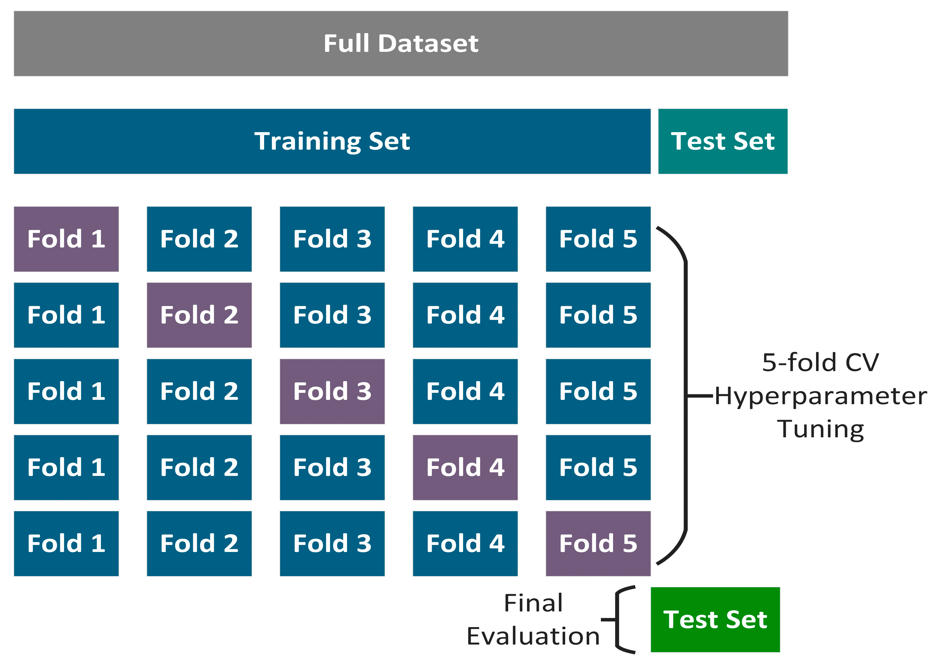
In this study, k-fold cross-validation was used to enhance model robustness. In each iteration, one subset was selected as the validation unit, and the remaining k-1 subsets were combined into the training unit. This process was repeated k times to ensure all data participated in both training and validation. For example, in 5-fold cross-validation, the dataset was divided into five equal subsets. An ensemble model was constructed through five cycles of training (Figure 1). This effectively alleviated local overfitting caused by differences in data distribution. This method can enhance the capture of nonlinear characteristics in the coupled responses between photosynthetic rate and multiple factors.

2.3.2. Algorithm Selection and Model Construction

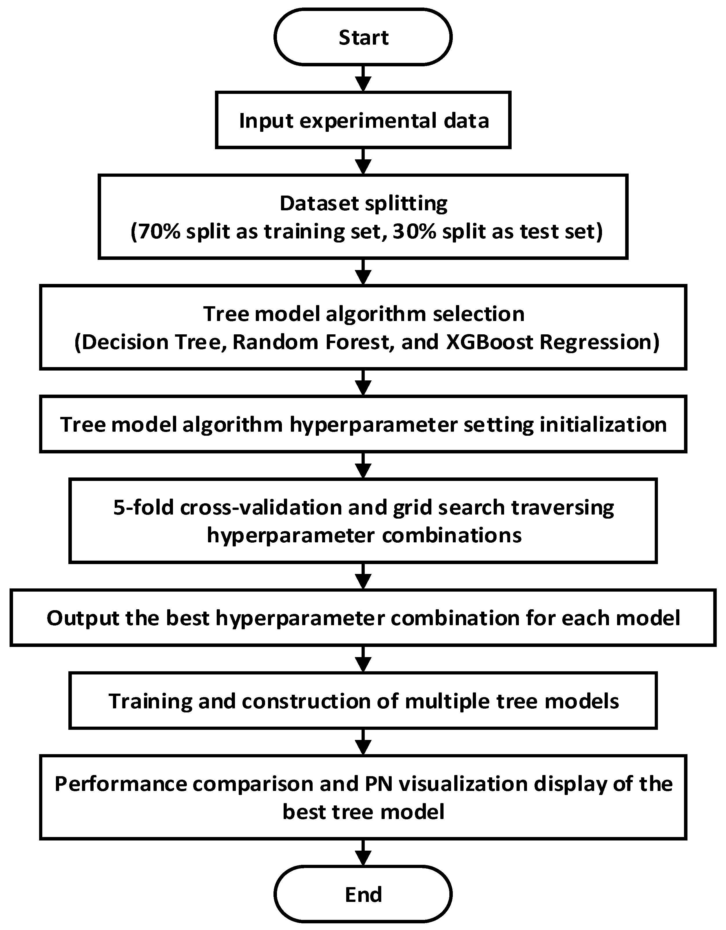
The specific workflow is illustrated in Figure 2. Firstly, the experimental data were inputted and then split into training and test sets at a 7:3 ratio. Subsequently, 5-fold cross-validation and grid search were employed to iterate through hyperparameter combinations, aiming to minimize the mean squared error (MSE) on the test set and thereby determine the optimal hyperparameter combination for each model. Finally, multiple tree models were trained. The best-performing model was then identified by comparing model performance comparison and visualizing the predicted Pn values.

DT Regression Model:

DTs are algorithms widely used in machine learning and data science, which construct decision-making models by recursively partitioning datasets into subsets [42].

Model hyperparameter selection was conducted using the GridSearchCV class within scikit-learn, which performed an exhaustive grid search across predefined hyperparameter spaces to identify the optimal configuration. The predetermined tuning ranges for the hyperparameters of the DT regression model were as follows: max_depth (maximum depth of the decision tree) in the range of 1–21, min_samples_split (minimum number of samples required to split a node) in the range of 2–6, and min_samples_leaf (minimum number of samples required at a leaf node) in the range of 1–5. All hyperparameters were tuned in integer increments of 1.

Step 1: Data Preparation

Input Data:

Feature variables were: $X \in {\mathrm{R}}^{n\times 3}$. $X_1$: (PPFD, μmol m⁻² s⁻¹), $X_2$: (CO₂ Concentration, μmol mol⁻¹), $X_3$: (Temperature, °C). The target variable was: $y \in {\mathrm{R}}^n$. Pn: (μmol m⁻² s⁻¹).

Data partitioning by Proportion: The dataset was randomly divided into a training set (70%) and a testing set (30%) via the simple random sampling method. This approach ensured both randomness and a uniform distribution of the data, thereby minimizing potential bias.

Step 2: Initialize the Root Node

Place all training data ($X_{\mathrm{train}}, y_{\mathrm{train}}$) into the root node, initially corresponding to region $R_0$.

Step 3: This study defines the recursive splitting rules for child nodes and their corresponding termination conditions, which are detailed in Equation (1).

$$\begin{array}{l}\mathrm{Tree}\left(X_{\mathrm{node}}, y_{\mathrm{node}}, D\right)=\dots \\ \left\{\begin{array}{ll}{c}_{\mathrm{node}}={\displaystyle \frac{1}{N}}{\displaystyle \sum _{i=1}^N{y}_i}\hfill & \mathrm{if} \mathrm{Termination} \mathrm{conditions} \hfill \\ 〈\left(j^{*}, s^{*}\right), \mathrm{Tree}\left(X_{\mathrm{left}}, y_{\mathrm{left}}, D+1\right), \mathrm{Tree}\left(X_{\mathrm{right}}, y_{\mathrm{right}}, D+1\right)〉\hfill & \mathrm{Otherwise}\hfill \end{array}\right.\end{array}$$

(1)

Termination Conditions:

$$\left\{\begin{array}{ll}N<N_{\mathrm{split}}\hfill & (\mathrm{when} \mathrm{the} \mathrm{node} \mathrm{has} \mathrm{insufficient} \mathrm{samples})\hfill \\ D\ge D_{\max }\hfill & (\mathrm{when} \mathrm{the} \mathrm{maximum} \mathrm{depth} \mathrm{is} \mathrm{reached})\hfill \\ \min \left(N_{\mathrm{left}}, N_{\mathrm{right}}\right)<N_{\mathrm{leaf}}\hfill & (\mathrm{when} \mathrm{the} \mathrm{child} \mathrm{node} \mathrm{has} \mathrm{insufficient} \mathrm{samples})\hfill \end{array}\right.$$

Definition of Symbols:

Data of the current node: ($X_{\mathrm{node}}, y_{\mathrm{node}}$), Sample size $N$, tree depth $D$.

Hyperparameter Specification:

$D_{\max }$ (max_depth): The maximum depth of the tree.

$N_{\mathrm{split}}$ (min_samples_split): The minimum sample size required for splitting.

$N_{\mathrm{leaf}}$ (min_samples_leaf): The minimum sample size of a leaf node.

Step 4: Splitting Criterion and Child Node Generation:

For each feature $j \in \{1, 2, 3\}$ (PPFD, CO₂, temperature) and candidate split point, calculate the weighted MSE after splitting, as shown in Equation (2).

$$\mathrm{MSE}(j,s)={\displaystyle \frac{N_{\mathrm{left}}}{N}}\cdot {\mathrm{MSE}}_{\mathrm{left}}+{\displaystyle \frac{N_{\mathrm{right}}}{N}}\cdot {\mathrm{MSE}}_{\mathrm{right}}$$

(2)

where the MSE of left child node is given by Equations (3) and (4).

$${\mathrm{MSE}}_{\mathrm{left}}={\displaystyle \frac{1}{N_{\mathrm{left}}}}{\displaystyle \sum _{i \in \mathrm{left}}{\left(y_i-c_{\mathrm{left}}\right)}^2}$$

(3)

$$c_{\mathrm{left}}={\displaystyle \frac{1}{N_{\mathrm{left}}}}{\displaystyle \sum _{i \in \mathrm{left}}{y}_i}$$

(4)

where the MSE of right child node is given by Equations (5) and (6).

$${\mathrm{MSE}}_{\mathrm{right}}={\displaystyle \frac{1}{N_{\mathrm{right}}}}{\displaystyle \sum _{i \in \mathrm{right}}{\left(y_i-c_{\mathrm{right}}\right)}^2}$$

(5)

$$c_{\mathrm{right}}={\displaystyle \frac{1}{N_{\mathrm{right}}}}{\displaystyle \sum _{i \in \mathrm{right}}{y}_i}$$

(6)

Determine the optimal split selection, as shown in Equation (7).

$$\left(j^{*}, s^{*}\right)=\arg {\min }_{j,s}\mathrm{MSE}(j, s)$$

(7)

Conduct child node partitioning, as shown in Equation (8).

$$\begin{array}{cc}{X}_{\mathrm{left}}=\left\{X_i\mid X_{i,j}\le s^{*}\right\},& y_{\mathrm{left}}=\left\{y_i\mid X_{i,j}\le s^{*}\right\}\\ X_{\mathrm{right}}=\left\{X_i\mid X_{i,j}>s^{*}\right\},& y_{\mathrm{right}}=\left\{y_i\mid X_{i,j}>s^{*}\right\}\end{array}$$

(8)

Step 5: Recursively generate subtrees, as shown in Equations (9) and (10).

Call on the left child node:

$$\mathrm{Tree}\left(X_{\mathrm{left}}, y_{\mathrm{left}}, D+1\right)$$

(9)

Call on the right child node:

$$\mathrm{Tree}\left(X_{\mathrm{right}}, y_{\mathrm{right}}, D+1\right)$$

(10)

Step 6: Generate the complete DT, as shown in Equation (11).

Once recursion terminates at Step 4, all child nodes are designated as leaf nodes, with their predicted values being the mean value of the target variable in their corresponding regions.

Final output: a complete DT structure composed of root nodes and leaf nodes, which generates the regression tree model. Here $c_m$ is the mean value of the target values of the samples within the region $R_m$.

$$T(x)=\left\{\begin{array}{ll}{c}_1\hfill & \mathrm{if} x \in R_1\hfill \\ c_2\hfill & \mathrm{if} x \in R_2\hfill \\ ⋮\hfill \\ c_m\hfill & \mathrm{if} x \in R_m\hfill \end{array}\right.$$

(11)

Step 7: DT regression model, as shown in Equation (12).

The tree regression functions are used to predict Pn for new samples, where $X_{\mathrm{new}}=(x_1, x_2, x_3)$ denotes the feature vector of the new sample.

$$y_{\mathrm{pred}}=T(X_{new})$$

(12)

Steps 1–7 detail the construction procedure of the DT regression model, which serves as the fundamental building block for subsequent ensemble models. While both RF and XGB inherit the core logic of DTs, their key differences lie in ensemble strategies and parameter optimization methods. Therefore, the implementation details of these ensemble tree models are not elaborated further herein.

RF Regression Model:

RF regression is an ensemble learning method based on DTs. It constructs multiple DTs and aggregates their predictions; during the training of each DT, random feature subset selection and bootstrap sampling are introduced to enhance model diversity and robustness [43]. This approach effectively reduces the risk of overfitting, improves prediction accuracy, and is widely applied in practical applications such as agricultural engineering environmental data modeling.

The predetermined tuning parameter ranges for the RF regression model were as follows: n_estimators in the range of 50–150; and max_depth, min_samples_split, and min_samples_leaf, with the same tuning ranges as the DT model, all with integer increments of 1.

XGB Regression Model:

XGB is an efficient ensemble learning algorithm based on Gradient Boosting Decision Trees (GBDT). It operates by sequentially constructing multiple DTs, where each subsequent tree specializes in fitting the residuals derived from the predictions of trees in the ensemble. The core optimization of XGB includes two key components: the second-order Taylor expansion of the loss function, and the integration of explicit regularization terms (L1/L2) to control model complexity. This dual optimization strategy effectively mitigates overfitting while enhancing prediction accuracy [44]. It has consistently demonstrated exceptional performance when processing structured/tabular data.

The predetermined tuning parameter ranges for the XGB regression model were as follows: learning_rate in the range of 0.1–1.0 with increments of 0.1; max_depth and n_estimators, whose tuning ranges were consistent with those of the RF model, all with integer increments of 1.

2.3.3. Model Performance Evaluation Metrics

To evaluate the performance of Pn prediction models and identify the optimal one, the following metrics were employed: root mean square error (RMSE), mean absolute error (MAE), adjusted coefficient of determination (Adjusted R²), and the Evaluation Metric Gap Ratio (EMGR)—defined as the proportional gap of evaluation metrics (e.g., RMSE, MAE, Adjusted R² Decrease) between the test and training datasets [45]. The mathematical formulas for these metrics are provided in Equations (13)–(19).

$$\mathrm{RMSE}=\sqrt{{\displaystyle \frac{1}{n}}{\displaystyle \sum _{i=1}^n{(y_i-{\widehat{y}}_i)}^2}}$$

(13)

$$\mathrm{MAE}={\displaystyle \frac{1}{n}}{\displaystyle \sum _{i=1}^n|}{y}_i-{\widehat{y}}_i|$$

(14)

$$R^2=1-{\displaystyle \frac{{\displaystyle \sum _{i=1}^n{(y_i-{\widehat{y}}_i)}^2}}{{\displaystyle \sum _{i=1}^n{(y_i-\overline{y})}^2}}}$$

(15)

$$\mathrm{Adjusted} R^2=1-{\displaystyle \frac{(1-R^2)(n-1)}{n-k-1}}$$

(16)

Evaluation Metric Gap Ratio Calculation (Test Set vs. Training Set):

$${\mathrm{RMSE}}_{\mathrm{increase}}(\%)=\left({\displaystyle \frac{{\mathrm{RMSE}}_{\mathrm{test}}}{{\mathrm{RMSE}}_{\mathrm{train}}}}-1\right)\times 100\%$$

(17)

$${\mathrm{MAE}}_{\mathrm{increase}}(\%)=\left({\displaystyle \frac{{\mathrm{MAE}}_{\mathrm{test}}}{{\mathrm{MAE}}_{\mathrm{train}}}}-1\right)\times 100\%$$

(18)

$$\mathrm{Adjusted} R^2 \mathrm{Decrease} (\%)=\left({\displaystyle \frac{R_{{\mathrm{adj}}_{\mathrm{train}}}^2-R_{{\mathrm{adj}}_{\mathrm{test}}}^2}{R_{{\mathrm{adj}}_{\mathrm{train}}}^2}}\right)\times 100\%$$

(19)

The key symbols and their definitions for model performance metrics are as follows:

$y_i$: Observed Pn for sample $i$. ${\widehat{y}}_i$: Predicted Pn for sample $i$. $\overline{y}$: Mean of observed Pn. $n$: Total number of samples in the dataset. $k$: Number of predictor variables. $i$: Sample index $(i=1,2,\cdots ,n)$.

2.3.4. Data Processing Software

In this study, the four-dimensional scatter plot illustrating the response relationship between multi-environmental driving factors (PPFD, CO₂ concentration, temperature) and Pn was generated using OriginPro 2022 (OriginLab Corporation, Northampton, MA, USA).

All modeling algorithms (DT, RF, and XGB) were implemented in a Python 3.10.16 environment (Python Software Foundation, Wilmington, DE, USA). The core algorithms were constructed using the scikit-learn library (version 1.4.2; https://scikit-learn.org/ (accessed on 15 March 2025)) and the XGBoost library (version 3.0.0; https://xgboost.ai/ (accessed on 15 March 2025)).

Model performance was evaluated based on the following metrics: RMSE, MAE, R², and Adjusted R². These metrics were calculated via functions from the sklearn.metrics module (scikit-learn library).

Post-modeling visualization diagrams for presenting model results were generated using the Matplotlib library (version 3.7.5; https://matplotlib.org/ (accessed on 15 March 2025)).

3. Results

3.1. Variation and Regulatory Mechanism Analysis of Pn Across Key Developmental Stages of Tomato in Winter Solar Greenhouses

3.1.1. Optimal Pn and Corresponding Light-Temperature-CO₂ Conditions in Tomato at Early Flowering and Fruit Development Stages Based on Experimental Data

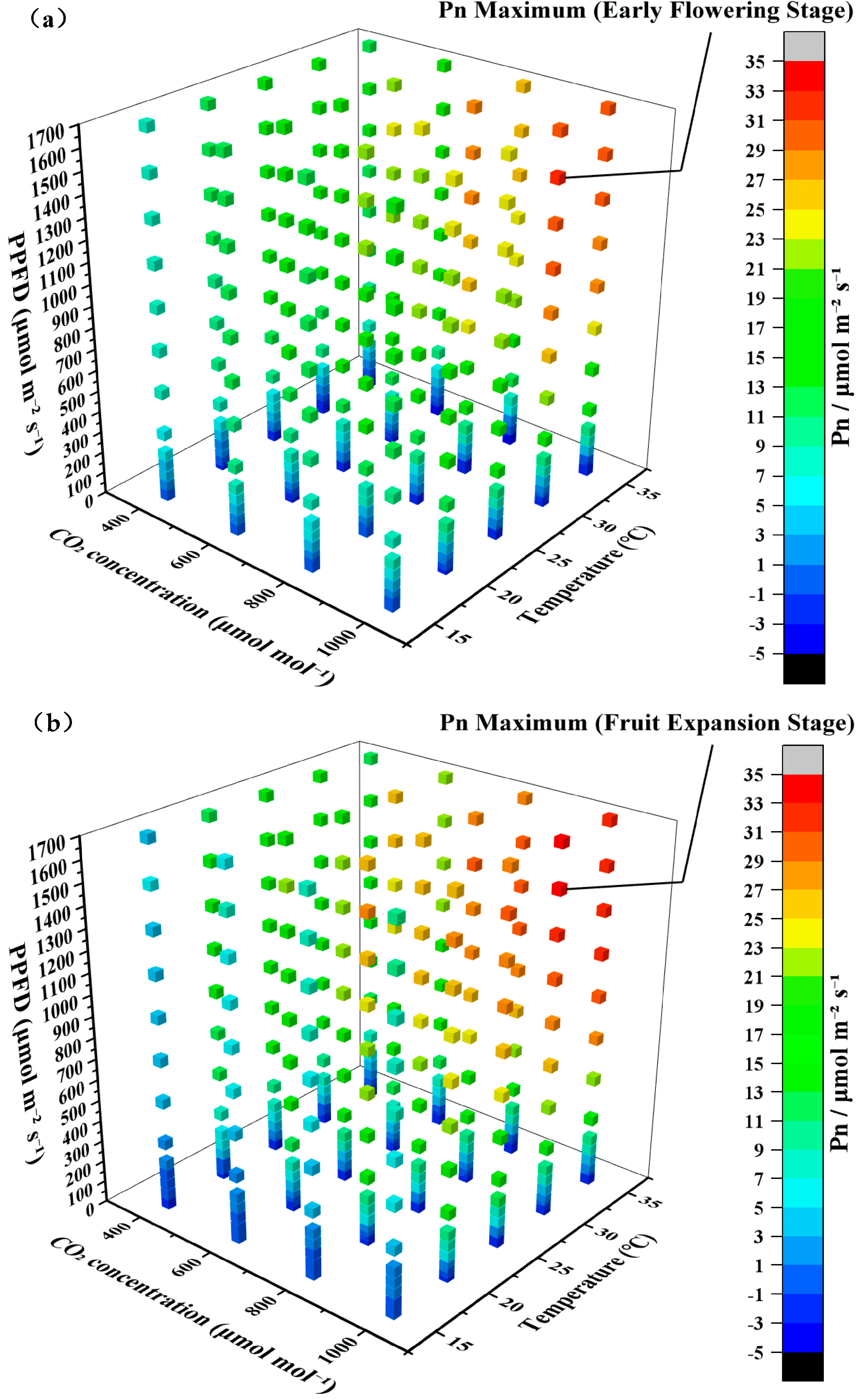
Based on Pn measurements of tomato during the early flowering and fruit development stages, the results show that both growth stages reached their respective Pn peaks (early flowering: 31.3 μmol m⁻² s⁻¹; fruit development: 34.9 μmol m⁻² s⁻¹) under the following environmental parameter combination: CO₂ concentration of 1000 μmol mol⁻¹, temperature of 30 °C, and photosynthetic photon flux density (PPFD) of 1500 μmol m⁻² s⁻¹. From the early flowering to the fruit development stage, the Pn peak increased by approximately 11.5% (Figure 3).

When temperature (30 °C) and PPFD (1500 μmol m⁻² s⁻¹) were held constant, Pn in both the early flowering and fruit development stages increased as CO₂ concentration rose from 400 to 1000 μmol mol⁻¹. Notably the fruit development stage exhibited higher sensitivity to elevated CO₂, with a faster rate of Pn increase.

Under fixed conditions of CO₂ (1000 μmol mol⁻¹) and PPFD (1500 μmol m⁻² s⁻¹), Pn of tomato leaves in both the early flowering and fruit development stages peaked at 30 °C as temperature increased from 15 °C to 35 °C. Both stages exhibited a decrease in Pn when exposed to high temperature (35 °C).

Under optimized conditions of CO₂ (1000 μmol mol⁻¹) and temperature (30 °C), the Pn of tomato leaves in both the early flowering and fruit development stages increased rapidly with rising PPFD before reaching a plateau. The fruit development stage exhibited a faster rate of Pn increase.

Based on comprehensive analysis of experimental data, the number of observation points with Pn in the high-value range (25–35 μmol m⁻² s⁻¹) was significantly higher during the fruit development stage than that during the early flowering stage. Specifically, high Pn values accounted for ~6.7% of total observations in the early flowering stage, compared to ~14.2% in the fruit development stage. For medium Pn values (11–25 μmol m⁻² s⁻¹), the proportions were ~41.7% (early flowering) and ~30.3% (fruit development), while the proportions of low Pn values (<11 μmol m⁻² s⁻¹) were ~51.4% (early flowering) and ~55.3% (fruit development), respectively.

3.1.2. Pn Trends Under the Optimal Tree-Based Model Across Tomato Developmental Stages

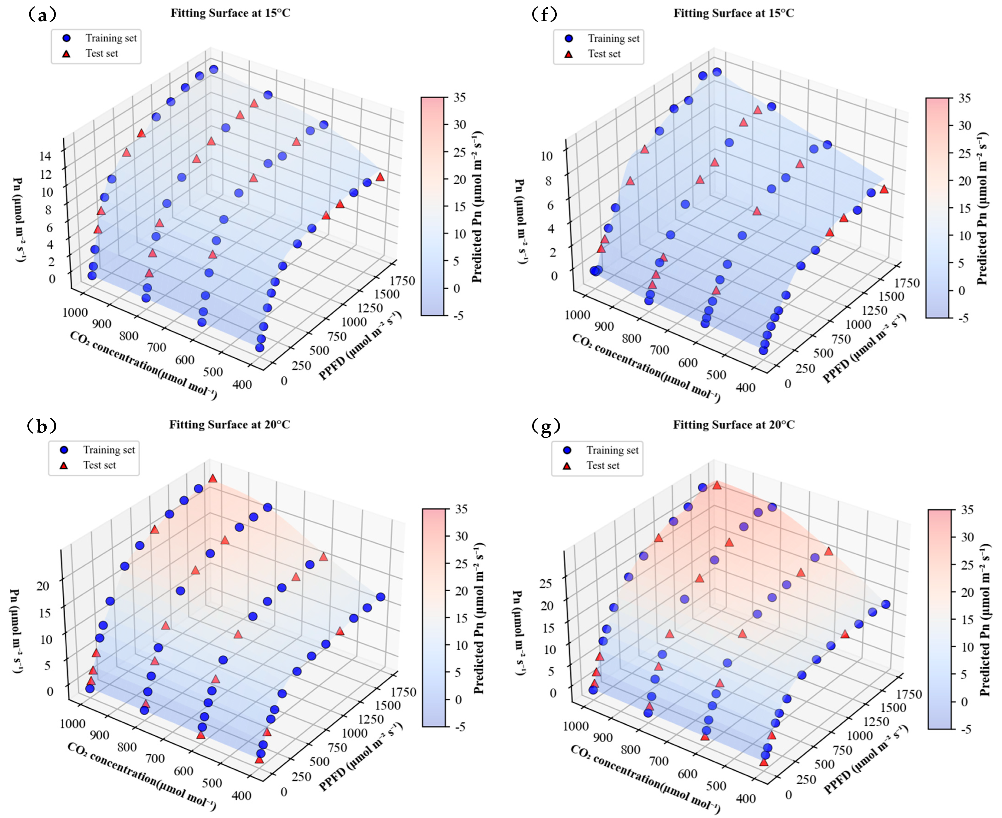
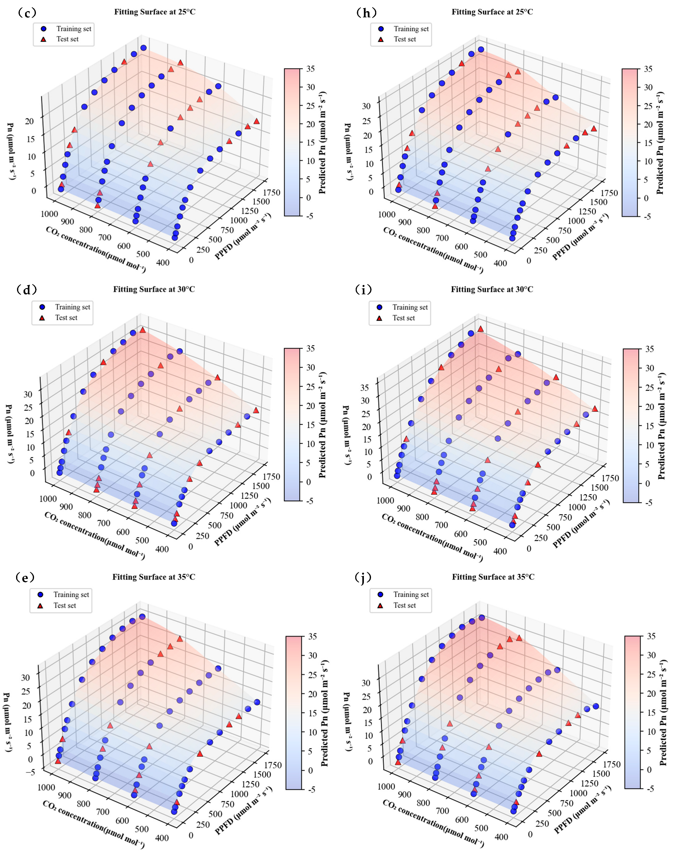
Among the tree-based models tested, the Pn prediction model constructed using the XGB algorithm exhibited the optimal fitting performance. During both the early flowering and fruit development stages, the predicted values from this model showed a high degree of consistency with experimentally measured values—consistent with the close alignment between the Pn prediction surfaces and measured data (Figure 4).

As indicated by the temperature comparisons in Figure 4, the Pn values for both critical growth stages were low at low temperatures (<20 °C) and rapidly reached saturation. Increasing temperature stimulated Pn, but this stimulatory effect shifted to inhibition when temperature exceeded 30 °C. Enhancing PPFD under specific temperature/CO₂ conditions, or elevating CO₂ concentration under constant temperature and light conditions, consistently resulted in a saturated growth pattern for Pn-characterized by an initial rapid increase followed by a gradual asymptotic leveling off.

During the fruit development stage, photosynthetic capacity was higher compared to the early flowering stage (Figure 4b–d vs. Figure 4g–i), which manifested as an upward shift of the fruit development stage’s Pn response surface in the coupled plots. However, under low-temperature (15 °C) and high-temperature (35 °C) conditions, the predicted Pn response surfaces for the fruit development stage exhibited a more significant vertical decline and a greater reduction in Pn magnitude than those for the early flowering stage (Figure 4a,e,f,j).

3.2. Prediction Results of Three Tree-Based Models for Pn in Tomato Across Key Developmental Stages

3.2.1. Evaluation of the Optimal Tree-Based Model

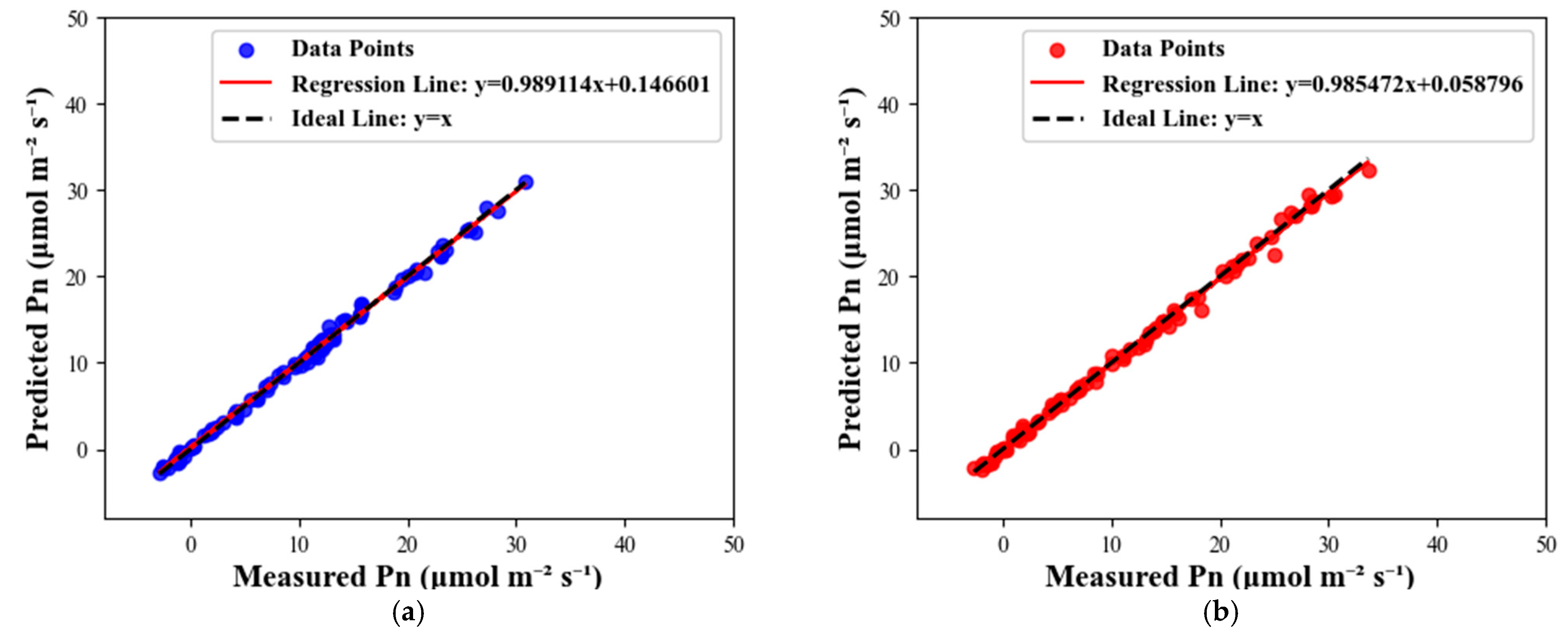
Analysis revealed that the XGB model achieved superior goodness-of-fit for tomato Pn relative to the DT and RF algorithms. As demonstrated in Figure 5, linear regressions between measured and predicted Pn values on the test set exhibited slopes approaching unity with minimal intercepts: during the early flowering stage, the regression exhibited a slope of 0.989 (intercept = 0.147; adjusted R² = 0.997). For the fruit development stage, the slope was 0.985 (intercept = 0.058; adjusted R² = 0.996). These results indicate near-ideal agreement between predicted and observed Pn values across both critical developmental stages. Comprehensive comparisons of model stability and additional performance metrics are detailed in Section 3.2.2.

3.2.2. Analysis and Prediction Results of Three Tree-Based Models

This study employed three tree-based models, namely DT, RF, and XGB, to construct Pn prediction models (

Table 1. Performance metrics of Pn prediction models for the early flowering stage across training and test datasets using DT, RF, and XGB algorithms.

Regression Algorithm	Dataset	Optimal Hyperparameters	RMSE	MAE	Adjusted R2	Overfitting Risk
DT	Training Set	max_depth: 1 min_samples_split: 4 min_samples_leaf: 1	0.4350	0.2836	0.9976	High Risk RMSE↑115% MAE↑137% R2↓1.00%
	Test Set		0.9372	0.6732	0.9876
RF	Training Set	n_estimators: 90 max_depth: 1 min_samples_split: 2 min_samples_leaf: 1	0.3011	0.2158	0.9988	High Risk RMSE↑96% MAE↑102% R2↓0.38%
	Test Set		0.5909	0.4355	0.9951
XGB	Training Set	max_depth: 3 learning_rate: 0.3 n_estimators: 110	0.2891	0.2427	0.9985	Low Risk RMSE↑62% MAE↑49% R2↓0.17%
	Test Set		0.4693	0.3616	0.9969

Note: Evaluation metrics comprise the adjusted coefficient of determination (Adjusted R²), root mean square error (RMSE, μmol m⁻² s⁻¹), and mean absolute error (MAE, μmol m⁻² s⁻¹). Overfitting risk classification requires at least 2 of the following metrics to meet the corresponding thresholds: High Risk (≥80% increase in RMSE or ≥60% increase in MAE or ≥0.25% decrease in Adjusted R²) or Low Risk (<80% increase in RMSE or <60% increase in MAE or <0.25% decrease in Adjusted R²). If the RMSE of the testing set exceeds 1.0 μmol m⁻² s⁻¹, the model is deemed to fail fundamental accuracy requirements, and the overfitting risk assessment is automatically invalidated.

and

Table 2. Performance metrics of Pn prediction models for the fruit development stage across training and test datasets using DT, RF, and XGB algorithms.

Regression Algorithm	Dataset	Optimal Hyperparameters	RMSE	MAE	Adjusted R2	Overfitting Risk
DT	Training Set	max_depth: 1 min_samples_split: 2 min_samples_leaf: 1	0.0000	0.0000	1.0000	High Risk RMSE↑∞% MAE↑∞% R2↓0.77%
	Test Set		0.8525	0.6483	0.9923
RF	Training Set	n_estimators: 110 max_depth: 9 min_samples_split: 2 min_samples_leaf: 1	0.3430	0.2488	0.9988	High Risk RMSE↑120% MAE↑134% R2↓0.49%
	Test Set		0.7550	0.5830	0.9940
XGB	Training Set	max_depth: 3 learning_rate: 0.3 n_estimators: 110	0.3457	0.2696	0.9988	Low Risk RMSE↑74% MAE↑52% R2↓0.26%
	Test Set		0.6003	0.4105	0.9962

Note: Model performance was evaluated using Adjusted R², RMSE, and MAE. Hyperparameters of all models were optimized via 5-fold cross-validation. The classification of overfitting risk (High/Low) follows the criteria defined in Table 1.

). Experimental results demonstrated that among these models, XGB consistently exhibited optimal generalization ability and prediction accuracy across the two critical phenological stages (early flowering and fruit development) of tomato in winter solar greenhouses. Specifically, XGB achieved the lowest prediction errors on the independent test set; meanwhile, it showed the smallest proportional decline in predictive performance between training and test set. Detailed performance metrics are presented as follows:

In the early flowering stage (Table 1), the XGB model exhibited exceptional predictive performance, achieving an RMSE of 0.469 μmol m⁻² s⁻¹ on the test set—50.0% lower than that of DT model (0.937 μmol m⁻² s⁻¹) and 20.7% lower than that of RF (0.591 μmol m⁻² s⁻¹). Similarly, XGB achieved the lowest MAE on the test set (0.362 μmol m⁻² s⁻¹), which was 46.2% lower than the DT model (0.673 μmol m⁻² s⁻¹) and 17.0% lower than the RF model (0.435 μmol m⁻² s⁻¹). Crucially, the XGB model was classified as having low overfitting risk, whereas DT and RF model exhibited high overfitting risk.

In the fruit development stage (Table 2), the XGB model maintained optimal predictive performance, achieving an RMSE of 0.600 μmol m⁻² s⁻¹ on the test set—this value was 29.6% lower than that of DT (0.852 μmol m⁻² s⁻¹) and 20.5% lower than that of the RF model (0.755 μmol m⁻² s⁻¹). Similarly, the MAE of the XGB model on the test set (0.411 μmol m⁻² s⁻¹) significantly outperformed the other two algorithms, with reductions of 36.6% compared to the DT model (0.648 μmol m⁻² s⁻¹) and 29.5% compared to the RF model (0.582 μmol m⁻² s⁻¹). Importantly, the XGB model retained a low overfitting risk, which stood in sharp contrast to the DT model’s catastrophic extreme overfitting and RF model’s significant accuracy degradation under high overfitting risk.

4. Discussion

Both the early flowering and fruit development stages of tomato share the same optimal conditions for maximum Pn: 1000 μmol mol⁻¹ CO₂, 30 °C, and 1500 μmol m⁻² s⁻¹ PPFD. This confirms that tomato, a typical C3 plant, retains core photosynthetic environmental requirements across key reproductive stages. This aligns with prior studies showing that 800–1000 μmol mol⁻¹ CO₂, 25–30 °C, and moderate-to-high PPFD (≥1000 μmol m⁻² s⁻¹) optimize Rubisco carboxylation efficiency and light energy conversion in tomato leaves [46,47,48]. Specifically, 1000 μmol mol⁻¹ CO₂ mitigates CO₂ limitation in closed greenhouses, while 30 °C balances photosynthetic and respiratory enzyme activity—avoiding metabolic slowdown at low temperatures and damage at high temperatures [49,50].

The fruit development stage exhibits an 11.5% higher Pn peak (34.9 μmol m⁻² s⁻¹) than the early flowering stage (31.3 μmol m⁻² s⁻¹). This result is consistent with the previous data on the photosynthetic performance of the entire canopy of tomatoes at different growth stages [51]. This reflects dynamic shifts in source-sink relationships during tomato development. It supports the classic source-sink theory, where stronger sink strength (from developing fruits) boosts source activity (leaf photosynthesis) [52]. Developing fruits act as strong metabolic sinks, stimulating the transport of photosynthetic assimilates via hormonal signals (e.g., cytokinins) and upregulating key enzymes like cell wall invertase [52]. This regulation not only increases maximum photosynthetic capacity but also improves carbon partitioning efficiency—consistent with 14–47% yield gains in tomato through source-sink optimization [52]. Pn value distributions further confirm stage-specific photosynthetic capacity: 14.2% of observations fall in the high range (25–35 μmol m⁻² s⁻¹) during fruit development, compared to 6.7% in early flowering. The higher share of high Pn values in fruit development directly ties to stronger sink demand. Meanwhile, the slightly higher proportion of low Pn values (~55.3%) may indicate greater sensitivity to microenvironmental fluctuations (e.g., transient light limitation or temperature spikes) [46,53]. This underscores the need for precise environmental control during fruit development to sustain high photosynthetic efficiency.

The fruit development stage showed greater sensitivity to elevated CO₂, with faster Pn increases as CO₂ rose from 400 to 1000 μmol mol⁻¹. This highlights stage-specific physiological adjustments. It aligns with findings that C3 plants in sink-dominant stages respond more strongly to CO₂ enrichment. Increased carboxylation efficiency here directly supports assimilate allocation to growing sinks [54]. In contrast, the early flowering stage—focused on initiating reproductive organs—may prioritize resource allocation to floral development over photosynthetic machinery, leading to a weaker CO₂ response [55,56]. Under optimized CO₂ and temperature, Pn rose rapidly with increasing PPFD before plateauing in both stages, with faster growth in fruit development. This points to enhanced light utilization efficiency during fruit development. It may link to upregulated electron transport in Photosystem II (PSII) and increased chlorophyll content—adaptations that support higher ATP and NADPH production for carbon fixation. The earlier plateau in fruit development further suggests coordination between light capture and CO₂ utilization. This ensures efficient conversion of light energy into assimilates under sink demand [54].

In summary, tomato maintains consistent optimal light-temperature-CO₂ conditions for Pn across early flowering and fruit development, but stage-specific photosynthetic responses are shaped by shifting source-sink relationships. These findings provide a basis for precision greenhouse management.

Owing to constraints in research resources and experimental conditions, this study only compared two critical growth stages of tomato plants, namely the early flowering stage and the fruit development stage. However, the photosynthetic physiological traits of tomatoes grown in winter solar greenhouses undergo continuous changes throughout their entire growth cycle. Focusing solely on these two stages may fail to fully capture the dynamic evolution of photosynthetic responses during the transition from vegetative growth to reproductive growth. In future research, additional sampling should be conducted across growth stages (e.g., seedling stage, peak flowering and fruit-setting stage, color-turning stage) to enable more continuous monitoring. This approach will facilitate the establishment of a dynamic prediction model that covers the entire growth cycle of tomato plants.

The sustained advantage of XGB in predicting Pn stems from its gradient boosting framework. Compared to a single DT model, XGB sequentially constructs multiple weak learners (i.e., shallow DTs) and continuously corrects the residuals of preceding models, which significantly enhances the model’s prediction accuracy and generalization capability [57]. Although individual DTs offer high interpretability, they are highly susceptible to overfitting when processing high-dimensional, complex photosynthetic data with strong nonlinear relationships—this issue drastically diminishes their predictive performance on unseen data. When compared to RF, another tree-based method, the core strength of XGB lies in its sequential optimization strategy. RF independently builds a set of decision trees and aggregates their predictions through feature subset sampling (mtry) and bootstrap sampling (bagging), which effectively improves model robustness and mitigates overfitting. However, unlike boosting algorithms, the individual trees in RF are constructed independently and lack the ability to perform sequentially optimization or assign increasing weights to focus on misclassified samples [40]. Building on the foundation of gradient boosting, XGB incorporates several key innovations: first, it leverages the second-order derivatives of the loss function (MSE) to achieve more accurate gradient direction optimization and tree structure evaluation; second, it explicitly integrates regularization terms (L1 and L2 regulation) into the objective function to penalize excessive model complexity (e.g., the weights of leaf nodes and the overall tree structure). This provides a regulation mechanism that is both distinct from RF and highly controllable [41]. Consequently, XGB typically exhibits higher prediction accuracy than RF when applied to independent test sets.

Certain comparisons of specific physiological parameters between stages were excluded because the study’s primary goal was to identify optimal environmental combinations for each stage, rather than describing inherent physiological differences between them. The findings of this study can effectively contribute to the development of precision environmental control systems for tomato production in solar greenhouses. By integrating the XGB prediction model with real-time dynamic monitoring of core environmental parameters inside the facility (e.g., PPFD, CO₂ concentration, temperature), the Pn during the early flowering and fruit development stages can be rapidly and accurately estimated. This enables the formulation of stage-specific environmental optimization strategies. Beyond providing an actionable decision-making basis for the on-demand precise regulation of solar greenhouse microclimates—thereby synergistically enhancing tomato yield and quality—this multi-dimensional modeling framework, which incorporates growth stage-specific characteristics, also offers a technical methodology for achieving efficient photosynthetic production in other crops under similar controlled environments. Notably, the model can potentially be extended to a dynamic whole-growth-cycle prediction tool, encompassing key stages such as the seedling stage, full-bloom stage, and fruit color-turning stage, further highlighting its broad application prospects.

5. Conclusions

This study revealed differential changes in the photosynthetic physiological responses of winter-grown solar greenhouse tomatoes across two key growth stages: the early flowering stage and the fruit development stage. Compared to the early flowering stage, the fruit development stage exhibited higher photosynthetic potential. However, it also displayed increased sensitivity to fluctuations in light, temperature, CO₂, and other environmental factors—necessitating more stringent, high-precision environmental control strategies. The XGB model was employed in this research, and its nonlinear analytical capability enabled the precise quantification of the complex interactions among light-temperature-CO₂ factors and their impacts on photosynthesis. The predictive accuracy of the XGB model outperformed that of conventional tree-based algorithms (DT and RF). As such, this model provides a critical quantitative tool for achieving precise environmental control in protected cultivation. This work advances the understanding of photosynthetic adaptability in solar greenhouse-grown tomatoes, with particular emphasis on elucidating the differential responses to environmental changes across distinct growth stages. Furthermore, the established XGB model serves as a key quantitative tool for developing high-precision, coordinated light-temperature-CO₂ control strategies tailored to the elevated accuracy requirements of solar greenhouse operations.

References

1. Naseer, M.; Persson, T.; Righini, I.; Stanghellini, C.; Maessen, H.; Verheul, M.J. Bio-economic evaluation of greenhouse designs for seasonal tomato production in Norway. Biosyst. Eng. 2021, 212, 413–430. [Google Scholar] [CrossRef]
2. Gatahi, D.M. Challenges and opportunities in tomato production chain and sustainable standards. Int. J. Hortic. Sci. Technol. 2020, 7, 235–262. [Google Scholar] [CrossRef]
3. Cammarano, D.; Jamshidi, S.; Hoogenboom, G.; Ruane, A.C.; Niyogi, D.; Ronga, D. Processing tomato production is expected to decrease by 2050 due to the projected increase in temperature. Nat. Food 2022, 3, 437–444. [Google Scholar] [CrossRef]
4. Imran. Growing of off-season tomato in high tunnel and its nutritional value augmentation with integrated nutrients management. J. Plant Nutr. 2023, 46, 1009–1018. [Google Scholar] [CrossRef]
5. Cui, X.; Guan, Z.; Morgan, K.; Huang, K.-M.; Hammami, A. Multitiered fresh produce supply chain: The case of tomatoes. Horticulturae 2022, 8, 1204. [Google Scholar] [CrossRef]
6. Capobianco-Uriarte, M.D.L.M.; Aparicio, J.; De Pablo-Valenciano, J.; Casado-Belmonte, M.D.P. The European tomato market. An approach by export competitiveness maps. PLoS ONE 2021, 16, e0250867. [Google Scholar] [CrossRef] [PubMed]
7. Lopes Sobrinho, O.P.; Dos Santos, L.N.S.; Soares, F.A.L.; Teixeira, M.B.; Reis, M.N.O.; Bessa, L.A.; Vitorino, L.C. Adjusting irrigation and phosphate fertilizer to optimize tomato growth and production. Agronomy 2024, 14, 1616. [Google Scholar] [CrossRef]
8. Sagar, A.; Singh, P.K. Economic feasibility of tomato (Solanum lycopersicum) production under protected and unprotected environment. Indian J. Agric. Sci. 2023, 93, 523–528. [Google Scholar] [CrossRef]
9. Banjare, C.; Mahanta, D.; Sahu, P.; Choudhary, R. A comprehensive review on protected cultivation: Importance, scope and status. Int. J. Environ. Clim. Change 2024, 14, 46–55. [Google Scholar] [CrossRef]
10. Banoo, A.; Hussain, S.; Hussain, N.; Hussain, A.; Khan, F.A.S.; Dar, S.R. Tomato performance in a protected structure: A review. Adv. Res. 2024, 25, 29–37. [Google Scholar] [CrossRef]
11. Mainar-Toledo, M.D.; González García, I.; Leiva, H.; Fraser, J.; Persson, D.; Parker, T. Environmental and economic benefits of waste heat recovery as a symbiotic scenario in sweden. Energies 2025, 18, 1636. [Google Scholar] [CrossRef]
12. Titov, A.F.; Shibaeva, T.G.; Ikkonen, E.N.; Sherudilo, E.G. Plant responses to a daily short-term temperature drop: Phenomenology and mechanisms. Russ. J. Plant Physiol. 2020, 67, 1003–1017. [Google Scholar] [CrossRef]
13. Aguilar-Rodriguez, C.E.; Flores-Velazquez, J.; Ojeda-Bustamante, W.; Rojano, F.; Iñiguez-Covarrubias, M. Valuation of the energy performance of a greenhouse with an electric heater using numerical simulations. Processes 2020, 8, 600. [Google Scholar] [CrossRef]
14. Palmitessa, O.D.; Pantaleo, M.A.; Santamaria, P. Applications and development of LEDs as supplementary lighting for tomato at different latitudes. Agronomy 2021, 11, 835. [Google Scholar] [CrossRef]
15. Li, Y.; Hoch, G. The sensitivity of root water uptake to cold root temperature follows species-specific upper elevational distribution limits of temperate tree species. Plant Cell Environ. 2024, 47, 2192–2205. [Google Scholar] [CrossRef] [PubMed]
16. Aluko, O.O.; Li, C.; Wang, Q.; Liu, H. Sucrose utilization for improved crop yields: A review article. J. Mol. Sci. 2021, 22, 4704. [Google Scholar] [CrossRef] [PubMed]
17. Guo, B.; Zhou, B.; Zhang, Z.; Li, K.; Wang, J.; Chen, J.; Papadakis, G. A critical review of the status of current greenhouse technology in China and development prospects. Appl. Sci. 2024, 14, 5952. [Google Scholar] [CrossRef]
18. Bunce, J. Changes in the responses of leaf gas exchange to temperature and photosynthesis model parameters in four C3 species in the field. Plants 2025, 14, 550. [Google Scholar] [CrossRef]
19. Petruccelli, R.; Bartolini, G.; Ganino, T.; Zelasco, S.; Lombardo, L.; Perri, E.; Durante, M.; Bernardi, R. Cold stress, freezing adaptation, varietal susceptibility of Olea europaea L.: A review. Plants 2022, 11, 1367. [Google Scholar] [CrossRef]
20. Li, Y.; Xu, W.; Ren, B.; Zhao, B.; Zhang, J.; Liu, P.; Zhang, Z. High temperature reduces photosynthesis in maize leaves by damaging chloroplast ultrastructure and photosystem II. J. Agron. Crop Sci. 2020, 206, 548–564. [Google Scholar] [CrossRef]
21. Ahmed, H.A.; Tong, Y.; Li, L.; Sahari, S.Q.; Almogahed, A.M.; Cheng, R. Integrative effects of CO2 concentration, illumination intensity and air speed on the growth, gas exchange and light use efficiency of lettuce plants grown under artificial lighting. Horticulturae 2022, 8, 270. [Google Scholar] [CrossRef]
22. Esmaili, M.; Aliniaeifard, S.; Mashal, M.; Ghorbanzadeh, P.; Seif, M.; Gavilan, M.U.; Carrillo, F.F.; Lastochkina, O.; Li, T. CO2 enrichment and increasing light intensity till a threshold level, enhance growth and water use efficiency of lettuce plants in controlled environment. Not. Bot. Horti Agrobot. Cluj-Napoca 2020, 48, 2244–2262. [Google Scholar] [CrossRef]
23. Drag, D.W.; Slattery, R.; Siebers, M.; DeLucia, E.H.; Ort, D.R.; Bernacchi, C.J. Soybean photosynthetic and biomass responses to carbon dioxide concentrations ranging from pre-industrial to the distant future. J. Exp. Bot. 2020, 71, 3690–3700. [Google Scholar] [CrossRef] [PubMed]
24. Zhang, F.; Jiang, N.; Zhang, H.; Huo, Z.; Yang, Z. Effect of low temperature on photosynthetic characteristics, senescence characteristics, and endogenous hormones of winter wheat “ji mai 22” during the jointing stage. Agronomy 2023, 13, 2650. [Google Scholar] [CrossRef]
25. Yang, J.; Qiao, H.; Wu, C.; Huang, H.; Nzambimana, C.; Jiang, C.; Wang, J.; Tang, D.; Zhong, W.; Du, K.; et al. Physiological and transcriptome responses of sweet potato [Ipomoea batatas (L.) lam] to weak-light stress. Plants 2024, 13, 2214. [Google Scholar] [CrossRef]
26. Ye, Z.; Yang, X.; Ye, Z.; An, T.; Duan, S.; Kang, H.; Wang, F. Evaluating photosynthetic models and their potency in assessing plant responses to changing oxygen concentrations: A comparative analysis of An–Ca and An–Ci curves in Lolium perenne and Triticum aestivum. Front. Plant Sci. 2025, 16, 1575217. [Google Scholar] [CrossRef]
27. Guo, Y.; Lv, Y. Evaluation of models for describing photosynthetic light–response curves and estimating parameters in rice leaves at various canopy positions. Agronomy 2025, 15, 125. [Google Scholar] [CrossRef]
28. Hu, H.; Jiang, W.; Fan, X. Estimating CO2 response in a mixed broadleaf forest using the dynamic assimilation technique. BMC Plant Biol. 2025, 25, 79. [Google Scholar] [CrossRef]
29. Li, J.; Zhu, D.; Li, C. Comparative analysis of BPNN, SVR, LSTM, Random Forest, and LSTM-SVR for conditional simulation of non-Gaussian measured fluctuating wind pressures. Mech. Syst. Signal Process. 2022, 178, 109285. [Google Scholar] [CrossRef]
30. Endo, T. Analysis of conventional feature learning algorithms and advanced deep learning models. J. Robot. Spectr. 2023, 1, 1–12. [Google Scholar] [CrossRef]
31. Lu, Z.; Yao, W.; Pei, S.; Lu, Y.; Liang, H.; Xu, D.; Li, H.; Yu, L.; Zhou, Y.; Liu, Q. Inversion of soybean net photosynthetic rate based on UAV multi-source remote sensing and machine learning. Agronomy 2024, 14, 1493. [Google Scholar] [CrossRef]
32. Zhang, X.; Huang, Z.; Su, X.; Siu, A.; Song, Y.; Zhang, D.; Fang, Q. Machine learning models for net photosynthetic rate prediction using poplar leaf phenotype data. PLoS ONE 2020, 15, e0228645. [Google Scholar] [CrossRef]
33. Ojo, M.O.; Zahid, A. Deep learning in controlled environment agriculture: A review of recent advancements, challenges and prospects. Sensors 2022, 22, 7965. [Google Scholar] [CrossRef]
34. Zhang, P.; Zhang, Z.; Li, B.; Zhang, H.; Hu, J.; Zhao, J. Photosynthetic rate prediction model of newborn leaves verified by core fluorescence parameters. Sci. Rep. 2020, 10, 3013. [Google Scholar] [CrossRef]
35. Tao, T.; Wei, X. A hybrid CNN–SVM classifier for weed recognition in winter rape field. Plant Methods 2022, 18, 29. [Google Scholar] [CrossRef]
36. Tong, Z.; Zhang, S.; Yu, J.; Zhang, X.; Wang, B.; Zheng, W. A hybrid prediction model for CatBoost tomato transpiration rate based on feature extraction. Agronomy 2023, 13, 2371. [Google Scholar] [CrossRef]
37. Engler, N.; Krarti, M. Review of energy efficiency in controlled environment agriculture. Renew. Sustain. Energy Rev. 2021, 141, 110786. [Google Scholar] [CrossRef]
38. Zamski, E.; Schaffer, A.A. Photoassimilate Distribution Plants and Crops Source-Sink Relationships, 3rd ed.; CRC: New York, NY, USA, 1996; pp. 709–724. [Google Scholar]
39. Fan, Z.; You, Z. Research on network intrusion detection based on XGBoost algorithm and multiple machine learning algorithms. Theor. Nat. Sci. 2024, 31, 161–166. [Google Scholar] [CrossRef]
40. Wang, T. Research on machine learning-based forecasting models for SSE indexes-analysis from the perspective of quantitative time-timing. Trans. Comput. Sci. Intell. Syst. Res. 2024, 5, 1774–1785. [Google Scholar] [CrossRef]
41. Deshmukh, M.; Jaiswar, A.; Joshi, O.; Shedge, R. Farming assistance for soil fertility improvement and crop prediction using XGBoost. ITM Web Conf. 2022, 44, 03022. [Google Scholar] [CrossRef]
42. Blockeel, H.; Devos, L.; Frénay, B.; Nanfack, G.; Nijssen, S. Decision trees: From efficient prediction to responsible AI. Front. Artif. Intell. 2023, 6, 1124553. [Google Scholar] [CrossRef] [PubMed]
43. Biau, G.; Scornet, E. A random forest guided tour. TEST 2016, 25, 197–227. [Google Scholar] [CrossRef]
44. Ser, G.; Bati, C.T. Modelling overdispersed seed germination data: Xgboost’s performance. J. Anim. Plant Sci. 2023, 33, 744–752. [Google Scholar] [CrossRef]
45. Chicco, D.; Warrens, M.J.; Jurman, G. The coefficient of determination R-squared is more informative than SMAPE, MAE, MAPE, MSE and RMSE in regression analysis evaluation. PeerJ Comput. Sci. 2021, 7, e623. [Google Scholar] [CrossRef]
46. Mortensen, L.M. CO2 enrichment in greenhouses. Crop responses. Sci. Hortic. 1987, 33, 1–25. [Google Scholar] [CrossRef]
47. Li, T.; Ji, Y.; Zhang, M.; Sha, S.; Li, M. Universality of an improved photosynthesis prediction model based on PSO-SVM at all growth stages of tomato. Int. J. Agric. Biol. Eng. 2017, 10, 63–73. [Google Scholar] [CrossRef]
48. Kläring, H.P.; Krumbein, A. The effect of constraining the intensity of solar radiation on the photosynthesis, growth, yield and product quality of tomato. J. Agron. Crop Sci. 2013, 199, 351–359. [Google Scholar] [CrossRef]
49. Atkin, O.K.; Tjoelker, M.G. Thermal acclimation and the dynamic response of plant respiration to temperature. Trends Pant Sci. 2003, 8, 343–351. [Google Scholar] [CrossRef]
50. Rangaswamy, T.C.; Sridhara, S.; Manoj, K.N.; Gopakkali, P.; Ramesh, N.; Shokralla, S.; Zin El-Abedin, T.K.; Almutairi, K.F.; Elansary, H.O. Impact of elevated CO2 and temperature on growth, development and nutrient uptake of tomato. Horticulturae 2021, 7, 509. [Google Scholar] [CrossRef]
51. McAvoy, R.J.; Janes, H.W. Tomato plant photosynthetic activity as related to canopy age and tomato development. J. Am. Soc. Hortic. Sci. 1989, 114, 478–482. [Google Scholar] [CrossRef]
52. Lou, H.; Li, S.; Shi, Z.; Yang, Y.; Li, Z.; Xu, C. Engineering source-sink relations by prime editing confers heat-stress resilience in tomato and rice. Cell 2025, 188, 530–549. [Google Scholar] [CrossRef] [PubMed]
53. Aslani, L.; Gholami, M.; Mobli, M.; Sabzalian, M.R. The influence of altered sink-source balance on the plant growth and yield of greenhouse tomato. Physiol. Mol. Biol. Plants 2020, 26, 2109–2123. [Google Scholar] [CrossRef]
54. Shin, J.; Hwang, I.; Kim, D.; Kim, J.; Kim, J.H.; Son, J.E. Waning advantages of CO2 enrichment on photosynthesis and productivity due to accelerated phase transition and source-sink imbalance in sweet pepper. Sci. Hortic. 2022, 301, 111130. [Google Scholar] [CrossRef]
55. Aboelyazeed, D.; Xu, C.; Hoffman, F.M.; Liu, J.; Jones, A.W.; Rackauckas, C.; Lawson, K.; Shen, C. A differentiable, physics-Informed ecosystem modeling and learning framework for large-scale inverse problems: Demonstration with photosynthesis simulations. Biogeosciences 2023, 20, 2671–2692. [Google Scholar] [CrossRef]
56. Qian, T.; Dieleman, J.A.; Elings, A.; Marcelis, L.F.M. Leaf photosynthetic and morphological responses to elevated CO2 concentration and altered fruit number in the semi-closed greenhouse. Sci. Hortic. 2012, 145, 1–9. [Google Scholar] [CrossRef]
57. Jin, Y. Optimization of XGBoost bankruptcy prediction based on four-vector optimization algorithm. Appl. Comput. Eng. 2024, 120, 42–49. [Google Scholar] [CrossRef]
Figure 1. Topology diagram of the k-fold cross-validation.
Horticulturae 11 01367 g001
Figure 2. Machine learning workflow for regression using tree-based algorithms.
Horticulturae 11 01367 g002
Figure 3. Unified-color-scale analysis of Pn in tomato leaves across developmental stages: (a) early flowering stage and (b) fruit development stage. This analysis shows the responses of Pn to temperature, CO2 concentration, and PPFD, using an identical color gradient (−5 to 35 μmol m−2 s−1; blue = minimum, red = maximum) designed to enable direct comparison of Pn distribution patterns and environmental sensitivity. Both stages reached their maximum Pn values (early flowering stage: 31.3 μmol m−2 s−1; fruit development stage: 34.9 μmol m−2 s−1) under the conditions of 30 °C, 1000 μmol mol−1 CO2, and 1500 μmol m−2 s−1 PPFD, while the fruit development stage exhibited more rapid Pn variations under synergistic environmental regulation.
Horticulturae 11 01367 g003
Figure 4. Comparison of predicted Pn (3D surfaces) from the XGB model with measured Pn values (training set: blue circles; testing set: orange triangles) under different temperature conditions. (ae) Early flowering stage: (a) 15 °C, (b) 20 °C, (c) 25 °C, (d) 30 °C, (e) 35 °C. (fj) Fruit expansion stage: (f) 15 °C, (g) 20 °C, (h) 25 °C, (i) 30 °C, (j) 35 °C. The color gradient represents predicted Pn values ranging from −5 to 35 μmol m−2 s−1. The coupled response surfaces reveal the highly nonlinear adaptive characteristics of plant photosynthesis to combined environmental factors.
Horticulturae 11 01367 g004aHorticulturae 11 01367 g004b
Figure 5. Comparison of predicted versus measured Pn values on the test set for the XGB algorithm across different tomato developmental stages. (a) Early flowering stage. (b) Fruit development stage. The black dashed line denotes the 1:1 ideal relationship; red solid lines represent linear regression fitting lines.
Horticulturae 11 01367 g005