
Predicting Sweet Pepper Yield Based on Fruit Counts at Multiple Ripeness Stages Monitored by an AI-Based System Mounted on a Pipe-Rail Trolley †

 , , , and
Abstract
1. Introduction
2. Materials and Methods
2.1. Plant Materials and Greenhouse Specifications
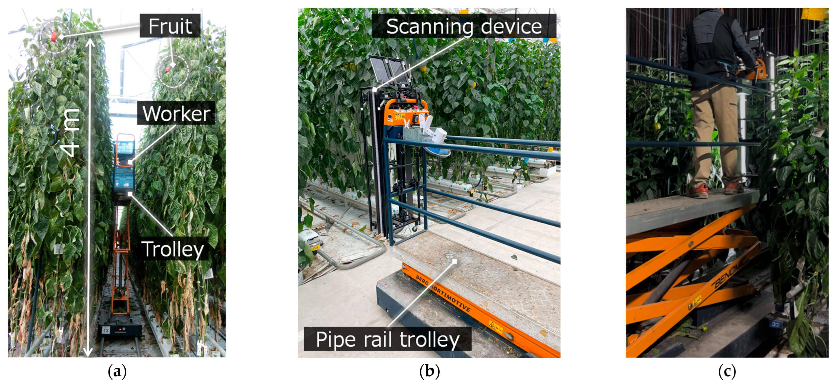
2.2. Sweet Pepper Fruit Monitoring System
2.2.1. Fruit-Scanning Device with Dual Cameras
2.2.2. Automatic Data Transfer and Analysis Process
2.2.3. Fruit Detection Model
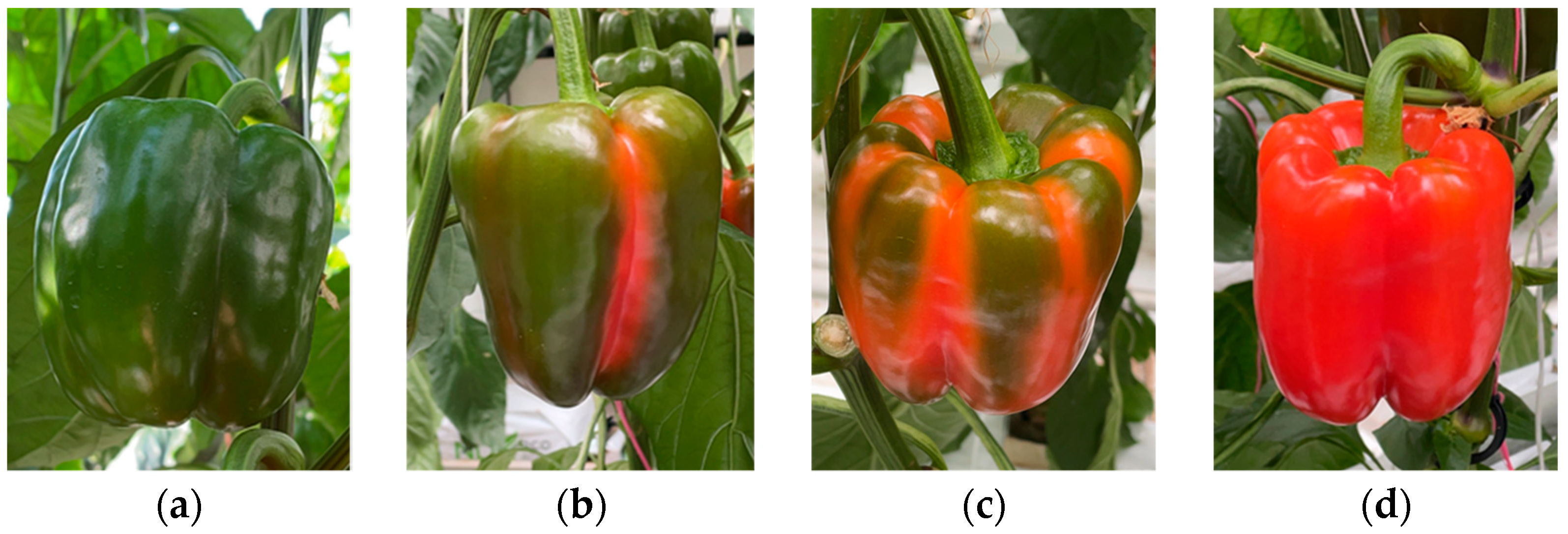
2.2.4. Fruit Maturity Classification
- 0%: Enlargement stage;
- 1–40%: Early maturation stage;
- 41–80%: Mid-to-late maturation stage;
- 81–100%: Ripe fruit.
2.3. On-Site Trials of Continuous Fruit Monitoring in a Commercial Sweet Pepper Greenhouse
2.3.1. Fruit Detection Performance
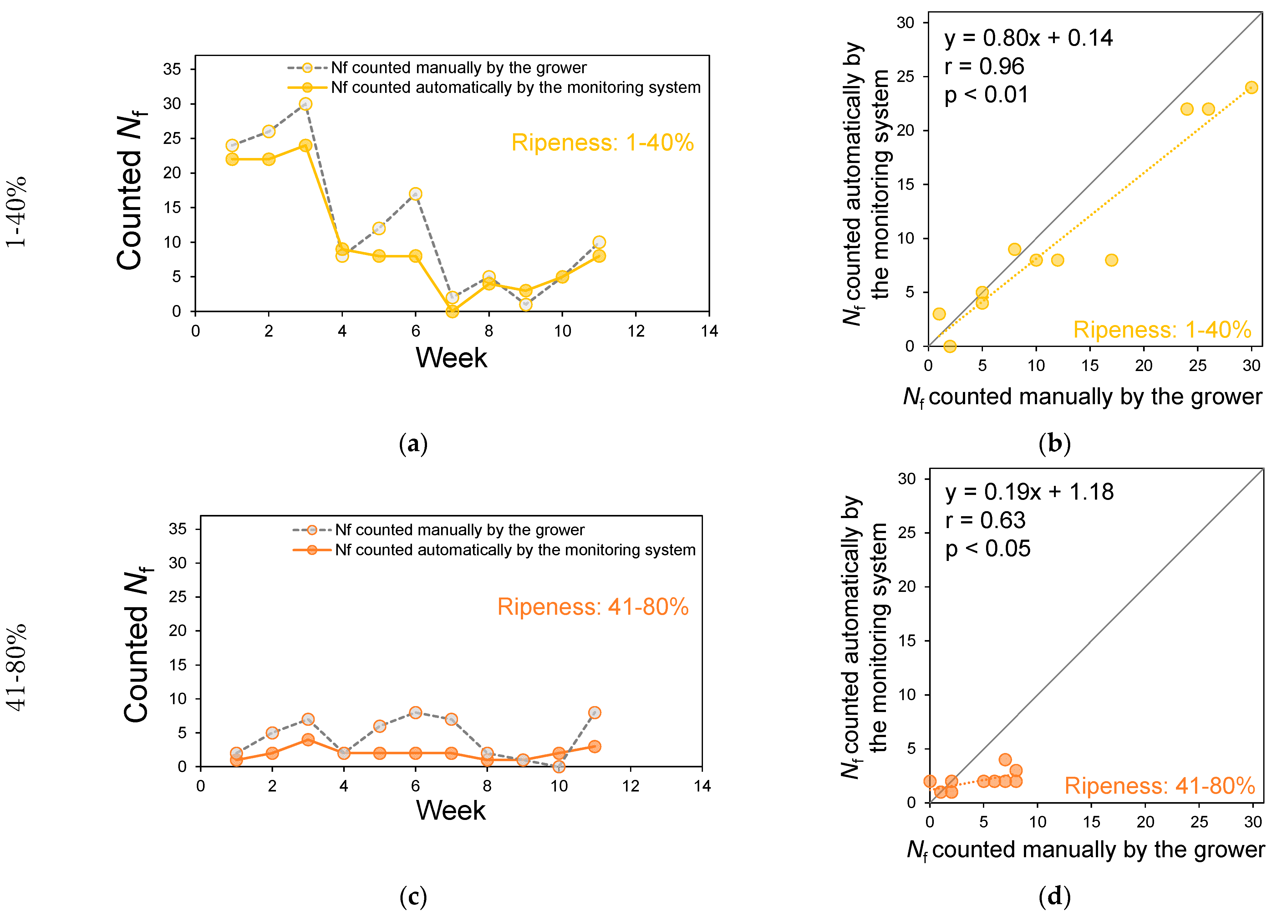
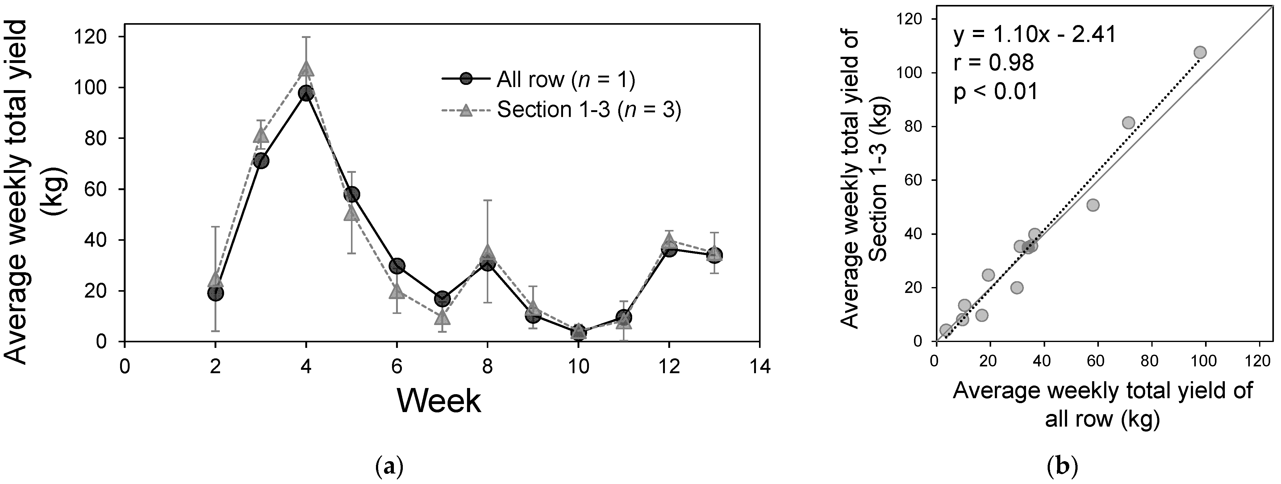
2.3.2. Counting Performance for Colored Sweet Pepper Fruits
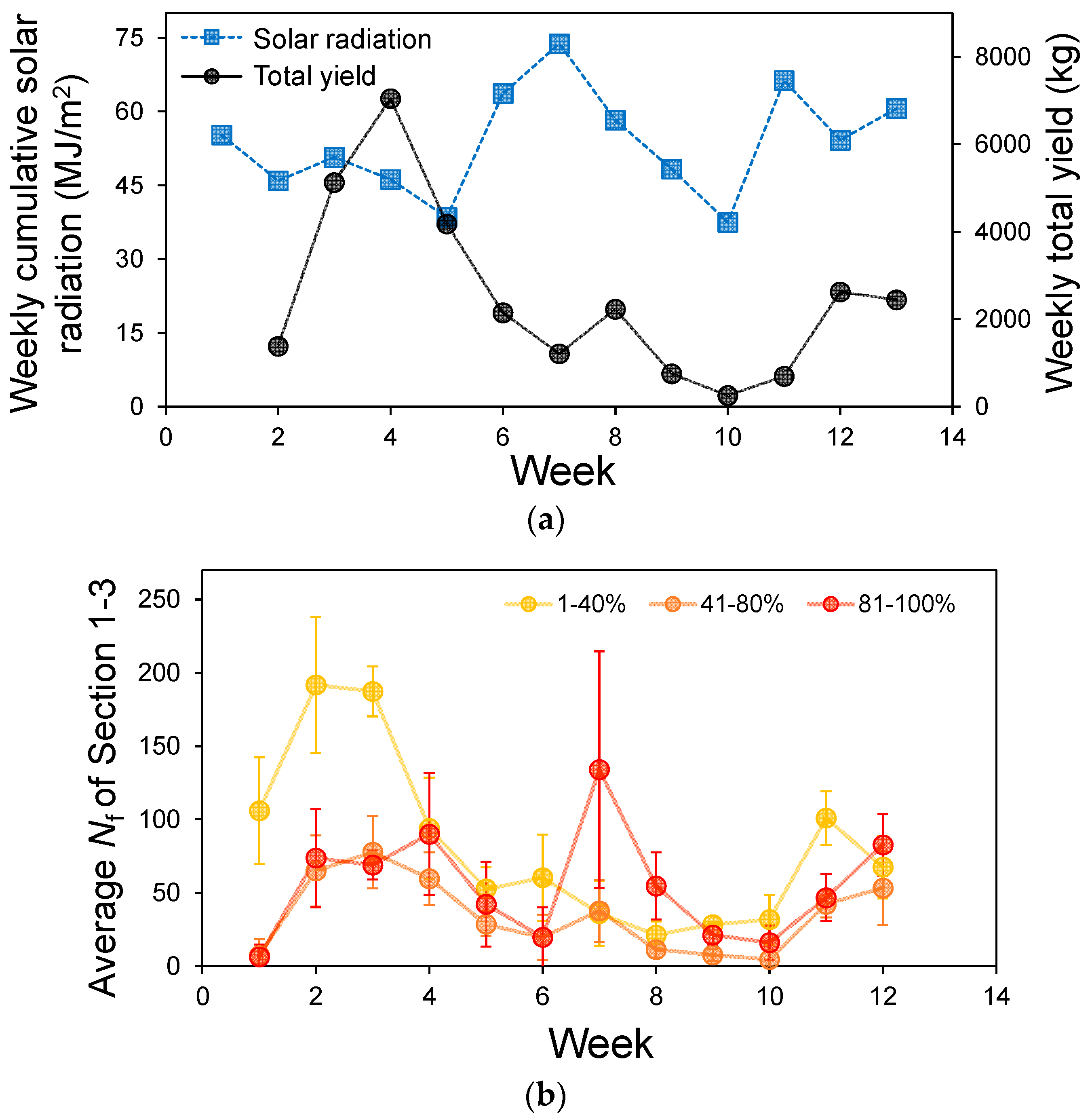
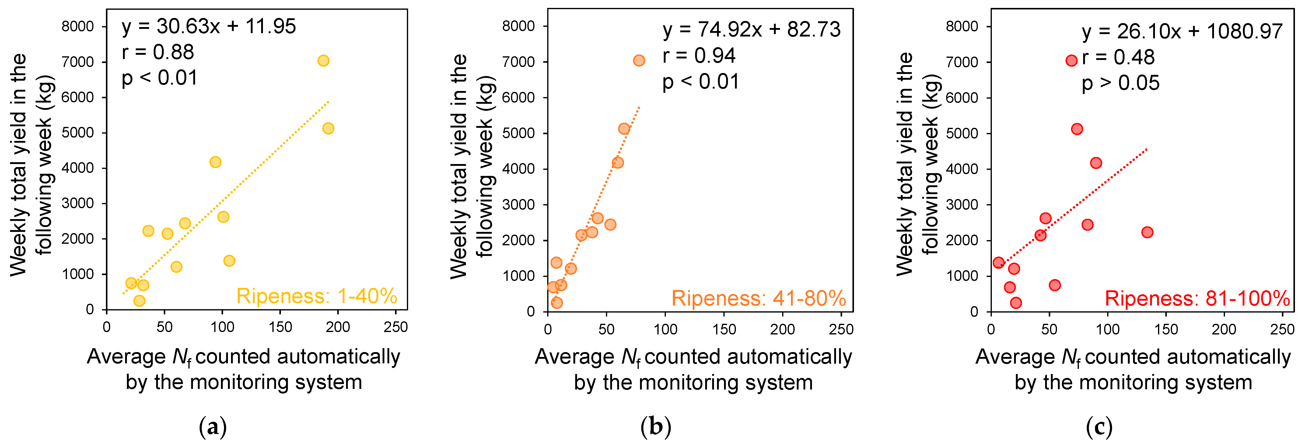
2.3.3. Relationship Between the Number of Detected Colored Fruits and Weekly Yield
2.3.4. Prediction and Accuracy Verification of Weekly Yield in the Following Week of Monitoring
3. Results
3.1. Fruit Detection Performance
3.2. Counting Performance for Colored Sweet Pepper Fruits
3.3. Relation Between the Number of Detected Colored Fruits and the Weekly Yield
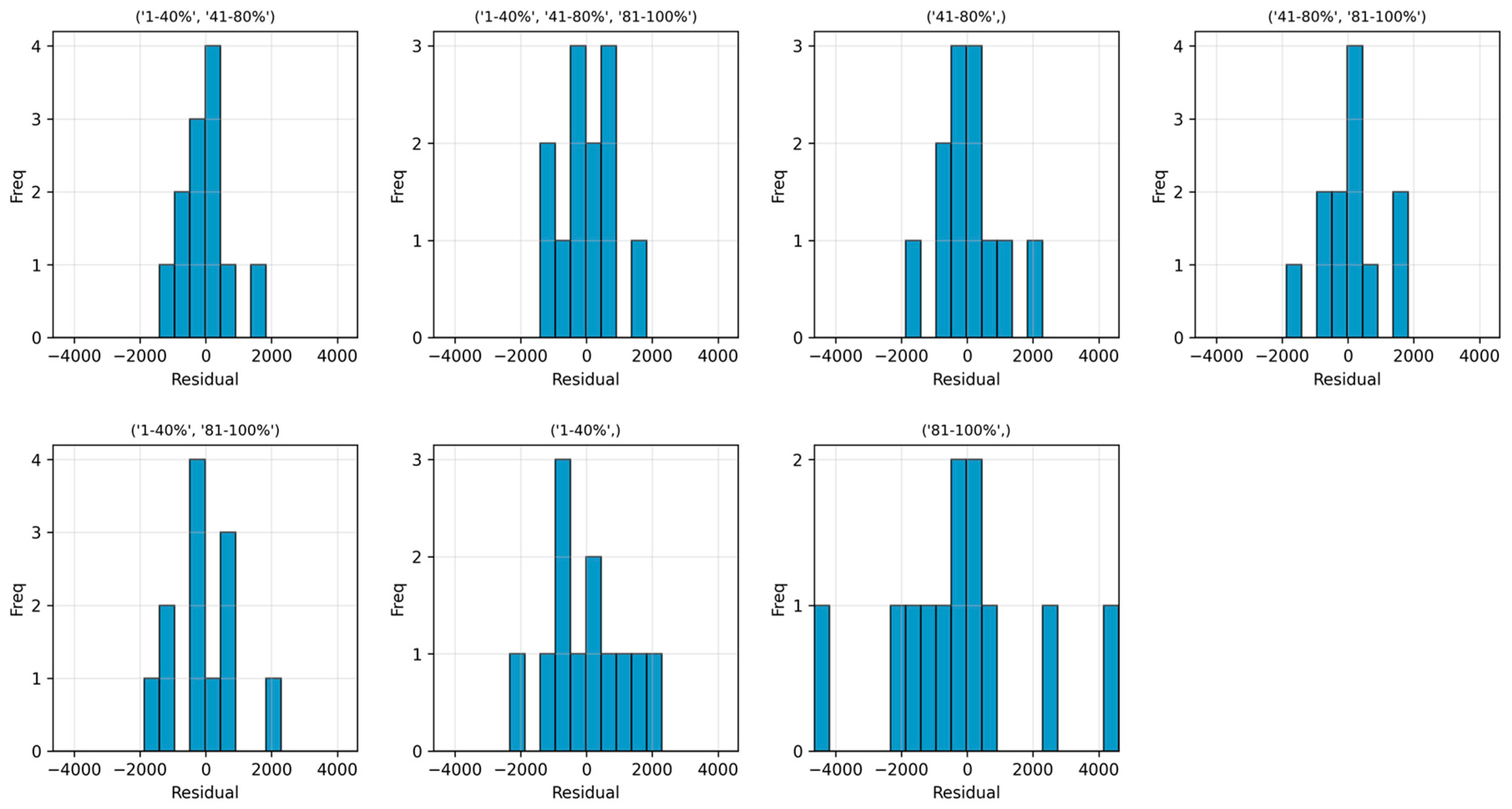
3.4. Prediction and Accuracy Verification of Weekly Yield in the Following Week of Monitoring
4. Discussion
5. Conclusions
Author Contributions
Funding
Data Availability Statement
Acknowledgments
Conflicts of Interest
References
- Takayama, K.; Hirota, R.; Takahashi, N.; Yamamoto, K.; Sakai, Y.; Okada, H.; Nishina, H.; Arima, S. Development of Chlorophyll Fluorescence Imaging Robot for Practical Use in Commercial Greenhouse. Acta Hortic. 2014, 1037, 671–676. [Google Scholar] [CrossRef]
- Sun, X. Enhanced Tomato Detection in Greenhouse Environments: A Lightweight Model Based on S-YOLO with High Accuracy. Front. Plant Sci. 2024, 15, 1451018. [Google Scholar] [CrossRef]
- Wang, S.; Xiang, J.; Chen, D.; Zhang, C. A Method for Detecting Tomato Maturity Based on Deep Learning. Appl. Sci. 2024, 14, 11111. [Google Scholar] [CrossRef]
- Zhao, J.; Bao, W.; Mo, L.; Li, Z.; Liu, Y.; Du, J. Design of Tomato Picking Robot Detection and Localization System Based on Deep Learning Neural Networks Algorithm of Yolov5. Sci. Rep. 2025, 15, 6180. [Google Scholar] [CrossRef]
- Afonso, M.; Fonteijn, H.; Fiorentin, F.S.; Lensink, D.; Mooij, M.; Faber, N.; Polder, G.; Wehrens, R. Tomato Fruit Detection and Counting in Greenhouses Using Deep Learning. Front. Plant Sci. 2020, 11, 571299. [Google Scholar] [CrossRef]
- Rong, J.; Zhou, H.; Zhang, F.; Yuan, T.; Wang, P. Tomato Cluster Detection and Counting Using Improved YOLOv5 Based on RGB-D Fusion. Comput. Electron. Agric. 2023, 207, 107741. [Google Scholar] [CrossRef]
- Naito, H.; Shimomoto, K.; Fukatsu, T.; Hosoi, F.; Ota, T. Interoperability Analysis of Tomato Fruit Detection Models for Images Taken at Different Facilities, Cultivation Methods, and Times of the Day. AgriEngineering 2024, 6, 1827–1846. [Google Scholar] [CrossRef]
- Shimomoto, K.; Naito, H.; Fukatsu, T.; Ota, T. Development of an AI-Based Fruit Monitoring System with a Focus Illumination Unit for Tomatoes Grown in Greenhouse Horticulture. Eng. Agric. Environ. Food 2025, 18, 23–31. [Google Scholar] [CrossRef]
- Naito, H.; Ota, T.; Shimomoto, K.; Hosoi, F.; Fukatsu, T. Accuracy Assessment of Tomato Harvest Working Time Predictions from Harvestable Fruit Counts in Panoramic Images. Agriculture 2024, 14, 2257. [Google Scholar] [CrossRef]
- Nuske, S.; Wilshusen, K.; Achar, S.; Yoder, L.; Narasimhan, S.; Singh, S. Automated Visual Yield Estimation in Vineyards. J. Field Robot. 2014, 31, 837–860. [Google Scholar] [CrossRef]
- Stein, M.; Bargoti, S.; Underwood, J. Image Based Mango Fruit Detection, Localisation and Yield Estimation Using Multiple View Geometry. Sensors 2016, 16, 1915. [Google Scholar] [CrossRef]
- Sabir, N.; Singh, B. Protected Cultivation of Vegetables in Global Arena: A Review. Indian J. Agric. 2013, 83, 123–135. [Google Scholar]
- Moon, T.; Park, J.; Son, J.E. Prediction of the Fruit Development Stage of Sweet Pepper (Capsicum annuum var. annuum) by an Ensemble Model of Convolutional and Multilayer Perceptron. Biosyst. Eng. 2021, 210, 171–180. [Google Scholar] [CrossRef]
- Viveros Escamilla, L.D.; Gómez-Espinosa, A.; Escobedo Cabello, J.A.; Cantoral-Ceballos, J.A. Maturity Recognition and Fruit Counting for Sweet Peppers in Greenhouses Using Deep Learning Neural Networks. Agriculture 2024, 14, 331. [Google Scholar] [CrossRef]
- Hemming, J.; Bac, C.W.; van Tuijl, B.A.J.; Barth, R.; Bontsema, J.; Pekkeriet, E.J.; van Henten, E.J. A Robot for Harvesting Sweet-Pepper in Greenhouses. In Proceedings of the International Conference of Agricultural Engineering, Zurich, Switzerland, 6–10 July 2014. [Google Scholar]
- Bac, C.W.; Hemming, J.; van Tuijl, B.A.J.; Barth, R.; Wais, E.; van Henten, E.J. Performance Evaluation of a Harvesting Robot for Sweet Pepper. J. Field Robot. 2017, 34, 1123–1139. [Google Scholar] [CrossRef]
- Lehnert, C.; McCool, C.; Sa, I.; Perez, T. A Sweet Pepper Harvesting Robot for Protected Cropping Environments. arXiv 2018, arXiv:1810.11920. [Google Scholar]
- Arad, B.; Balendonck, J.; Barth, R.; Ben-Shahar, O.; Edan, Y.; Hellström, T.; Hemming, J.; Kurtser, P.; Ringdahl, O.; Tielen, T.; et al. Development of a Sweet Pepper Harvesting Robot. J. Field Robot. 2020, 37, 1027–1039. [Google Scholar] [CrossRef]
- Heuvelink, E.; Marcelis, L.F.M.; Körner, O. How to Reduce Yield Fluctuations in Sweet Pepper? Acta Hortic. 2004, 633, 349–355. [Google Scholar] [CrossRef]
- Heuvelink, E.; Marcelis, L.; Kierkels, T. Young Fruits Pull so Hard Flowers Above Abort. Wagening. Univ. Res. 2016, 5, 16–17. [Google Scholar]
- Homma, M.; Watabe, T.; Ahn, D.-H.; Higashide, T. Dry Matter Production and Fruit Sink Strength Affect Fruit Set Ratio of Greenhouse Sweet Pepper. J. Am. Soc. Hortic. Sci. 2022, 147, 270–280. [Google Scholar] [CrossRef]
- Shinozaki, Y.; Nicolas, P.; Fernandez-Pozo, N.; Ma, Q.; Evanich, D.J.; Shi, Y.; Xu, Y.; Zheng, Y.; Snyder, S.I.; Martin, L.B.B.; et al. High-Resolution Spatiotemporal Transcriptome Mapping of Tomato Fruit Development and Ripening. Nat. Commun. 2018, 9, 364. [Google Scholar] [CrossRef]
- Harel, B.; van Essen, R.; Parmet, Y.; Edan, Y. Viewpoint Analysis for Maturity Classification of Sweet Peppers. Sensors 2020, 20, 3783. [Google Scholar] [CrossRef]
- Kasampalis, D.S.; Tsouvaltzis, P.; Ntouros, K.; Gertsis, A.; Gitas, I.; Siomos, A.S. The Use of Digital Imaging, Chlorophyll Fluorescence and Vis/NIR Spectroscopy in Assessing the Ripening Stage and Freshness Status of Bell Pepper Fruit. Comput. Electron. Agric. 2021, 187, 106265. [Google Scholar] [CrossRef]
- Wang, L.; Zhong, Y.; Liu, J.; Ma, R.; Miao, Y.; Chen, W.; Zheng, J.; Pang, X.; Wan, H. Pigment Biosynthesis and Molecular Genetics of Fruit Color in Pepper. Plants 2023, 12, 2156. [Google Scholar] [CrossRef]
- Kurtser, P.; Edan, Y. Statistical Models for Fruit Detectability: Spatial and Temporal Analyses of Sweet Peppers. Biosyst. Eng. 2018, 171, 272–289. [Google Scholar] [CrossRef]
- Kano, T.; Toda, S.; Unno, H.; Fujiuchi, N.; Nishina, H.; Takayama, K. Development of Hanging-Type Multiple Biological Information Imaging Robot for Growth Monitoring of Tomato Plants. Eco Eng. 2022, 34, 37–44. [Google Scholar] [CrossRef]
- Matterport/Mask_RCNN. Available online: https://github.com/matterport/Mask_RCNN (accessed on 26 April 2025).
- He, K.; Gkioxari, G.; Dollár, P.; Girshick, R. Mask R-CNN. IEEE Trans. Pattern Anal. Mach. Intell. 2020, 42, 386–397. [Google Scholar] [CrossRef]
- Wang, X.; Zhang, R.; Shen, C.; Kong, T.; Li, L. SOLO: A Simple Framework for Instance Segmentation. arXiv 2020, arXiv:1912.04488. [Google Scholar] [CrossRef]
- Lin, T.-Y.; Maire, M.; Belongie, S.; Hays, J.; Perona, P.; Ramanan, D.; Dollár, P.; Zitnick, C.L. Microsoft COCO: Common Objects in Context. In Proceedings of the European Conference on Computer Vision (ECCV), Zurich, Switzerland, 6–12 September 2014. [Google Scholar]
- Aleju/Imgaug. Available online: https://github.com/aleju/imgaug (accessed on 26 April 2025).
- Jonauskaite, D.; Mohr, C.; Antonietti, J.-P.; Spiers, P.M.; Althaus, B.; Anil, S.; Dael, N. Most and Least Preferred Colours Differ According to Object Context: New Insights from an Unrestricted Colour Range. PLoS ONE 2016, 11, e0152194. [Google Scholar] [CrossRef] [PubMed]
- Ohno, H.; Sasaki, K.; Ohara, G.; Nakazono, K. Development of Grid Square Air Temperature and Precipitation Data Compiled from Observed, Forecasted, and Climatic Normal Data. Clim. Biosph. 2016, 16, 71–79. [Google Scholar] [CrossRef]
- Yue, X.; Qi, K.; Na, X.; Zhang, Y.; Liu, Y.; Liu, C. Improved YOLOv8-Seg Network for Instance Segmentation of Healthy and Diseased Tomato Plants in the Growth Stage. Agriculture 2023, 13, 1643. [Google Scholar] [CrossRef]
- Hemming, J.; Ruizendaal, J.; Hofstee, J.W.; van Henten, E.J. Fruit Detectability Analysis for Different Camera Positions in Sweet-Pepper. Sensors 2014, 14, 6032–6044. [Google Scholar] [CrossRef] [PubMed]
- Wang, X.; Vladislav, Z.; Viktor, O.; Wu, Z.; Zhao, M. Online Recognition and Yield Estimation of Tomato in Plant Factory Based on YOLOv3. Sci. Rep. 2022, 12, 8686. [Google Scholar] [CrossRef] [PubMed]
- Shimomoto, K.; Shimazu, M.; Matsuo, T.; Kato, S.; Naito, H.; Fukatsu, T. Development of double-camera AI system for efficient monitoring of paprika fruits. In Proceedings of the International Symposium on New Technologies for Sustainable Greenhouse Systems: GreenSys2023, Cancún, Mexico, 22–27 October 2023. [Google Scholar] [CrossRef]


| Color | Hue Value |
|---|---|
| Red | 0 ≤ hue < 30, 345 ≤ hue < 360 |
| Turning | 30 ≤ hue < 70 |
| Green | 70 ≤ hue < 160 |
| Week | APIoU = 0.50 |
|---|---|
| 1 | 0.71 |
| 2 | 0.71 |
| 3 | 0.73 |
| 4 | 0.77 |
| 5 | 0.72 |
| 6 | 0.76 |
| 7 | 0.76 |
| 8 | 0.74 |
| 9 | 0.73 |
| 10 | 0.71 |
| 11 | 0.74 |
| 12 | 0.73 |
| Variable Combination | Equation | WAPE |
|---|---|---|
| (‘1–40%’, ‘41–80%’) | 4 | 21.35 |
| (‘1–40%’, ‘41–80%’, ‘81–100%’) | 2 | 24.06 |
| (‘41–80%’) | 8 | 25.70 |
| (‘41–80%’, ‘81–100%’) | 5 | 28.70 |
| (‘1–40%’, ‘81–100%’) | 6 | 29.24 |
| (‘1–40%’) | 7 | 38.53 |
| (‘81–100%’) | 9 | 63.18 |
Disclaimer/Publisher’s Note: The statements, opinions and data contained in all publications are solely those of the individual author(s) and contributor(s) and not of MDPI and/or the editor(s). MDPI and/or the editor(s) disclaim responsibility for any injury to people or property resulting from any ideas, methods, instructions or products referred to in the content. |
© 2025 by the authors. Licensee MDPI, Basel, Switzerland. This article is an open access article distributed under the terms and conditions of the Creative Commons Attribution (CC BY) license (https://creativecommons.org/licenses/by/4.0/).
Share and Cite
Shimomoto, K.; Shimazu, M.; Matsuo, T.; Kato, S.; Naito, H.; Kashino, M.; Ohta, N.; Yoshida, S.; Fukatsu, T. Predicting Sweet Pepper Yield Based on Fruit Counts at Multiple Ripeness Stages Monitored by an AI-Based System Mounted on a Pipe-Rail Trolley. Horticulturae 2025, 11, 718. https://doi.org/10.3390/horticulturae11070718
Shimomoto K, Shimazu M, Matsuo T, Kato S, Naito H, Kashino M, Ohta N, Yoshida S, Fukatsu T. Predicting Sweet Pepper Yield Based on Fruit Counts at Multiple Ripeness Stages Monitored by an AI-Based System Mounted on a Pipe-Rail Trolley. Horticulturae. 2025; 11(7):718. https://doi.org/10.3390/horticulturae11070718
Chicago/Turabian StyleShimomoto, Kota, Mitsuyoshi Shimazu, Takafumi Matsuo, Syuji Kato, Hiroki Naito, Masakazu Kashino, Nozomu Ohta, Sota Yoshida, and Tokihiro Fukatsu. 2025. "Predicting Sweet Pepper Yield Based on Fruit Counts at Multiple Ripeness Stages Monitored by an AI-Based System Mounted on a Pipe-Rail Trolley" Horticulturae 11, no. 7: 718. https://doi.org/10.3390/horticulturae11070718
APA StyleShimomoto, K., Shimazu, M., Matsuo, T., Kato, S., Naito, H., Kashino, M., Ohta, N., Yoshida, S., & Fukatsu, T. (2025). Predicting Sweet Pepper Yield Based on Fruit Counts at Multiple Ripeness Stages Monitored by an AI-Based System Mounted on a Pipe-Rail Trolley. Horticulturae, 11(7), 718. https://doi.org/10.3390/horticulturae11070718