Article

Modeling Anaerobic Co-Digestion of Corn Stover Hydrochar and Food Waste for Sustainable Biogas Production

1
Bioproduction Engineering, Laboratory of Agricultural Bio-System Engineering, Graduate School of Agriculture, Hokkaido University, 9-9 Kita, Kita-ku, Sapporo 060-8589, Hokkaido, Japan
2
Research Faculty of Agriculture, Hokkaido University, 9-9 Kita, Kita-ku, Sapporo 060-8589, Hokkaido, Japan
*
Author to whom correspondence should be addressed.
Fermentation 2022, 8(3), 110; https://doi.org/10.3390/fermentation8030110
Submission received: 10 February 2022 / Revised: 28 February 2022 / Accepted: 1 March 2022 / Published: 3 March 2022
(This article belongs to the Special Issue Modeling and Simulation of Fermentation)

Abstract

:
Despite the importance of the biodegradability of lignocellulose biomass, few studies have evaluated the lignocellulose biomass digestion kinetics and modeling of the process. Anaerobic digestion (AD) is a mature energy production technique in which lignocellulose biomass is converted into biogas. However, using different organic waste fractions in AD plants is challenging. In this study, lignocellulose biomass (corn stover hydrochar) obtained from hydrothermal carbonization at a temperature, residential time, and biomass/water ratio of 215 °C, 45 min, and 0.115, respectively, was added to the bioreactor as a substrate inoculated with food waste and cow dung to generate biogas. A state–space AD model containing one algebraic equation and two differential equations was constructed. All the parameters used in the model were dependent on the AD process conditions. An adaptive identifier system was developed to automatically estimate parameter values from input and output data. This made it possible to operate the system under different conditions. Daily cumulative biogas production was predicted using the model, and goodness-of-fit analysis indicated that the predicted biogas production values had accuracies of >90% during both model construction and validation. Future work will focus on the application of modeling predictive control into an AD system that would comprise both models and parameters estimation.

1. Introduction

As the consumption of energy increases globally, fossil fuel resources decrease from overexploitation and are likely to become scarce or exhausted in future generations, therefore, developing renewable energy and alternative fuels is a promising solution to this situation [1,2]. The emissions of carbon and pollutants from the burning of fossil fuel over the years have had a great impact on the environment [3]. To reduce the overdependence on fossil fuel consumption and pollutant emissions, exploitation of renewable energy resources like wind and solar power systems is required [4]. Environmental conditions affect the amount of renewable energy produced by wind and solar power systems, which are currently the main systems generating renewable energy around the world [5,6]. These systems are referred to as variable renewable resources. To increase the supply of renewable energy, which is the key factor in the attainment of sustainable development goals, using lignocellulose biomass, which is not affected by environmental change, as a renewable and sustainable resource is necessary [5]. The production of lignocellulosic biomass is estimated to be 200 billion tons annually. Improper management of these lignocellulose biomass resources can pollute the environment [7,8,9]. The conversion of lignocellulose biomass into biogas is a potential alternative for green energy to meet world demand and ensure an adequate future supply of clean energy and fuel [10,11]. A system in which energy is generated from lignocellulose biomass would be robust and could compensate for fluctuations in the outputs of other renewable energy resources. AD can be applied to convert lignocellulose biomass to biogas, and it is also an important technique because it concurrently recovers energy and treats waste [12,13]. Additionally, the digestate by-product of AD can be utilized as a soil improver.
The numerical optimization of the AD process has been extensively studied for bioenergy production and wastewater treatment because of its ability to convert energy crops or organic waste into biogas in the absence of oxygen [14]. The anaerobic transformation of organic matter is a complex biochemical process involving numerous bacterial populations, which make the process nonlinear, uncertain, and therefore difficult to predict and simulate. For this purpose, the design, modeling, and simulation of the AD process have attracted much attention over the decades. As a basis for modeling and simulating the AD process, many mathematical models have been established and used to identify ways of decreasing operating costs and improving process stability. Reference [15] utilized a dynamic model to improve the process stability of AD by regulating the concentration of volatile fatty acid and total alkalinity, which are inhibitors of the process. In addition, a feeding management strategy to compensate for the variation between demand and supply of energy production was established by [16]. Therefore, AD can be utilized to benefit energy demand and supply regulations, and the models can facilitate exact prediction of biogas generation and offer flexibility and robustness under different operating conditions. In terms of practicability, a model for controlling biological variables such as substrate concentration, bacterial concentration, and product (biogas production) is still being developed [17,18]. This is because these variables involve living organisms whose behavior is dynamic, nonstationary, and nonlinear. There is also the lack of a cheap sensor that can efficiently offer reliable online measurement of the biochemical parameters that is needed to execute high performance of computer control strategies. It is time-consuming to experimentally ascertain all the biochemical parameters and constants involved in ADM1 for each operating condition when a simplified model for the prediction of biogas generation can be devised. Regarding the practicability at the commercial scale of a biogas plant, a simplified model of biogas production and a parametric study of the model constants were established by [14,17,19,20,21,22,23]. The kinetic parameters in these simplified models vary drastically because of the abstract reaction dynamics, wherein some parameters were obtained from the literature while other were determined by conducting series of experiments [24], and this makes it difficult to effectively determine the values of the parameters, which hinders the use of this model in the control process. Reference [5] established another simplified model for biogas production and developed an adaptive identifier system to estimate parameters from data acquired while a process is being performed. This adaptive identifier system has a control signal with asymptotic functions of real and equal roots, meaning there is only one tuning parameter. This makes estimating the parameters, controlling the process, and predicting biogas production possible. In this study, the asymptotic function of the control signal was modified to have real and unequal roots, meaning there are two tuning parameters that make it flexible for adjustment. However, to the best of the authors’ knowledge, there are limited studies on modeling anaerobic co-digestion of corn stover hydrochar and food waste for sustainable biogas production.
It is possible to use AD to mitigate variations in the power outputs of other renewable energy sources because current practice is to run an AD system using the same amount of waste each day and to keep raw material input consistent. Quickly changing raw material inputs can excessively affect the fermentation state and cause poor fermentation [25]. An improved model for predicting biogas production that takes the fermentation state into account is required. A state–space model can describe an unobserved fermentation state, including substrate variables (corn stover hydrochar and food waste) and the bacterial concentration, using data from the biogas analyses. It is important to estimate the variables used in the model. The aim of this study is to develop a state–space model appropriate for controlling biogas generation and an adaptive identifier that can automatically estimate the key parameters representing the input and output characteristics of the AD process from experimental data.

2. Materials and Methods

2.1. Flow during Hydrothermal Carbonization and Anaerobic Digestion

The HTC and AD processes are shown as a flow diagram in Figure 1. The corn stover hydrochar used in the study was prepared as described in detail by [9]. The food waste used in the study was collected from a cafeteria at Hokkaido University. The food waste was ground using a food processor, then small portions were placed in bags and frozen. To prepare the feedstock, a portion of food waste (which had a high nitrogen content) was mixed with paper to achieve a C/N ratio of ~40 to decrease inhibition by ammonia, which can be caused by AD of N-rich feedstock [5,26]. Corn stover hydrochar was then mixed with the ground food waste at a mass ratio of 2:1. The prepared feedstock was then placed in a horizontal cylindrical bioreactor (effective volume 0.235 m3), which was kept at ~52 °C and stirred frequently to allow degassing and to ensure that the feedstock was adequately mixed.
The generated biogas was determined hourly using a wet gas meter (W-NKDa-0.5B; SHINAGAWA, Tokyo, Japan) and recorded using a data logger (Data mini LR 5000; HIOKI, Tokyo, Japan). Some digestate was collected when the feedstock was added and the remaining digestate (excluding the returned digestate) was treated as surplus. The volatile compound and total solid contents of the feedstock were ~35 and ~40%, respectively. The sludge in the reactor remained at the thermophilic temperature of 52 °C. The HTC and AD processes were therefore classed as dry thermophilic techniques that would minimize digestate emissions because no water needed to be added.

2.2. State–Space Model of AD

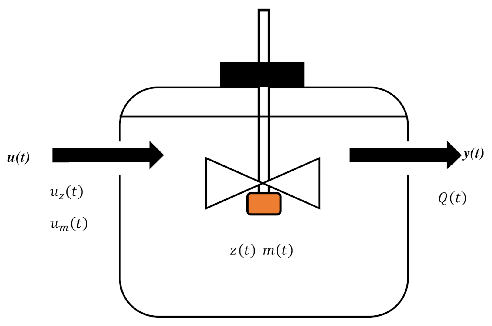
Some assumptions about the AD process were made to simplify the model development. The reactions that converted the input organic components (the substrate) to the output (biogas) were included in the model. A semi-batch bioreactor was used, and the sludge was completely mixed. The volume of sludge in the bioreactor was kept constant at 0.2. The substrate concentration m t and bacteria concentration z t were the state variables that characterized fermentation in the bioreactor. The substrate and bacteria concentrations in the feedstock were treated as manipulated variables u z t and u m t , respectively, and the biogas concentration was treated as the control variable Q t . The simplified bioreactor using these variables is shown in Figure 2. The mathematical AD model was built based on mass balance theory.
The state equation consisted of two differential equations, one for bacterial growth and the other for substrate disintegration. A logistic difference equation was used to indicate bacterial growth because it is an efficient equation used in population biology [21]. The substrate disintegration equation was used to indicate substrate degradation in line with bacterial growth. The output equation was used to describe the biogas flow rate caused by biogas production through substrate decay and bacterial growth [27]. The growth rates used in these equations were given by a modified Monod equation [28]. The mathematical model of AD was constructed by concatenating the two differential equations and one algebraic equation, as shown in Equation (1):
dz t dt μ m     a z t 1 z t z max   +   u z t dm t dt = 1 w μ m z t   +     u m t y t   =   Lq 1   1 w μ m   +   Lq 2 a vz t  
μ m   =   μ max m t K s + m t   +   bm 2 t  
In Equation   1 , z t is the bacteria concentration ( kg / m 3 ), m t is the substrate concentration ( kg / m 3 ), y(t) is the gas generation rate ( m 3 / h ), u z t is bacterial input ( kg / ( m 3   h ), u m t is substrate input ( kg / ( m 3   h ), μ m is the specific growth rate ( h 1 ), a is the autolysis rate ( h 1 ), z m a x is the bacteria-carrying capacity ( kg / m 3 ), w is the bacterial cell yield, L q 1 and L q 2 are gas generation coefficients, v is the sludge volume ( m 3 ), b is the inhibition coefficient, K s is the dissociation constant ( kg / m 3 ), and μ m a x is the maximum specific growth rate (h−1)
Perturbation theory was applied near the point at which equilibrium was reached using the nonlinear model by ignoring the second order and higher-order terms after Taylor expansion of the two-variable functions, as shown in Equations (2) and (5), to give the linear-time state–space model shown in Equation (6). The method described next was used to derive Equation (6). First, temporal changes in the state and the output variables of the AD system were considered using Equation (6).
The method described next was used to derive Equation (6). First, temporal changes in the state and the output variables of the AD system were considered using Equation (6):
dX t dt = F X t , U t , t  
  y t   =   g X t , t
Assuming that the reactions were near equilibrium, Equation (2) was transformed into Equation (3):
dX t dt =   F X eq +   X t ,   U eq +   U t , t   y t   =   g X eq +   X t , t
In Equation (3), X e q ,   U e q is the equilibrium point and X t , U t is the perturbation. The right-hand side of Equation (3) was rewritten by ignoring the second-order and higher-order terms after Taylor series expansion of the two variables to give Equation (4):
F X eq +   X t ,   U eq +   U t , t     F X eq , U eq , t     +     X t X t +   U t U t F X t , U t , t X eq , U eq , t
y t   = g X eq   +   X t g X t X eq ,   t
Finally, Equation (6) was obtained by substituting the equilibrium point in Equation (4) into Equation (5):
dX t dt = F X t X eq , U eq , t X t   +   F X t X eq , U eq , t U t  
y t   = g X t X eq , t X t
The substitution above gave Equation (2) in the form:
dX t dt = A q X t   +   B q U t
y t   = C q X t
A q = F X t X eq , U eq , t =   a 11 a 12 a 21 a 22
B q = F U t X eq , U eq , t =   b 11 b 12 b 21 b 22
C q = g X t X eq , t =   c 11 c 12 ,
where a 11 , a 12 , a 21 , a 22 , b 11 , b 12 , b 21 , b 22 , c 11 , and   c 12 are all Jacobian elements:
f 1 X t , U t , t ;   dz t dt =   μ m     a z t 1 z t z max +   u z t
f 2 X t , U t , t ;   dm t dt = 1 w μ m z t   +   u m t
g X t , t ; Q t   =   Lq 1 1 w μ m   +   Lq 2 a vz t
F X t , U t ,   t   =   f 1 X t , U t , t f 2 X t , U t , t
X t therefore, represents matrices containing coefficients of the vectors of the state variables and U t represents the vectors of the manipulated variables that are partial derivative matrices for the equilibrium point of the Jacobian matrix. These parameters provide information about the characteristics of the AD process under the relevant operating conditions.

Parameter Estimation System

A z-transformation was performed on the state–space model to give the discrete input and output relational expressions shown in Equation (10) taking Equations (7)–(9) into consideration. This is equivalent to performing the Laplace transformation for discrete time but replacing the operator in the Laplace transformation with a delay operator. The z-transformation of Equation (6) is shown in Equation (7):
q 1 X p   = A q X t   +   B q U t  
y p   = C q X p ,
where q 1 is the delay operator.
The coefficient of the variable on the left-hand side of Equation (7) is a scalar variable, so Equation (8) was derived from Equation(7):
X p   = q 1 I A q 1 B q U t   +   X 0
y p   = C q X p  
The initial value was therefore not considered in this study and Equation (10) was obtained by combining the two expressions shown in Equation (8) as shown below:
y p   = C q q 1 I A q 1 B q U t  
where:
q 1 I A q 1 = adj q 1 I A q det q 1 I A q = 1 q 2   +   a 11   a 22 q 1   +   a 11 a 22     a 12 a 21   q 1 a 22 a 12 a 12 q 1 a 11 A q y p   =   B q U p  
where:
A q   =   q 2 +   a 11 a 22 q 1 +   a 11 a 22 a 12 a 21   =   q 2 + a 1 q 1 +   a 2
and:
B q   =   c 11 q 1 a 22   +   c 12 a 21   c 11 a 12 +   c 12 q 1   a 11 =   b 1 q 1 + b 2   b 3 q 1 + b 4
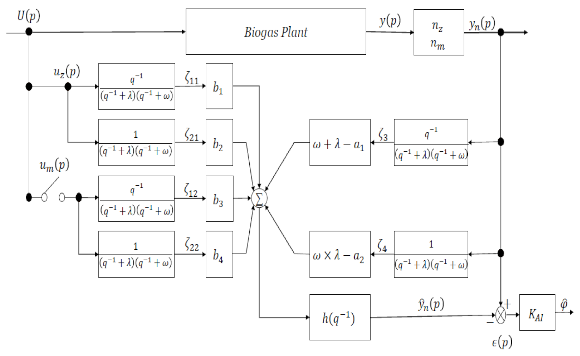
The original parameters of the model shown in Equation (6) were changed to a 1 ,   a 2 and b 1 ,   b 2 ,   b 3 ,   b 4 . Once the values had been estimated, biogas generation y p could be predicted by inputting the bacteria and substrate concentrations in the feedstock U k into Equation (10). An adaptive identifier was developed using the adaptive identification theory to estimate the parameters from real operational data [5,29]. The adaptive identifier shown in Figure 3 was used as the control system. Input and output data were multiplied by the filter to produce the control signals ζ 11 ,   ζ 12 ,   ζ 21 ,   ζ 22 ,     ζ 3 ,   and   ζ 4 in the adaptive identifier. The control signals were multiplied by the operating parameters and then integrated, and the linear relationship between output and the parameters with the proportionality constant as the control signal was derived using Equation (11):
y p   = h q φ T ψ p  
φ T = b 1 ,   b 2 ,   b 3 ,   b 4 , ω + λ a 1 , ω × λ a 2 T  
ψ p   =   ζ 11 p , ζ 12 p , ζ 21 p , ζ 22 p , ζ 3 p , ζ 4 p
The mechanism involved in the operation of the adaptive identifier is shown in Figure 3 was verified using Equation (4):
y p   = h q ( b 1 ζ 11 p   +   b 3 ζ 12 p   +   b 2 ζ 21 p   +   b 4 ζ 22 p + ω + λ a 1 ζ 3 p + ω × λ a 2 ζ 4 p )
y p   = h q ( b 1 q 1 q 1   +   λ q 1   +   ω u z p   +   b 3 1 q 1   +   λ q 1   +   ω u z p +   b 2 q 1 q 1   +   λ q 1   +   ω u m p +   b 4 1 q 1   +   λ q 1   +   ω u m p +   ω + λ a 1 q 1 q 1   +   λ q 1   +   ω y p +   ω × λ a 2 1 q 1   +   λ q 1   +   ω y p ) = h q ( b 1 q 1   +   b 3 q 1   +   λ q 1   +   ω u z p   +   b 2 q 1   +   b 4 q 1   +   λ q 1 + ω u m p + ω   +   λ q 1 a 1   +   ω   ×   λ     a 2 q 1   +   λ q 1   +   ω y p )
The parameters used in Equation (10) were integrated into φ using Equation (11). If the matrix element values were obtained as described above, the amount of biogas generated could be predicted using Equation (10). The difference between the measured output value and the value calculated using the estimated parameters was defined as the output error ϵ p and calculated using Equation (13):
ϵ p   =   y p     h q φ T ψ p  
The recursive least-squares algorithm was applied to Equation (13) with m datasets representing inputs and outputs assuming that the estimated parameters with minimized errors were valid. The least-squares estimates of the parameters were obtained using Equation (14): where:
Y m = y 1       y 2             y m T  
and:
ψ m = ψ 1       ψ 2         ψ m T  
The parameters b 1 , b 2 , b 3 , b 4 , a 1 and a 2 were determined using the recursive least-squares algorithm, then the roots and coefficients of Equation (10) for the system were estimated using the stepwise function shown in Equation (15):
y t   =   Kz 1 e α t τ + Kz 2 e β ( t τ u z   +   Km 1 e α t τ + Km 2 e β t τ u m ,           if       a 1 2 4 a 2   > 0 Kz 1 + Kz 2 e α t τ u z   +   Km 1 + Km 2 e α t τ u m ,       if   a 1 2 4 a 2 = 0 , Kz 1 e α t τ cos ω t τ   +   Kz 2 e β t τ sin ω t τ u z + Km 1 e α t τ cos ω t τ   +   Km 2 e β t τ sin ω t τ u m ,         if   a 1 2 4 a 2   < 0
For Equation (16), if the discriminant function is a 1 2 4 a 2 > 0 , the α, β, K z 1 , and K z 2 values can be calculated using the following equations:
      α = a 1 + a 1 2 4 a 2 2 ;   β = a 1 a 1 2 4 a 2 2 ;   Kz 1 = b 1 α + b 2 α β ; Kz 2 = b 1 β + b 2 β α ;   Km 1 = b 3 α + b 4 α β   and   Km 2 = b 3 β + b 4 β α  
and if the discriminant function is a 1 2 4 a 2 < 0 , the α, ω, K z 1 , and K z 2 values can be calculated using the equations:
α   = a 1 2   ;   ω = a 1 2 4 + a 2   ;   Kz 1 = b 1   ;   Kz 2 = b 2   ;   Km 1 = b 3   and   Km 2 = α b 3 + b 4 α  
where τ   is a time constant, α , β are the roots of the function and K z 1 ,   K z 2 ,   K m 1 ,   and   K m 2 are coefficients related to the bacteria and substrate concentrations.
Therefore, the bacterial and substrate solutions for the AD system were deduced, from Equation (15), to be Equations (16) and (17), respectively:
y z model =   Kz 1 e α t τ + Kz 2 e β ( t τ u z  
y m model =   Km 1 e α t τ + Km 2 e β t τ u m  
In Equations (16) and (17), y z m o d e l and y m m o d e l are the amounts of biogas generated calculated from the bacterial and substrate concentrations, respectively.
The goodness-of-fit index (GFI) shown in Equation (18) [5] was used to quantify the accuracy of the model predictions using the estimated parameters:
GFI   %   = 100 1 y p   y ^ p y p mean y
The adaptive identifier included a switch relating to substrate inputs because the AD process had two inputs and one output. This allowed all the parameters to be estimated with or without substrate input data. The filter h q 1 , scaling coefficients n z and n m , and control system design constants λ and ω were tuned to give the desired estimates.

3. Results and Discussion

Table 1 shows the tuning constants of the adaptive identifier, h q 1 is the filter, n z and n m are scaling coefficients related to the bacteria and substrate outputs, respectively, λ and ω are control system design constants.

3.1. Simulation Data

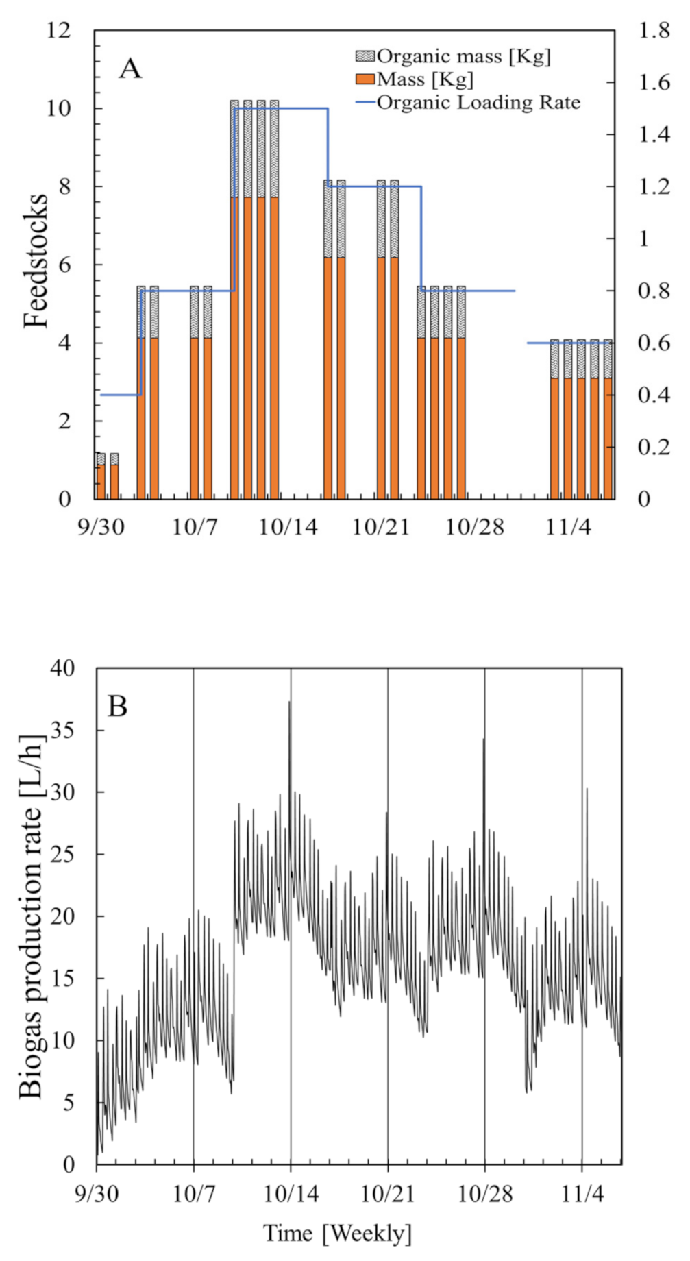
The substrate concentration was determined from the loss of mass when the feedstock was heated to 105 °C for 24 h and then to 600 °C for 3 h. The data used in the simulation were experimental data collected in the laboratory in 2018 (Figure 4). Bacterial input at 0 h was defined as the amount of substrate in the digestate at the beginning of the process [30]. Feedstock input was determined at 0, 52, and 104 h. Data for 3 d (i.e., 72 h) from 30 September 2018, when no feedstock was added, and for 7 d (i.e., 168 h) from 7 October 2018, when feedstock was added, were used to estimate the parameters when developing the model. Data for 7 d (i.e., 168 h) from 21 October 2018 were used to validate the model. The organic loading rates for the model construction period and the model validation period were different at 1.47 and 1.24 (kg volatile solid)/(m3 digester/day), respectively.

3.2. Adaptive Identifier System

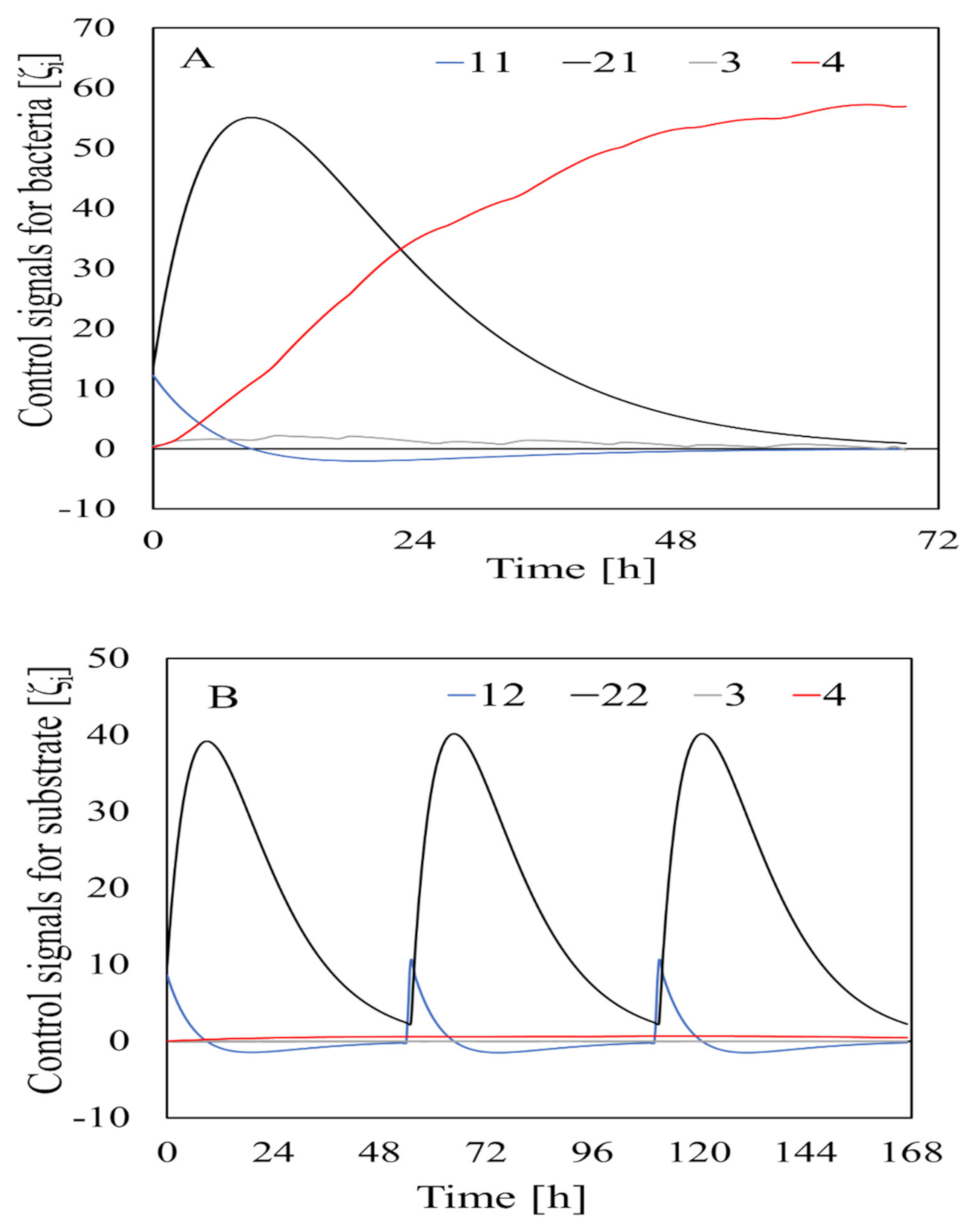
The tuning constants for the control system when the adaptive identifier was used to generate the control signals (which are shown in Figure 5) are shown in Table 1. The bacterial and substrate inputs appeared as several pulse–wave signals because the AD flow used a semi-continuous system. As shown in Figure 4, the pulse–wave input signals were converted into a control signal that changed continually according to the input.

3.3. Parameter Estimation of Bacteria and Substrate Input

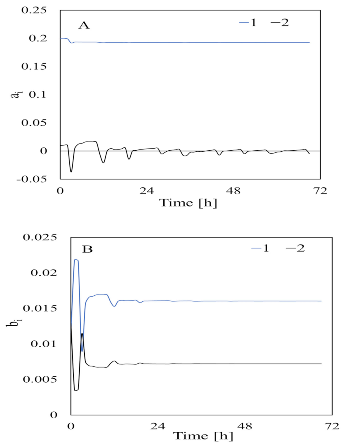
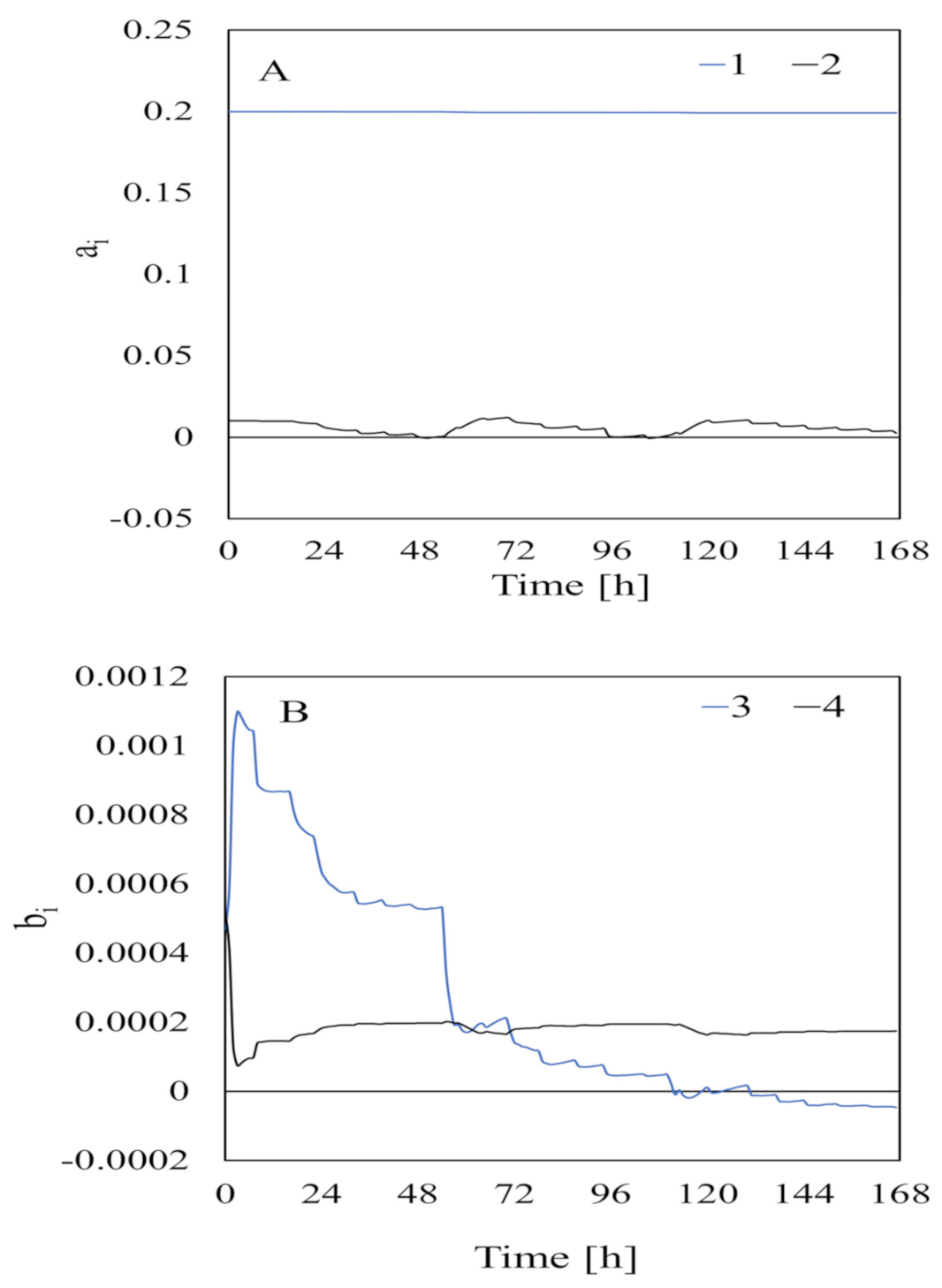
The parameters estimated using data collected when the feedstock had not been added are shown in Figure 6. The estimated parameters were very variable at first but slowly stabilized as the acquired data increased and became stable at ~20 h [5]. This indicated that data needed to be collected for at least 20 h to estimate the parameters related to bacterial input. The parameters estimated from data collected when the feedstock had been added (i.e., for identification of adaptation caused by “turning on the switch” by adding substrate) are shown in Figure 7. The parameter estimates varied greatly at the beginning of the experiment but became stable at 140 h. Therefore, data needed to be collected for at least 140 h to estimate the parameters related to substrate input. This was slightly different from the time found by [5] after assessing the composition of the substrates in a bioreactor.

3.4. Biogas Prediction Model

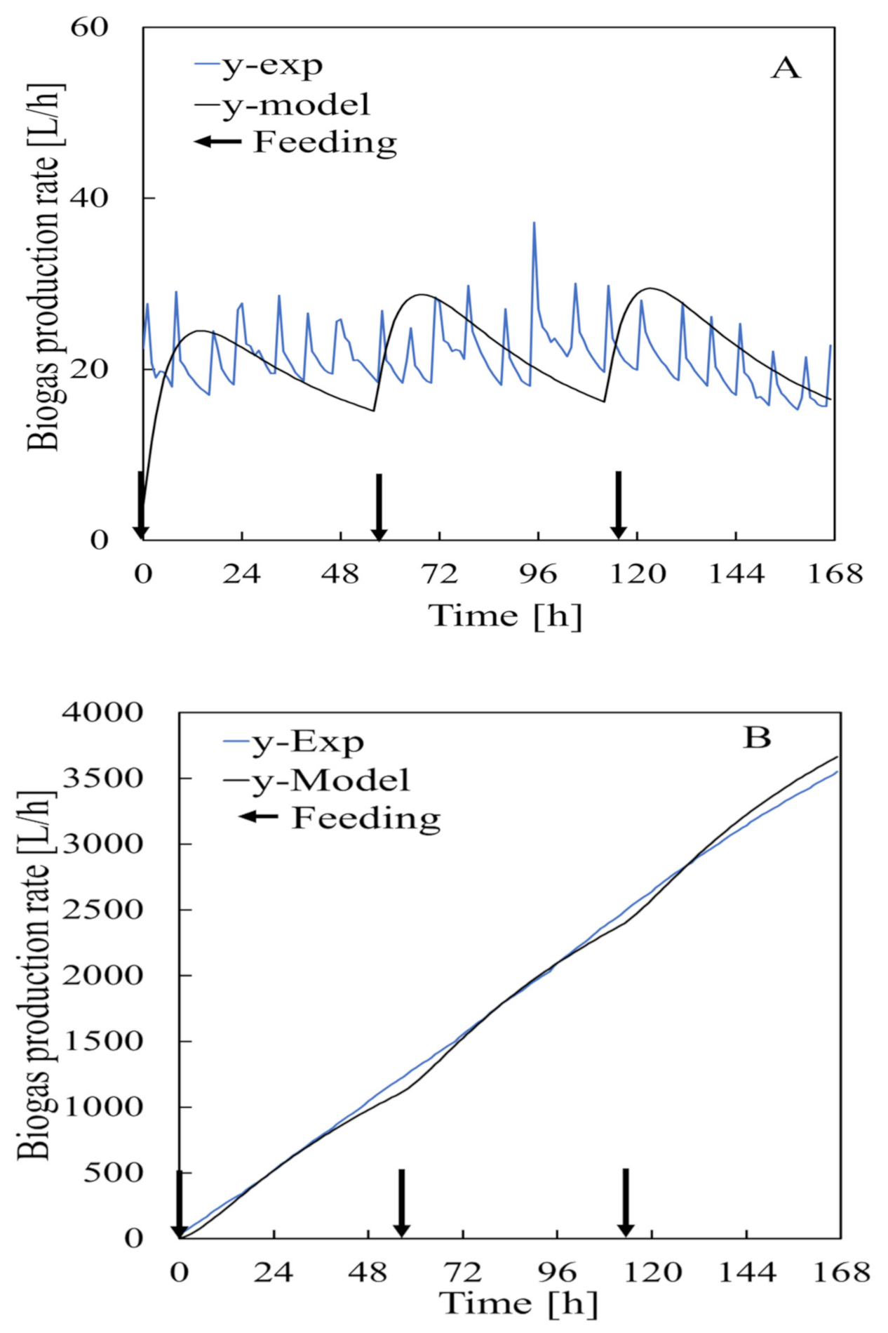
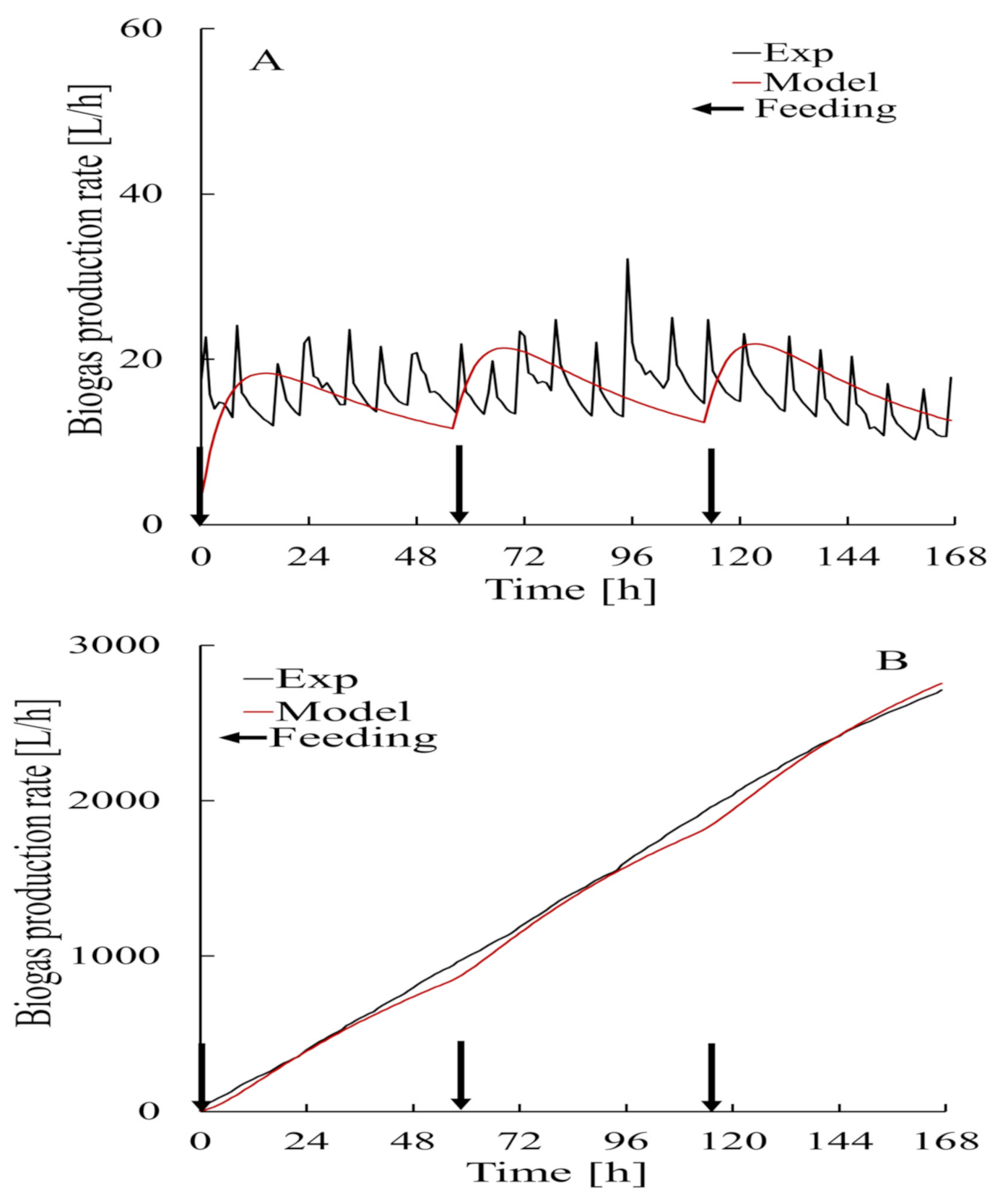
Biogas predictions made using a model constructed with the estimated parameters for the bacteria and substrate are shown in Figure 8 and Figure 9 using models (I) and (II) for cumulative biogas generation. The bacteria and substrate models did not effectively predict the amount of biogas inside the bioreactor because of the disturbance caused by agitation (stirring) and inhibition likely to slow down degradation of the substrate while the cumulative biogas generation by the models revealed high prediction accuracy.
The results of the validation tests performed using different data from the data used to construct the model are shown in Figure 10. These were carried out to confirm the accuracy of the prediction model. The initial bacteria concentrations for the period in which the data used to construct the model were acquired (30 September 2018 to 7 October 2018) and for the period in which the data used to validate the model were acquired (14–21 October 2018) were different. The initial bacteria concentration for 30 September 2018 to 7 October 2018 was 28 kg/m3 and the initial bacteria concentration for 14–21 October 2018 was 25 kg / m 3 . The amount of biogas generated that was predicted using the validation data had a low GFI (−81.91%) because degassing (caused by agitation) and heating strongly affected the hourly data. Cumulative biogas generation data are shown in Figure 10. This indicated that the predictions were good.
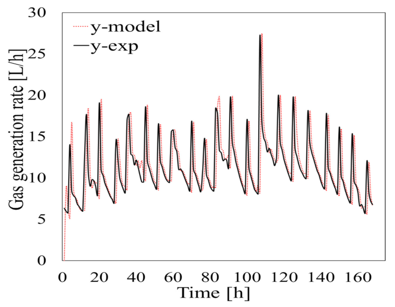
The GFI for the data set was 97.45%. The simulation results acquired using Equation (12) are shown in Figure 11. The model correctly reproduced the dynamics of the system for the test periods, although there was some variability. At the beginning of the test period the amount of biogas generated was underestimated by the model because of destabilization, but the amount of biogas generated stabilized over time and the predictions became good. The GFI for the cumulative amount of biogas generated per day is shown in Figure 12. The predicted amount was >80% of the actual amount even at the lowest value except on day 4 of period 3, which started on 14 October 2018. This indicated that the parameter estimation system and model developed in this study gave very accurate predictions for periods of 1 d or more. The parameter estimation system and model could therefore be used to predict biogas generation during AD under various operating conditions. For a real plant it would, however, be necessary to continually consider variations in operating conditions such as the feedstock composition. This could be overcome by introducing an oblivion factor to limit input data for the parameter estimation system to, for example, only the last 72 h. Estimated parameters would therefore be adaptively controlled in response to changes in the operating conditions to allow the amount of biogas produced to be predicted accurately.

4. Conclusions

The aim of this study was to develop an adaptive identifier system of the anaerobic digestion process for sustainable biogas production to allow renewable energy supplies to be stabilized. A model and parameter estimation system were established for AD processes with various operating conditions. The adaptive identifier control system automatically estimated parameters from input and output data. Using the adaptive identifier indicated that data for at least 20 and 140 h were required to estimate stable parameters related to bacterial and substrate inputs, respectively. The model and estimated parameters made accurate predictions of biogas production. Future work should be focused on constructing sustainable biogas production systems integrating predictive model biogas generation control. Such systems would allow renewable energy to be stabilized.

Author Contributions

Conceptualization, I.S.M. and N.S.; methodology, I.S.M. and R.N.; software, I.S.M.; validation, I.S.M. and N.S.; formal analysis, I.S.M.; investigation, I.S.M. and N.S.; resources, I.S.M. and N.S.; data curation, R.N. and N.S.; writing—original draft preparation, I.S.M.; writing—review and editing, I.S.M. and N.S.; visualization, I.S.M. and N.S.; supervision, N.S.; project administration, N.S.; funding acquisition, N.S. All authors have read and agreed to the published version of the manuscript.

Funding

This research was funded by a DX doctoral fellowship, Hokkaido University, Sapporo, Japan, grant number JPMJS2119, year 2021.

Institutional Review Board Statement

Not applicable.

Informed Consent Statement

Not applicable.

Data Availability Statement

Not applicable.

Acknowledgments

We thank Gareth Thomas for editing a draft of this manuscript.

Conflicts of Interest

The authors declare no conflict of interest.

References

  1. Wang, F.; Ouyang, D.; Zhou, Z.; Page, S.J.; Liu, D.; Zhao, X. Lignocellulosic biomass as sustainable feedstock and materials for power generation and energy storage. J. Energy Chem. 2020, 57, 247–280. [Google Scholar] [CrossRef]
  2. Wu, Z.; Xia, X. Optimal switching renewable energy system for demand side management. Sol. Energy 2015, 114, 278–288. [Google Scholar] [CrossRef] [Green Version]
  3. Kambo, H.S.; Dutta, A. Strength, storage, and combustion characteristics of densified lignocellulosic biomass produced via torrefaction and hydrothermal carbonization. Appl. Energy 2014, 135, 182–191. [Google Scholar] [CrossRef]
  4. Esen, M.; Yuksel, T. Experimental evaluation of using various renewable energy sources for heating a greenhouse. Energy Build. 2013, 65, 340–351. [Google Scholar] [CrossRef]
  5. Yoshida, K.; Kametani, K.; Shimizu, N. Adaptive identification of anaerobic digestion process for biogas production management systems. Bioprocess Biosyst. Eng. 2019, 43, 45–54. [Google Scholar] [CrossRef]
  6. Hamed, T.A.; Alshare, A. Environmental Impact of Solar and Wind energy—A Review. J. Sustain. Dev. Energy Water Environ. Syst. 2022, 10, 1090387. [Google Scholar] [CrossRef]
  7. Liang, J.; Nabi, M.; Zhang, P.; Zhang, G.; Cai, Y.; Wang, Q.; Zhou, Z.; Ding, Y. Promising biological conversion of lignocellulosic biomass to renewable energy with rumen microorganisms: A comprehensive review. Renew. Sustain. Energy Rev. 2020, 134, 110335. [Google Scholar] [CrossRef]
  8. Zhang, H.; Zhang, P.; Ye, J.; Wu, Y.; Fang, W.; Gou, X.; Zeng, G. Improvement of methane production from rice straw with rumen fluid pretreatment: A feasibility study. Int. Biodeterior. Biodegrad. 2016, 113, 9–16. [Google Scholar] [CrossRef]
  9. Mohammed, I.; Na, R.; Kushima, K.; Shimizu, N. Investigating the Effect of Processing Parameters on the Products of Hydrothermal Carbonization of Corn Stover. Sustainability 2020, 12, 5100. [Google Scholar] [CrossRef]
  10. Salman, C.A.; Schwede, S.; Thorin, E.; Yan, J. Enhancing biomethane production by integrating pyrolysis and anaerobic digestion processes. Appl. Energy 2017, 204, 1074–1083. [Google Scholar] [CrossRef]
  11. Mohammed, I.S.; Aliyu, M.; Abdullahi, N.A.; Alhaji, I.A. Production of Bioenergy from Rice-Melon Husk Co-Digested with Cow Dung as Innoculant. Agric. Eng. Int. CIGR J. 2020, 22, 108–117. [Google Scholar]
  12. Luz, F.C.; Volpe, M.; Fiori, L.; Manni, A.; Cordiner, S.; Mulone, V.; Rocco, V. Spent coffee enhanced biomethane potential via an integrated hydrothermal carbonization-anaerobic digestion process. Bioresour. Technol. 2018, 256, 102–109. [Google Scholar] [CrossRef]
  13. Song, X.; Wachemo, A.C.; Zhang, L.; Bai, T.; Li, X.; Zuo, X.; Yuan, H. Effect of hydrothermal pretreatment severity on the pretreatment characteristics and anaerobic digestion performance of corn stover. Bioresour. Technol. 2019, 289, 121646. [Google Scholar] [CrossRef] [PubMed]
  14. Kil, H.; Li, D.; Xi, Y.; Li, J. Model predictive control with on-line model identification for anaerobic digestion processes. Biochem. Eng. J. 2017, 128, 63–75. [Google Scholar] [CrossRef]
  15. Méndez-Acosta, H.; Palacios-Ruiz, B.; Alcaraz-González, V.; González-Álvarez, V.; García-Sandoval, J. A robust control scheme to improve the stability of anaerobic digestion processes. J. Process Control 2010, 20, 375–383. [Google Scholar] [CrossRef]
  16. Mauky, E.; Weinrich, S.; Nägele, H.-J.; Jacobi, H.F.; Liebetrau, J.; Nelles, M. Model Predictive Control for Demand-Driven Biogas Production in Full Scale. Chem. Eng. Technol. 2016, 39, 652–664. [Google Scholar] [CrossRef]
  17. Hassam, S.; Ficara, E.; Leva, A.; Harmand, J. A generic and systematic procedure to derive a simplified model from the anaerobic digestion model No. 1 (ADM1). Biochem. Eng. J. 2015, 99, 193–203. [Google Scholar] [CrossRef]
  18. Blumensaat, F.; Keller, J. Modelling of two-stage anaerobic digestion using the IWA Anaerobic Digestion Model No. 1 (ADM1). Water Res. 2005, 39, 171–183. [Google Scholar] [CrossRef]
  19. Lubenova, V.; Simeonov, I.; Queinnec, I. Two-step parameter and state estimation of the anaerobic digestion. IFAC Proc. Vol. 2002, 35, 455–460. [Google Scholar] [CrossRef] [Green Version]
  20. Simeonov, I.; Queinnec, I. Linearizing control of the anaerobic digestion with addition of acetate (control of the anaerobic digestion). Control Eng. Pr. 2006, 14, 799–810. [Google Scholar] [CrossRef]
  21. Mejdoub, H.; Ksibi, H. Regulation of Biogas Production Through Waste Water Anaerobic Digestion Process: Modeling and Parameters Optimization. Waste Biomass-Valorization 2014, 6, 29–35. [Google Scholar] [CrossRef]
  22. Arzate, J.A.; Kirstein, M.; Ertem, F.C.; Kielhorn, E.; Malule, H.R.; Neubauer, P.; Cruz-Bournazou, M.N.; Junne, S. Anaerobic Digestion Model (AM2) for the Description of Biogas Processes at Dynamic Feedstock Loading Rates. Chem. Ing. Tech. 2017, 89, 686–695. [Google Scholar] [CrossRef]
  23. Bernard, O.; Hadj-Sadok, Z.; Dochain, D.; Genovesi, A.; Steyer, J.-P. Dynamical model development and parameter identification for an anaerobic wastewater treatment process. Biotechnol. Bioeng. 2001, 75, 424–438. [Google Scholar] [CrossRef]
  24. Martinez, E.; Marcos, A.; Al-Kassir, A.; Jaramillo, M.; Mohamad, A. Mathematical model of a laboratory-scale plant for slaughterhouse effluents biodigestion for biogas production. Appl. Energy 2012, 95, 210–219. [Google Scholar] [CrossRef]
  25. Lauterböck, B.; Ortner, M.; Haider, R.; Fuchs, W. Counteracting ammonia inhibition in anaerobic digestion by removal with a hollow fiber membrane contactor. Water Res. 2012, 46, 4861–4869. [Google Scholar] [CrossRef] [PubMed]
  26. Nakajima, S.; Shimizu, N.; Ishiwata, H.; Ito, T. The Start-up of Thermophilic Anaerobic Digestion of Municipal Solid Waste. J. Jpn. Inst. Energy 2016, 95, 645–647. [Google Scholar] [CrossRef] [Green Version]
  27. May, R.M. Simple mathematical models with very complicated dynamics. Nature 1976, 261, 459–467. [Google Scholar] [CrossRef] [PubMed]
  28. Bastin, G.; Dochain, D. On-line estimation and adaptive control of bioreactors: Elsevier, Amsterdam, 1990 (ISBN 0-444-88430-0). xiv + 379 pp. Price US $ 146.25/Dfl. 285.00. Anal. Chim. Acta 1991, 243, 324. [Google Scholar] [CrossRef]
  29. Byrne, R.; Abdallah, C. Design of a model reference adaptive controller for vehicle road following. Math. Comput. Model. 1995, 22, 343–354. [Google Scholar] [CrossRef]
  30. Shimizu, N.; Yoshida, K. Development of an Efficient Anaerobic Co-digestion Process for Biogas from Food Waste and Paper. Environ. Control Biol. 2021, 59, 165–171. [Google Scholar] [CrossRef]
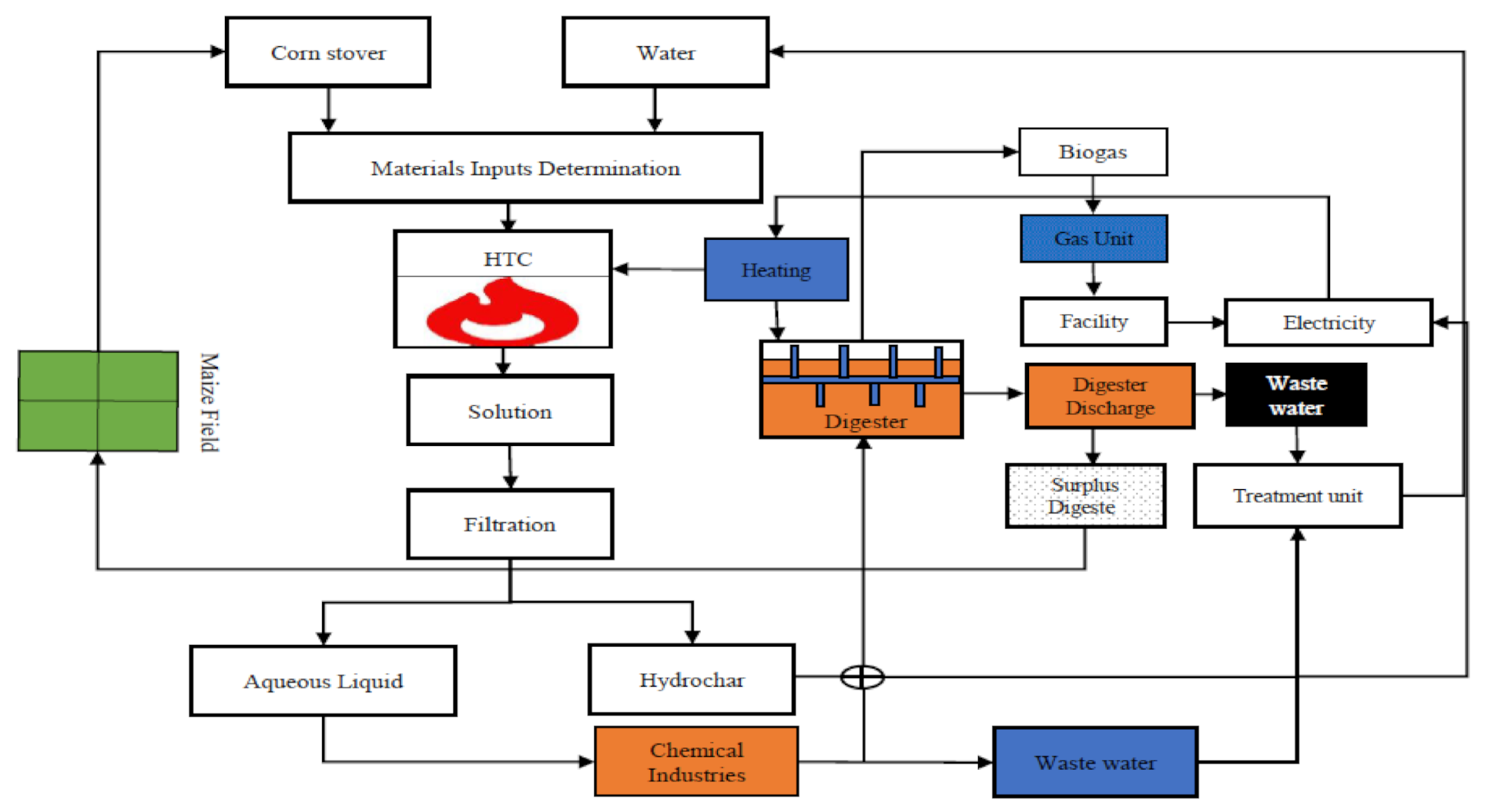
Figure 1. Hydrothermal carbonization and anaerobic digestion flow diagram. Corn stover feedstock was used to prepare hydrochar in the hydrothermal carbonization (HTC) unit, then the hydrochar was mixed with food waste and added to the anaerobic digester. Biogas was collected using a gas trap bag and the digestate from the biorefinery system was disposed of.
Fermentation 08 00110 g001
Figure 2. Graphical representation of the semi-batch-type bioreactor used for anaerobic digestion ( u z t = bacterial input (kg/(m3/h)), u m t = substrate input (kg/(m3/h)), z t = bacteria concentration (kg/m3), m t = substrate concentration (kg/m3), and Q t = biogas flow rate (m3/h)).
Fermentation 08 00110 g002
Figure 3. Adaptive identifier. U p is the feedstock input kg m 3   h ,   u z p is the bacterial input kg m 3   h , u m p is the substrate input kg m 3   h , y p is the biogas flow rate m 3 h , y n p is the scaled biogas flow rate L h , ζ 11 ,   ζ 12 ,   ζ 21 ,   ζ 22 ,   ζ 3 ,   and   ζ 4 are control signals, a 1 ,   a 2 and b 1 ,   b 2 ,   b 3 ,   b 4 are parameters, h q 1 is the filter, n z is a scaling coefficient related to the bacterial output, n m is a scaling coefficient related to the substrate output, λ   and   ω are control system design constants, y ^ n p is the predicted scaled biogas flow rate kg m 3   h , ϵ p is the error m 3 h , K A I is the coefficient for the least-squares method, and φ ^ is an estimated parameter.
Fermentation 08 00110 g003
Figure 4. Experimental data used to construct the model and perform a simulation for the feedstocks (A) and for biogas Production rate (B).
Fermentation 08 00110 g004
Figure 5. Control signals related to bacteria and substrate inputs (A) and outputs (B). ζ i is the control signal, and the numbers in the figure legends are the subscript i values for the control signals.
Fermentation 08 00110 g005
Figure 6. Estimated parameters related to bacterial input for the output side (A) and the input side (B) of Equation (10). The numbers in the legend are the subscript i values. a i is a parameter on the output side of Equation (10), and b i is a parameter on the input side of Equation (10).
Fermentation 08 00110 g006
Figure 7. Estimated parameters relating to substrate input for the output side ( A) d the input side ( B) of Equation (10). The numbers in the figure legend are the subscript i values. a i is a parameter on the output side of Equation (10) and b i is a parameter on the input side of Equation (10).
Fermentation 08 00110 g007
Figure 8. Data used to construct the model related to bacterial models (A,B) for cumulative biogas generation determined using Equation (16).
Fermentation 08 00110 g008
Figure 9. Data used to construct the model related to substrate models (A,B) for cumulative biogas generation determined using Equation (17).
Fermentation 08 00110 g009
Figure 10. Amount of biogas generated by anaerobic digestion predicted using models (A) and Cumulative (B) from data acquired from 14–21 October 2018 using Equation (15).
Fermentation 08 00110 g010
Figure 11. Experimental data and data predicted using Equation (12) plotted against time.
Fermentation 08 00110 g011
Figure 12. Goodness-of-fit values for the cumulative amount of biogas generated for each day in a 7 day period from 21 October 2018.
Fermentation 08 00110 g012
Table 1. Tuned constants for the adaptive identifier.
h(q−1)nznmλω
10.00250.00040.350.25
Publisher’s Note: MDPI stays neutral with regard to jurisdictional claims in published maps and institutional affiliations.