Article

Dynamic Optimisation of Beer Fermentation under Parametric Uncertainty

BioTeC+, Department of Chemical Engineering, KU Leuven Technology Campus Ghent, 9000 Ghent, Belgium
*
Author to whom correspondence should be addressed.
Fermentation 2021, 7(4), 285; https://doi.org/10.3390/fermentation7040285
Submission received: 4 November 2021 / Revised: 24 November 2021 / Accepted: 25 November 2021 / Published: 28 November 2021
(This article belongs to the Special Issue Implementation of Digital Technologies on Beverage Fermentation)

Abstract

:
Fermentation is one of the most important stages in the entire brewing process. In fermentation, the sugars are converted by the brewing yeast into alcohol, carbon dioxide, and a variety of by-products which affect the flavour of the beer. Fermentation temperature profile plays an essential role in the progression of fermentation and heavily influences the flavour. In this paper, the fermentation temperature profile is optimised. As every process model contains experimentally determined parameters, uncertainty on these parameters is unavoidable. This paper presents approaches to consider the effect of uncertain parameters in optimisation. Three methods for uncertainty propagation (linearisation, sigma points, and polynomial chaos expansion) are used to determine the influence of parametric uncertainty on the process model. Using these methods, an optimisation formulation considering parametric uncertainty is presented. It is shown that for the non-linear beer fermentation model, the linearisation approach performed worst amongst the three methods, while second-order polynomial chaos worked the best. Using the techniques described below, a fermentation process can be optimised for ensuring high alcohol content or low fermentation time while ensuring the quality constraints. As we explicitly consider uncertainty in the process, the solution, even though conservative, will be more robust to parametric uncertainties in the model.

1. Introduction

Consumption of alcoholic beverages like beer, wine, and spirits has always played an important role in food security and health [1]. With its history extending to more than 7 millennia [2], beer is one of the most popular beverages in the world. The global beer consumption in 2019 was estimated at around 189.05 million kilolitres [3]. The beer sector is a major contributor to the European Union’s economy with more than 10,300 active breweries providing over 130,000 jobs. In 2018, the beer sector contributed over €55 billion to the EU’s economic growth [4]. With 340 breweries in Belgium producing over 1500 different beers [5], the beer culture of Belgium has been inscribed on UNESCO’s Intangible Cultural Heritage of Humanity list [6]. According to Belgian law [7], beer is “the beverage obtained after alcoholic fermentation of a wort prepared primarily from starch and sugary raw materials, of which at least 60% barley or wheat malt, as well as hops (possibly in processed form) and brewing water”. Thus, the main ingredients which form beer are only barley malt (i.e., a starch source), hops, yeast, and water.
Nevertheless, beer production is a complex process with a multitude of processing steps involved. The barley is converted into malt during the malting process. Malting converts the hard barley grains to friable malt by producing and activating various enzymes. The malt is then milled, and mixed with water to convert the starch and proteins into fermentable sugars through a process known as mashing. The mashed product, known as wort, is then boiled with hops (although hops can be added at different stages of the beer production). The residual hops and other products coagulated from the boiling process (called the trub) are removed from the wort. The clarified wort is cooled and transferred to a fermentation tank. There it is pitched with yeast and fermented to produce ethanol, carbon dioxide, and secondary metabolites.
Although the entire process involves only four ingredients, a plethora of chemical compounds are involved in the entire brewing process. The interaction of these chemical species gives each beer its characteristic flavour. According to Amerine et al. [8], flavour is described as “the sum of perceptions resulting from stimulation of the sense ends that are grouped together at the entrance of the alimentary and respiratory tracts”. Flavour comprises (i) odour: perception of volatile compounds in the nasal cavity, (ii) aroma: perception of volatiles which pass via the nasopharyngeal passage to the olfactory epithelium, (iii) taste: perception of soluble substances on the taste buds on the surface of the tongue, and (iv) mouthfeel: physical perception of beer in the mouth [9]. Although only trace amounts of volatile esters are present in beer, they have a large influence on its flavour profile. Some common esters in beer are ethyl acetate, ethyl caprylate, ethyl octanoate, isoamyl acetate, etc. [10,11,12,13]. Apart from the esters, other volatile compounds include higher alcohols (e.g., amyl alcohol), carbonyl compounds (e.g., 2,3-butanedione, commonly called diacetyl), ketones, aldehydes, etc. [11]. Although all these compounds are produced throughout the brewing process, a majority are produced as metabolic intermediates or by-products during the fermentation step [12]. This makes fermentation a key process in the brewing chain.
Fermentation is an exothermic process in which the yeast converts the sugars in the wort to ethanol, carbon dioxide, and many other flavour-inducing compounds. The cooled wort is transferred to a cylindro-conical fermentation tank and the yeast is pitched. Along with the pitching rate and dissolved oxygen, fermentation is influenced by the temperature [14]. Temperature has a strong effect on yeast metabolism. Most brewing yeasts have optimum growth temperatures between 30 and 34 °C. However, fermentation is carried out at much lower temperatures. Typically, lagers are fermented around 10 °C, while ales are fermented at 22 °C. At elevated temperatures, the fermentation is vigorous and leads to excessive loss of volatiles and formation of undesired by-products [15]. However at higher temperatures, the time required for fermentations is reduced. Thus, the brewmaster must control the fermentation temperature such that fermentation is accelerated while still maintaining the beer quality profile. Traditionally, brewers have relied on their experience and traditional recipes for temperature control. In this paper, a computer-aided optimal control profile for the fermentation temperature is proposed.
Such an optimisation of the temperature profile is not novel. Several authors have proposed optimisation strategies to obtain a dynamic temperature profile by considering a variety of objectives. An objective describes the goal of the optimisation. In context of beer fermentation, some of the possible objectives are maximisation of ethanol concentration, minimisation of by-product formation, minimisation of batch time, or even a combination of these. Carrillo-Ureta et al. [16] used genetic algorithms to determine the temperature profiles. Their objective was the combination of five different objectives: maximise ethanol concentration, minimise two by-products, minimise batch time, and minimise jumps in the temperature profile. Xiao et al. [17] used a stochastic ant colony algorithm with similar objectives. In Rodman and Gerogiorgis [18], a weighted objective of maximum ethanol and minimum batch time was optimised using a combination of simulated annealing and high fidelity simulations. Bosse and Griewank [19] made use of forward–backward sweeping methods based on Pontryagin’s maximum principle to solve a modified version of the problem considered in Carrillo-Ureta et al. [16]. Apart from the single objective studies, several multiobjective studies have also been reported. Andrés-Toro et al. [20] also used genetic algorithms to solve the multiobjective optimisation problem by considering a variety of objectives. Rodman and Gerogiorgis [14] used a simplified weighted-sum-type approach for multiobjective optimisation with two objectives: maximum ethanol and minimum batch time. In Rodman et al. [21], a stochastic “Strawberry” algorithm is used to determine the Pareto front between the contradicting objectives.
A common requirement for all the optimisation studies mentioned above is the process model. A process model is a mathematical abstraction of the reality. Describing the plethora of chemical species produced during fermentation [12,22] would lead to an extremely complex mathematical model. It is thus common to use reduced-order models which only consider key chemical compounds. A variety of process models have been proposed to describe the fermentation process [23,24,25,26]. The model developed in de Andrés-Toro et al. [23] is based on extensive experimentation on industrial-scale fermentation and has been widely used in optimisation studies. All models contain parameters which have to estimate from experimental data.
As all experiments inherently have noise (either measurement noise, or in the case of yeast, biological variability), the parameters estimated from the data are uncertain. Although it is possible to reduce the uncertainty (i.e., improve the parameter accuracy) by performing more and better experiments, and by using better sensors, it is impossible to completely eliminate the uncertainty. Thus, any optimisation study based on a mathematical model must take this parametric uncertainty into consideration. Use of inaccurate parameters can lead to constraint violations, which in reality might affect the safety of the process or the quality of the product. In this paper, an optimisation strategy to determine the fermentation temperature profile by including the parametric uncertainty in the process model is presented. Following all the optimisation studies mentioned earlier, the model developed by de Andrés-Toro et al. [23] is used.
In the following sections, the dynamic optimisation formulation under parametric uncertainty is presented. The concept and techniques of uncertainty propagation are introduced. This is followed by the description of the de Andres-Toro model for beer fermentation. The in-house tool used for the dynamic optimisation is briefly presented. The temperature profile obtained after the optimisation is then discussed in the results section. Finally, the conclusions section summarises the main findings of this paper.
2. Materials and Methods

In this section the fermentation model used for optimisation is described. Then, the robustified dynamic optimisation formulation is presented. The three techniques for uncertainty propagation are discussed. These are the linearisation, sigma point, and polynomial chaos expansion methods. Next, the approach to evaluate the solutions based on Monte Carlo simulation is presented. Finally, the software used is briefly discussed.

2.1. Fermentation Model

As mentioned, the fermentation model developed by de Andrés-Toro et al. [23] is used in this study. It is assumed that the yeast pitched to the wort is immediately suspended and consists of active, latent, and dead yeast cells. The latent yeast cells become active over time and eventually die. Only the active cells contribute to the fermentation. The fermentation is differentiated into two phases: a lag phase in which the latent cells convert to active cells and the active phase in which fermentation occurs. The active phase begins when 80% of the latent cells are activated. The total concentration of yeast cells suspended in the wort ( C X , sus ) at any time is given by
C X , sus ( t ) = C X , act ( t ) + C X , lat ( t ) + C X , dead ( t )
where the subscripts act, lat, and dead correspond to the concentration of active, latent, and dead yeast cells.
In the lag phase, the dead cells settle in the wort and the latent cells are activated. The rate of settling ( μ SD ) depends on the wort density and concentration of carbon dioxide. The wort density is related to the initial concentration ( C S 0 ), while the carbon dioxide concentration is related to ethanol concentration ( C eth ). The rate of yeast activation ( μ L ) is related to the temperature via an Arrhenius-type equation. The lag phase can be modelled as,
d C X , sus ( t ) d t = μ SD C X , dead ( t ) , t < t lag
d C X , act ( t ) d t = μ L C X , lat ( t ) , t < t lag
d C X , dead ( t ) d t = μ DT C X , act ( t ) , t < t lag
Once the active phase begins, the active yeast cells start reproducing and dying (with a rate, μ DT ), while the latent cells continue to get activated. The dead yeast cells continue to settle to the bottom of the fermentation tank. The biomass dynamics in the active phase are described as
d C X , act ( t ) d t = μ X C X , act ( t ) μ DT C X , act ( t ) + μ L C X , lat ( t ) , t > t lag
d C X , dead ( t ) d t = μ DT C X , act ( t ) μ SD C X , dead ( t ) , t > t lag
The sugar consumption is proportional to the active yeast cell concentration and the uptake rate μ S follows Michaelis–Menten kinetics.
d C S ( t ) d t = μ S C X , act ( t )
Similarly, the rate of ethanol formation μ eth also follows Michaelis–Menten kinetics. However, as experimental data showed a decrease in the rate with time, an inhibition factor (f) is included. The evolution of ethanol concentration is expressed as
d C eth ( t ) d t = f μ eth C X , act ( t ) t > t lag
Two by-products are considered: diacetyl ( C DY ) and ethyl acetate ( C EA ). Diacetyl or 2,3-butanedione is a carbonyl compound which is produced primarily in the early phases of fermentation. At a later stage, diacetyl is converted into other products. The rate expressions for the formation and then conversion of diacetyl used in the model are obtained experimentally. Although an important compound for beer quality, it adversely affects the flavour in high concentrations. At concentrations over 0.1 ppm, it brings a buttery flavour and rancid mouthfeel to the beer [11]. Ethyl acetate is an ester with the highest concentration in beer. It is normally used as an indicator for all the esters present and has a buttery-solvent-like aroma [14]. The by-product evolution is described by
d C EA ( t ) d t = Y EA μ X C X , act t > t lag
d C DY ( t ) d t = μ DY C S ( t ) C X , act ( t ) μ AB C DY ( t ) C eth ( t ) t > t lag
All the rate expressions are described in Table 1. The rate constants depend on the temperature Arrhenius-type relation described by
μ i = exp A i + B i T ( t )
The parameter values used are reported in Table 2.

2.2. Dynamic Optimisation under Parametric Uncertainty

Any process model can be represented in a general form as x ˙ = f ( x , u , θ , t ) with x R n as the process state vector, u R m as the control vector, and θ R p as the parameter vector. The general optimisation problem, which minimises an objective J in the interval t [ 0 , t f ] , is written as
min x , u , t f J subject to , x ˙ = f ( x , u , θ , t ) c ( x , u , θ , t ) 0
As mentioned in the introduction, the parameters θ are estimated from experimental data and are inherently uncertain. The uncertainty in the parameters is typically described by a (possibly unknown) probability distribution. The aim is now to ensure that critical constraints ( c ( x , u , θ , t ) ) are not violated. Two approaches are possible. In the robust approach, the worst case scenario is considered and the problem is reformulated in terms of the worst case [27]. However, it is possible that the worst case scenario occurs at a very low probability and optimising for this scenario gives a very conservative solution [28]. In the stochastic approach, the constraints are reformulated as chance constraints which express a limit on the probability of constraint violation [29]. These constraints are expressed as
Pr c ( x , u , θ , t ) 0 β
Computationally tractable formulation of such probabilistic chances constraints is difficult [30]. Thus, it is common to approximate them using deterministic constraints of the form
E c + α c V c 0
where E · and V · are the expectation and variance operators, respectively. α c is termed the backoff parameter. The choice of the backoff parameter depends on the allowed probability of constraint violation β . The backoff parameter can be chosen via the Cantelli–Chebyshev inequality [31]. Although this parameter is valid for any probability distribution, it leads to an excessively large backoff parameter, which can then lead to infeasibility in the optimisation problem.
Another approach to compute the backoff parameter utilises the quantiles of the model output distribution [32]. However, this requires an assumption on the underlying distribution of the model output under uncertainty. It is common to assume a normal distribution [29,32,33]. Under the assumption of normality, a 5% allowance for constraint violation, for example, leads to a backoff parameter value of 1.65.
Similar to the constraints, the objective can also be reformulated by allowing for a backoff parameter. The reformulated optimisation problem can now be expressed as
min x , u , t f E J + α J V J subject to , x ˙ = f ( x , u , θ , t ) E c + α c V c 0
Note that it is not necessary to reformulate all constraints as chance constraints. Normal constraints and approximated chance constraints can both be present in the formulation.

2.3. Uncertainty Propagation Techniques

The formulation presented in Equation (15) requires the expectation and variance of the constraints and the objective to be computed efficiently. The uncertainty in the parameters propagates through the nonlinear model onto the model output. When the probability density function of the uncertain parameters ρ θ ( θ ) is known, it is possible to compute the expectation and variance. For a hypothetical nonlinear function y = f ( θ ) , the expectation and variance can be computed as
E y = R θ f ( θ ) ρ θ ( θ ) d θ
V y = R θ E y E [ y ] y E [ y ] ρ θ ( θ ) d θ
However, evaluating these integrals is numerically challenging. Thus, various approaches to estimate the expectation and the variance are used.
Linearisation is a popular approach based on using first-order approximation of the process model.
y = f ( x ) f ( θ 0 ) + S θ 0 d θ
where S θ 0 is the sensitivity matrix ( S = f / θ ) evaluated at the nominal parameter value x 0 . Thus, when the parameters in the nonlinear model follow a normal distribution, the variance–covariance matrix of the model response can be approximated by V y = S θ 0 V θ S θ 0 . Linearisation performs well when the uncertainty is small compared to the model curvature. When the model is highly nonlinear, the approach fails to provide a correct estimate of the variance [34,35].
The other two techniques utilised in this paper are the sigma point method [36] and polynomial chaos expansion method [30,37]. The sigma point method relies on a smart selection of sampling points (called the sigma points), which are then propagated through the nonlinear model to obtain a response set. The expectation and the variance are then estimated from this response set. The sigma points are computed based on the parameter variance V θ .
θ σ = θ ± σ , where , σ ( n + κ ) V θ
For p uncertain parameters, the set of sigma points contains 2p elements. This set is then transformed by the nonlinear map (i.e., the nonlinear process model in this case) to obtain a set of model responses,
y 0 = f ( x ( θ 0 ) ) , and , y σ = f ( x ( θ σ ) )
The expectation and the variance–covariance matrix are computed using this response set.
y ¯ sig = 1 n + κ κ y 0 + 1 2 2 n y σ
V y = 1 n + κ κ ( y 0 y ¯ sig ) ( y 0 y ¯ sig ) + 1 2 2 n ( y σ y ¯ sig ) ( y σ y ¯ sig )
The polynomial chaos expansion aims to approximate the model response by a truncated sum of orthogonal polynomials. The model response is approximated as
y = f ( θ ) i = 0 M a i Ψ i ( θ )
where Ψ i ( θ ) are multivariate orthogonal polynomials. The total number of terms required in the approximation (M) depends on the number of uncertain parameters (p) and the order of the polynomials ( o ) used.
M + 1 = ( p + o ) ! p ! o !
If the parameters are assumed to be independent, the multivariate polynomials can be constructed from univariate orthogonal polynomials. The Wiener–Askey scheme [37] lists some commonly used probability distributions that are associated with certain univariate orthogonal polynomials. Other approaches based on statistical moments [38,39] or the Gram–Schmidt orthogonalisation [40,41] are available to generate the monovariate polynomials when the parameters are correlated or do not follow a distribution in the Wiener–Askey scheme.
Once the polynomials are generated, the coefficients in the expansion, a i s, need to be computed. Approaches to compute these coefficients are classified into intrusive and non-intrusive approaches. Intrusive approaches use Galerkin projections on the process model to generate the coefficients [42,43]. Non-intrusive methods, however, treat the model as a black-box and rely on sampling [44]. In this paper, the non-intrusive approach based on least-squares regression is used. Both Nimmegeers et al. [29] (supplementary file) and Bhonsale et al. [38] elaborate on this approach.
Due to the certain attributes of orthogonal polynomials [42], the expectation and variance can be estimated directly from the coefficients in the model response expansion.
E [ y ] = a 0
V y = i = 1 M a i 2 Ψ i 2
Regardless of the method used for uncertainty propagation, the optimisation problem described in Equation (15) has to be augmented with extra states so that the expectation and variance can be estimated. The augmented states depend on the technique used. For linearisation, the augmented state is the sensitivity matrix, while for sigma points and polynomial chaos the augmented states are the original states evaluated at the parameter sampling point.

2.4. Implementation

In all cases, the dynamic optimisation problem has to be solved numerically. In this paper the direct collocation approach [45] is utilised. In this method, both the state and control vectors are fully discretised in time leading to a nonlinear program (NLP). For the states, between every discretised time interval four collocation points are used. These collocation points obey the model equation through equality constraints. A cubic Lagrange polynomial with collocation points situated at the Radau roots is used at each interval. The control variable is discretised as piecewise constant on each time interval. The NLP is solved using the interior point method as implemented in IPOPT [46].
All the dynamic optimisation problems are implemented in a Python-based tool developed within the BioTeC+ team called POMODORO [47]. POMODORO utilises CasADi [48] to obtain the gradient and Hessian information required for the optimisation. CasADi can provide exact Hessian information with an automatic differentiation method. While the default NLP solver in POMODORO is IPOPT, other (commercial) solvers can also be used via their CasADi interface. POMODORO is available freely for academic use via the website https://cit.kuleuven.be/biotec/software/pomodoro (accessed on 12 November 2021).

3. Results and Discussion

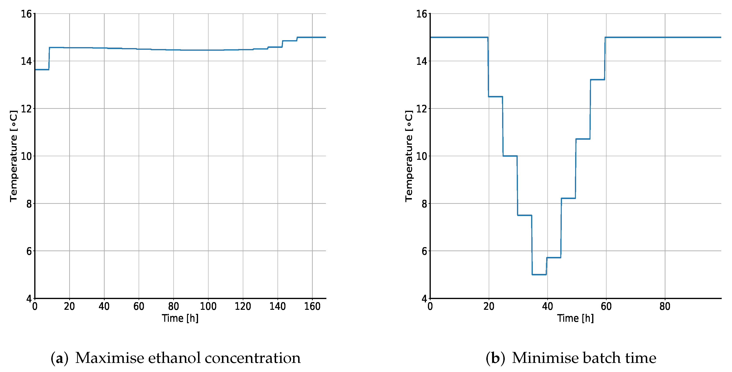
The fermentation model described in Section 2.1 is optimised for two objectives: (i) maximising ethanol production, and (ii) minimising batch time. A constraint on minimum ethanol concentration is imposed. The minimum concentration at the end of the batch is set to 25 g/L. Similarly, an end time constraint on the suspended active cells is also imposed. The maximum concentration of active cells should be less than 0.5 g/L. The two major quality constraints imposed are on the concentrations of diacetyl and ethyl acetate. The maximum concentration of these by-products should be less than 0.2 ppm and 2 ppm, respectively [11,21]. Without accounting for the uncertainty on any of the parameters, the optimised temperature trajectories are depicted in Figure 1a,b.
When maximising the ethanol concentration at the end of the batch, the wort is immediately heated to a relatively high temperature to accelerate the conversion of latent cells to active cells and to enhance the growth of these active cells. The temperature profile stays relatively constant to boost the production of ethanol. This also enhances byproduct formation. The temperature is optimised such that the concentration of ethyl acetate does not exceed 2 ppm. As there is no limit on the batch time, the fermentation continues until all the active yeast cells are consumed. A maximum ethanol concentration of 60.24 g/L is reached in 168 h.
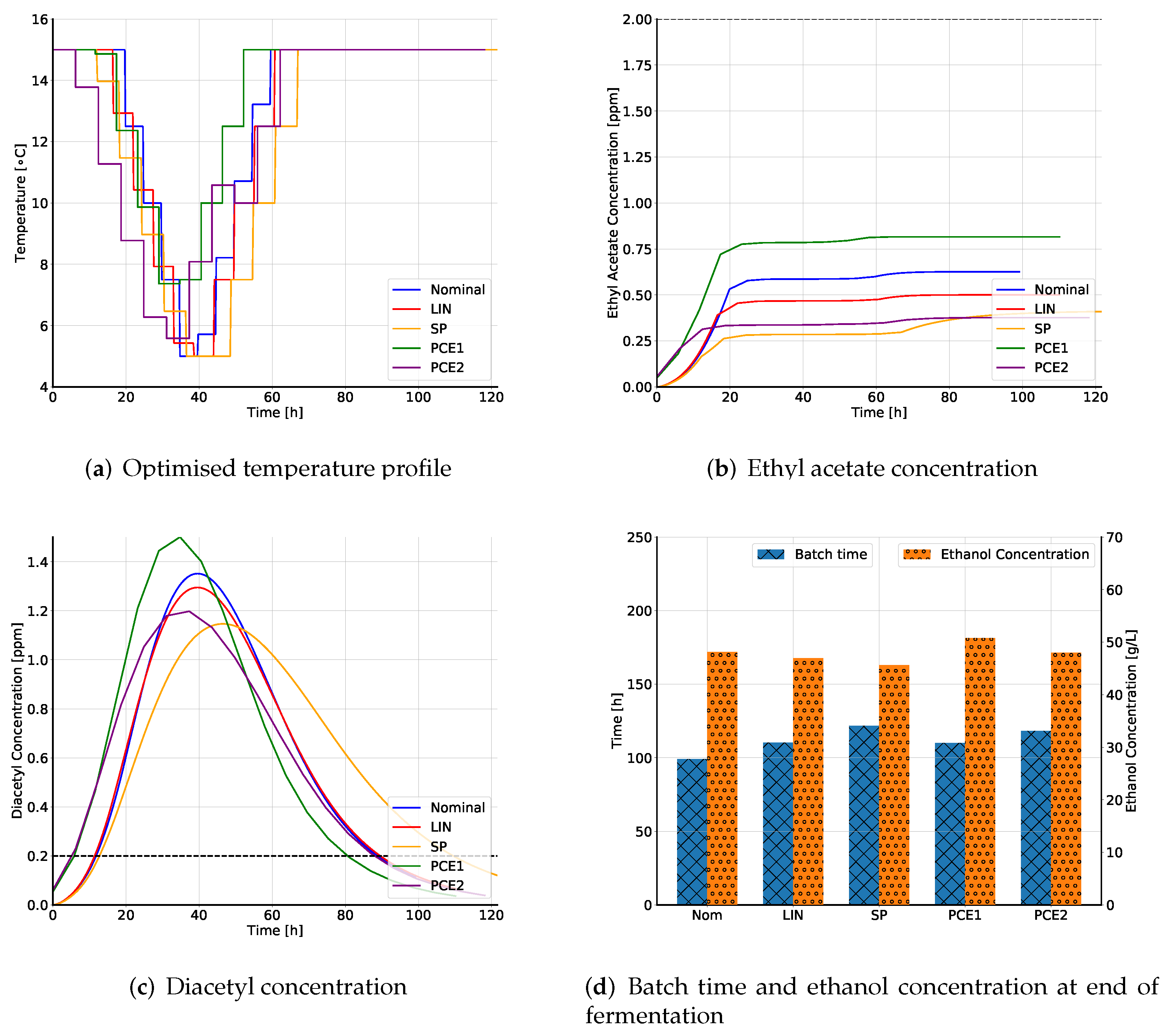
When minimising the batch time, the wort is first heated at the maximum possible temperature (15 °C) to accelerate the the conversion to and the growth of active yeast cells. However, this also accelerates the production of ethyl acetate. Thus after some time, the wort is cooled too rapidly. The cooling occurs in steps because the consecutive temperature jumps are constrained to 2.5 °C/h. This slows down the byproduct formation; however, the ethanol production continues. The evolution of the concentration profiles is depicted in Figure 2b. Towards the end of the batch, the temperature increases again rapidly so as to ensure the active cells are killed and the concentration of yeast cells is below the threshold of 0.5 g/L. The batch stops as soon as this threshold limit is reached. The ethanol concentration achieved is 48.11 g/L in 100 h.

3.1. Influence of Uncertainty

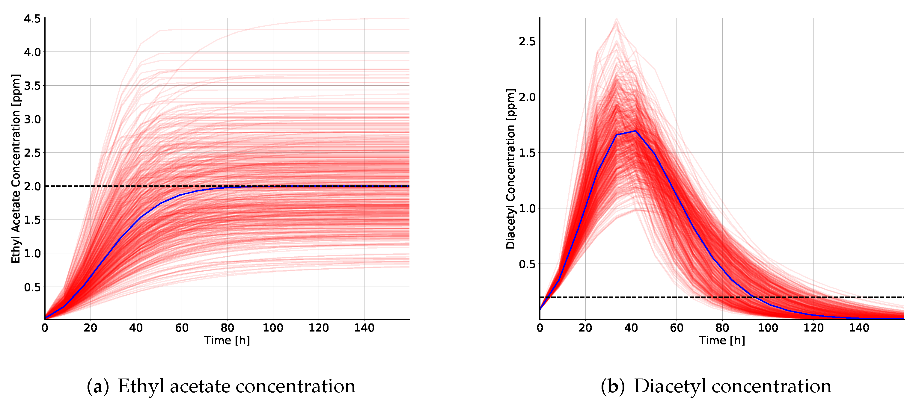
The fermentation model used contains 18 parameters, each of which are determined experimentally. However, considering the uncertainty on each parameter would lead to a very large optimisation problem which would be numerically infeasible. Thus, based on a sensitivity analysis, four parameters which have the most influence on the states of interest (quality parameters) are considered. These are as follows: the maximum growth rate ( μ X , 0 ), yeast death rate ( μ DT ), maximum sugar consumption rate ( μ S , 0 ), and ethyl acetate production ( Y EA ). The only quality parameters considered are the byproducts and the ethanol concentration. Under in silico uncertainty, Figure 3 shows the trajectories of 500 Monte Carlo simulations with the optimal temperature profile obtained for maximising ethanol concentration. The diacetyl concentrations are always below the threshold, while the ethyl acetate concentrations show a large variation and large constraint violation. In total, 50.4% of Monte Carlo simulations violated the ethyl acetate constraint. This exemplifies the need to incorporate the uncertainty into any optimisation study.

3.2. Optimisation under Uncertainty

The uncertainty is incorporated in the optimisation study using the three approaches described earlier. For polynomial chaos expansion, two polynomial orders are used: first order and second order. As the parameter uncertainty is assumed to be Gaussian, Hermite polynomials are used. A desired confidence interval for the constraints is set according to the quantiles of a normal distribution. The backoff parameters used in this study are reported in Table 3. The optimised control profiles are then tested via a Monte Carlo simulation with randomly generated parameter values.

3.2.1. Maximising Ethanol

Figure 4 depicts the results obtained by all the three methods for 95% confidence on the constraint violation. Although concentration of ethanol obtained at the end of the fermentation is similar (slightly lower) to the nominal case, the concentration trajectories of ethyl acetate and diacetyl show differences in the optimised results. Amongst the methods, PCE2 gives the most conservative solution while PCE1 and LIN operate much closer to the concentration bound. This variation is attributed to the approximation of the variance of the concentration values.
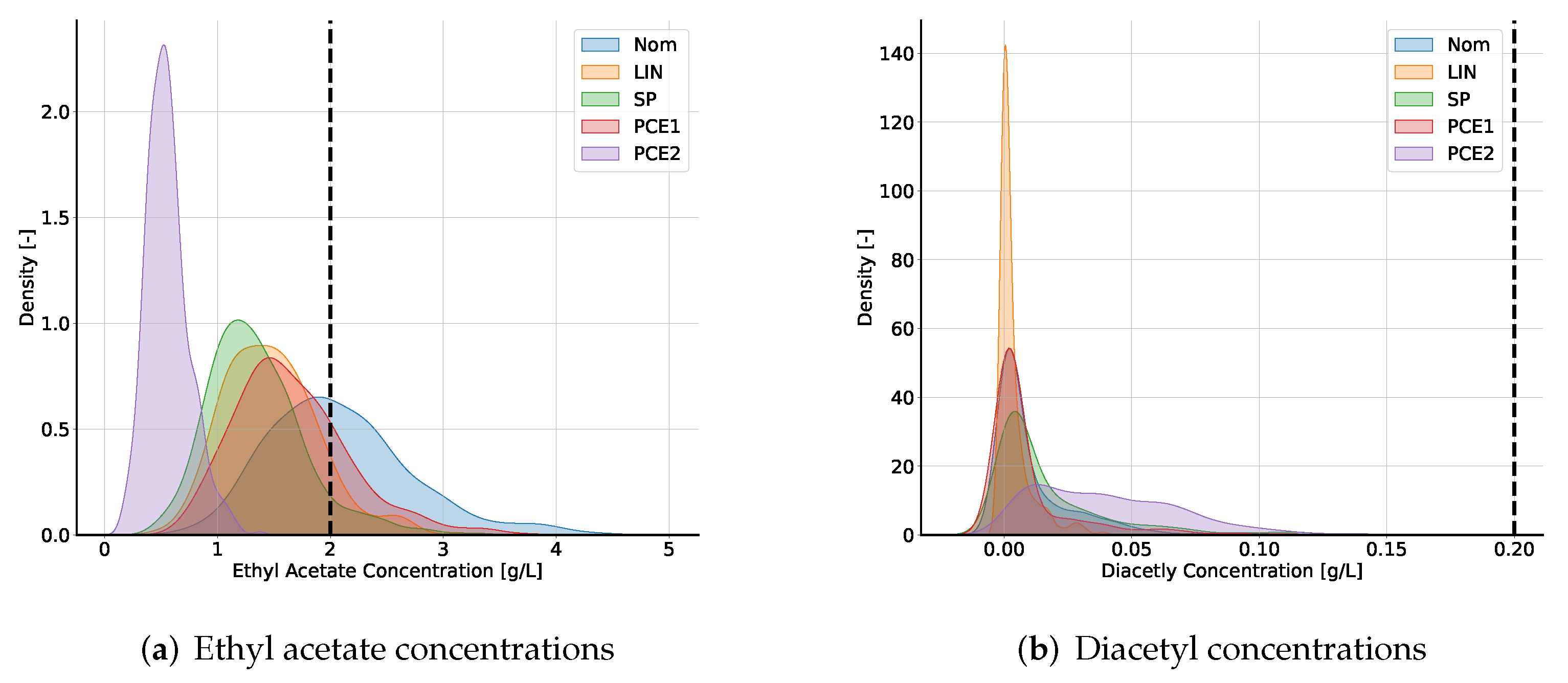
It is impossible to judge a priori which approach provides the best approximation. Thus, the results obtained are assessed using a Monte Carlo simulation. The result with lowest percentage of constraint violation is preferred. The constraint violation as a percentage of the total simulation is reported in Table 4. All methods lead to lower constraint violations than the nominal case. However, second-order polynomial chaos seems to perform the best. The probability densities of the two constraints via the trajectories optimised using all methods are depicted in Figure 5. The majority of constraint violations are caused due to overproduction of ethyl acetate. This is expected from the process dynamics. As concentration evolution of both ethanol and ethyl acetate is described by similar mathematical expressions, maximising ethanol boosts the production of ethyl acetate. However, the conversion/inhibition factors and the production rates differ and are influenced by the temperature differently.

3.2.2. Minimising Batch Time

Figure 6 depicts the results obtained by all the three methods for 95% confidence on the constraint violation. It is seen that all the methods result in longer fermentation batches than the nominal case. As is the case with maximising ethanol, PCE2 and SP give the most conservative solutions while PCE1 and LIN result in fermentation times similar to the nominal case.
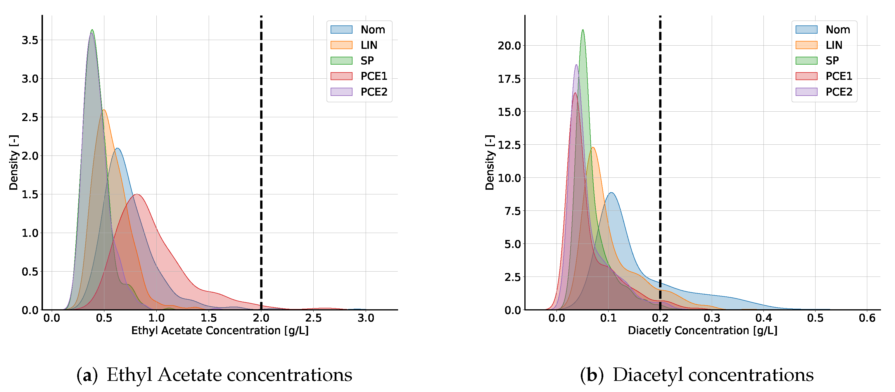
The constraint violation percentage is reported in Table 5. All the robustification approaches lead to a significant reduction in constraint violation. Again, the sigma points approach and PCE2 perform the best in terms of constraint violation. From the concentration density plots (Figure 7) for ethyl acetate and diacetyl, it is observed that when the objective is to minimise batch time, the majority of constraint violations are caused due to excess diacetyl concentration. For the case of maximising ethanol, the constraint violations are caused due to excess ethyl acetate. This can be explained by the dynamics of the process. If the fermentation is allowed to proceed uninterrupted, diacetyl decomposes into a variety of other products. As minimising the batch time essentially interrupts the fermentation, it influences the diacetyl decomposition.

3.2.3. Comparison of Robustification Approaches

For both objectives, the sigma points approach and PCE2 approach perform best in terms of constraint violation. The two first-order methods, linearisation and PCE1, both lead to relatively high constraint violation percentages. As both these methods rely on local linear approximations of a nonlinear model, these methods can be expected to perform poorly when the underlying process model is very nonlinear. However, due to the simplicity of implementation, linearisation is often used despite the poor performance. In the case of maximising ethanol, linearisation performs surprisingly well. This can be explained by the optimised profile. The optimised profile consistently hovers around 14 °C and does not induce any abrupt changes to the process dynamics, leading to a smooth evolution of concentration profiles. In such cases, linearisation is known to perform well. However, when an optimised profile excites the nonlinearity in the model by a big jump (as is the case in minimising time), linearisation over(or under)estimates the variances drastically. This is corroborated by a comparison of the estimated variances of the concentrations with the variance obtained from Monte Carlo simulations reported in Table 6. For maximising ethanol, the variance is estimated with good accuracy, while for minimising batch time, the accuracy reduces. This is consistent with the results of Bhonsale et al. [35], which demonstrate the failure of linearisation when a step change in input is applied to the process exciting its nonlinear dynamics.
A polynomial chaos expansion is fundamentally a reduced-order model of the original process model. In PCE1, the expansion is truncated after the first-order terms making the model linear. The weak performance of PCE1 can be attributed to the local nonlinearity of the fermentation model, which makes the variance approximation poor. Adding a second-order term in PCE2 significantly improves the variance approximation and subsequently the performance of the optimisation under uncertainty.

3.2.4. Effect of Backoff Parameter

As mentioned earlier, the backoff parameter is based on the quantiles of the output distribution. As expected, increasing the value of the back-off parameter (i.e., constraint violations tolerated) leads to a reduction in the percentage of constraint violations for all the methods. This comes at the cost of a more conservation solution. For all methods, an increase in backoff parameter leads to a reduction in the maximum ethanol concentration obtained and longer batch times when the batch time is minimised. It should be noted that in all cases, the tolerances set for the constraint violation are not met. For example, a backoff parameter of 1.65 corresponds to 5% tolerance for constraint violation. However, PCE2, which performs the best for both objectives, still leads to 6.7% and 8.2% violations for maximising ethanol and minimising batch time objectives, respectively. This is because the backoff parameter is based on the quantiles of a normal distribution. It is evident from Figure 5 and Figure 7 that the model output does not follow a Gaussian distribution. Hence, the quantiles used do not exactly correspond to the tolerances. As only two moments, the expectation and the variance, can be obtained from either of the three methods, information on the distribution is impossible to obtain without Monte Carlo simulations. Nevertheless, the reduction in constraint violations with increasing backoff parameters under the assumption of Gaussianity is still significant.

4. Conclusions

Dynamic optimisation has tremendous potential to improve fermentation operation. However, models used in optimisation are inherently uncertain due to their estimation from experimental (noisy) data. It has been shown that if the parametric uncertainty is not included in the optimisation, the state constraints can be violated. Hence, to avoid bad fermentation batches it is necessary to include the uncertainty information available in the optimisation framework.
In this study, a beer fermentation process was optimised while accounting for parametric uncertainty using three techniques. The results obtained with the three techniques were compared for different backoff parameter values. Two objectives, maximising the ethanol concentration and minimising the fermentation time, were considered. While all the methods led to a significant improvement in constraint violation when compared to the nominal case, second-order PCE performed the best. The main advantage of the PCE approach is that no assumption on the distribution of uncertain parameters needs to be made. For independent parameters with certain distributions, the polynomials involved in the PCE can be obtained through the Wiener–Askey scheme [37]. If the parameters are not independent, or do not follow a distribution from the Wiener–Askey scheme, the polynomials can be obtained by utilising the statistical moments and Gram–Schmidt orthogonalisation. However, PCE is computationally expensive as it leads to a significantly bigger optimisation problem. The sigma point approach leads to a smaller optimisation problem while still performing well. However, the direct application of the sigma point approach is limited to parameters with symmetric unimodal distributions. For asymmetric distributions, transformation functions need to be utilised to implement the sigma point approach [49]. Linearisation performs the worst amongst the three approaches. This is expected due to the nonlinearity of the process. However, when the objective is to maximise ethanol linearisation, it performs similarly to the sigma point approach. The study has also emphasised the need for appropriate selection of the backoff parameter.

Author Contributions

Conceptualisation, S.B.; methodology, S.B. and J.V.I.; software, S.B. and W.M.; validation, S.B., W.M., and J.V.I.; formal analysis, W.M. and S.B.; investigation, W.M.; resources, J.V.I.; writing—original draft preparation, S.B.; writing—review and editing, S.B., W.M., and J.V.I.; visualisation, S.B. and W.M.; supervision, S.B. and J.V.I.; project administration, J.V.I.; funding acquisition, S.B. and J.V.I. All authors have read and agreed to the published version of the manuscript.

Funding

This work was supported by KU Leuven Center-of-Excellence Optimization in Engineering (OPTEC), projects G086318N and G0B4121N of the Fund for Scientific Research Flanders (FWO), the European Commission within the framework of the Erasmus+ FOOD4S Programme (Erasmus Mundus Joint Master Degree in Food Systems Engineering, Technology and Business 619864-EPP-1-2020-1-BE-EPPKA1-JMD-MOB) and by the European Union’s Horizon 2020 Research and Innovation programme under the Marie Skłodowska-Curie Grant Agreement N956126 (E-MUSE Complex microbial Ecosystems MUltiScale modElling) and 813329 (PROTECT Predictive mOdelling Tools to evaluate the Effects of Climate change on food safeTy and spoilage).

Institutional Review Board Statement

Not applicable.

Informed Consent Statement

Not applicable.

Conflicts of Interest

The authors declare no conflict of interest.

Abbreviations

The following abbreviations are used in this manuscript:
LINLinearisation
MCMonte Carlo
NLPNon-linear programme
NomNominal
PCEPolynomial chaos expansion
SPSigma point

References

  1. Anderson, K.; Meloni, G.; Swinnen, J. Global Alcohol Markets: Evolving Consumption Patterns, Regulations, and Industrial Organizations. Annu. Rev. Resour. Econ. 2018, 10, 105–132. [Google Scholar] [CrossRef]
  2. Nelson, M. The Barbarian’s Beverage: A History of Beer in Ancient Europe; Routledge: London, UK, 2005. [Google Scholar]
  3. Kirin Beer University. Global Beer Consumption by Country in 2019. 2020. Available online: https://www.kirinholdings.com/en/newsroom/release/2020/1229_01.pdf (accessed on 12 November 2021).
  4. The Brewers of Europe. The Contribution Made by Beer to the European Economy. 2020. Available online: https://brewersofeurope.org/uploads/mycms-files/documents/publications/2020/contribution-made-by-beer-to-EU-economy-2020.pdf (accessed on 12 November 2021).
  5. Belgian Brewers. Annual Report. 2019. Available online: http://www.belgianbrewers.be/en/economy/article/annual-report (accessed on 12 November 2021).
  6. UNESCO. Decision of the Intergovernmental Committee: 11.COM 10.B.5. 2016. Available online: https://ich.unesco.org/en/decisions/11.COM/10.B.5 (accessed on 12 November 2021).
  7. Ministerie Van Economische Zaken. Volksgezondheid en Leefmilieu. In Economische Zaken: Koninklijk Besluit Betreffende Bier. 1993. Available online: http://www.ejustice.just.fgov.be/cgi_loi/change_lg.pl?language=nl&la=N&cn=1993033131&table_name=wet (accessed on 12 November 2021).
  8. Amerine, M.; Pangborn, R.; Roessler, E. Principles of Sensory Evaluation of Food; Academic Press: New York, NY, USA, 1965. [Google Scholar]
  9. Trueba, P.B. Beer Flavour Instability: Unravelling Formation and/or Release of Staling Aldehydes. Ph.D. Thesis, Arenberg Doctoral School, KU Leuven, Leuven, Belgium, 2020. [Google Scholar]
  10. Kobayashi, M.; Shimizu, H.; Shioya, S. Beer Volatile Compounds and Their Application to Low-Malt Beer Fermentation. J. Biosci. Bioeng. 2008, 106, 317–323. [Google Scholar] [CrossRef] [PubMed] [Green Version]
  11. Humia, B.V.; Santos, K.S.; Barbosa, A.M.; Sawata, M.; da Costa Mendonça, M.; Padilha, F.F. Beer Molecules and Its Sensory and Biological Properties: A Review. Molecules 2019, 24, 1568. [Google Scholar] [CrossRef] [PubMed] [Green Version]
  12. Pires, E.J.; Teixeira, J.A.; Brányik, T.; Vicente, A.A. Yeast: The soul of beer’s aroma—A review of flavour-active esters and higher alcohols produced by the brewing yeast. Appl. Microbiol. Biotechnol. 2014, 98, 1937–1949. [Google Scholar] [CrossRef] [Green Version]
  13. Verstrepen, K.J.; Derdelinckx, G.; Dufour, J.P.; Winderickx, J.; Thevelein, J.M.; Pretorius, I.S.; Delvaux, F.R. Flavor-active esters: Adding fruitiness to beer. J. Biosci. Bioeng. 2003, 96, 110–118. [Google Scholar] [CrossRef]
  14. Rodman, A.D.; Gerogiorgis, D.I. Multi-objective process optimisation of beer fermentation via dynamic simulation. Food Bioprod. Process. 2016, 100, 255–274. [Google Scholar] [CrossRef] [Green Version]
  15. Briggs, D.E. Brewing: Science and Practice; CRC Press Woodhead Pub: Cambridge, UK, 2004. [Google Scholar]
  16. Carrillo-Ureta, G.; Roberts, P.; Becerra, V. Genetic algorithms for optimal control of beer fermentation. In Proceedings of the 2001 IEEE International Symposium on Intelligent Control (ISIC ’01) (Cat. No.01CH37206), Mexico City, Mexico, 5–7 September 2001. [Google Scholar] [CrossRef]
  17. Xiao, J.; Zhou, Z.; Zhang, G. Ant colony system algorithm for the optimization of beer fermentation control. J. Zhejiang Uni. Sci. A 2004, 5, 1597–1603. [Google Scholar] [CrossRef] [PubMed]
  18. Rodman, A.D.; Gerogiorgis, D.I. Dynamic optimization of beer fermentation: Sensitivity analysis of attainable performance vs. product flavour constraints. Comput. Chem. Eng. 2017, 106, 582–595. [Google Scholar] [CrossRef]
  19. Bosse, T.; Griewank, A. Optimal control of beer fermentation processes with Lipschitz-constraint on the control. J. Inst. Brew. 2014, 120, 444–458. [Google Scholar] [CrossRef]
  20. Andrés-Toro, B.; Girón-Sierra, J.M.; Fernández-Blanco, P.; López-Orozco, J.; Besada-Portas, E. Multiobjective optimization and multivariable control of the beer fermentation process with the use of evolutionary algorithms. J. Zhejiang Univ. Sci. 2004, 5, 378–389. [Google Scholar] [CrossRef]
  21. Rodman, A.D.; Fraga, E.S.; Gerogiorgis, D. On the application of a nature-inspired stochastic evolutionary algorithm to constrained multi-objective beer fermentation optimisation. Comput. Chem. Eng. 2018, 108, 448–459. [Google Scholar] [CrossRef] [Green Version]
  22. Vanderhaegen, B.; Neven, H.; Verachtert, H.; Derdelinckx, G. The chemistry of beer aging—A critical review. Food Chem. 2006, 95, 357–381. [Google Scholar] [CrossRef]
  23. De Andrés-Toro, B.; Girón-Sierra, J.; López-Orozco, J.; Fernández-Conde, C.; Peinado, J.; Garcia-Ochoa, F. A kinetic model for beer production under industrial operational conditions. Math. Comput. Simul. 1998, 48, 65–74. [Google Scholar] [CrossRef]
  24. Gee, D.A.; Ramirez, W.F. Optimal temperature control for batch beer fermentation. Biotechnol. Bioeng. 1988, 31, 224–234. [Google Scholar] [CrossRef] [PubMed]
  25. Ramirez, W.F.; Maciejowski, J. Optimal Beer Fermentation. J. Inst. Brew. 2007, 113, 325–333. [Google Scholar] [CrossRef] [Green Version]
  26. Trelea, I.C.; Titica, M.; Landaud, S.; Latrille, E.; Corrieu, G.; Cheruy, A. Predictive modelling of brewing fermentation: From knowledge-based to black-box models. Math. Comput. Simul. 2001, 56, 405–424. [Google Scholar] [CrossRef]
  27. Houska, B.; Logist, F.; Van Impe, J.; Diehl, M. Robust optimization of nonlinear dynamic systems with application to a jacketed tubular reactor. J. Process Control 2012, 22, 1152–1160. [Google Scholar] [CrossRef]
  28. Srinivasan, B.; Bonvin, D.; Visser, E.; Palanki, S. Dynamic optimization of batch processes. Comput. Chem. Eng. 2003, 27, 27–44. [Google Scholar] [CrossRef]
  29. Nimmegeers, P.; Telen, D.; Logist, F.; Van Impe, J. Dynamic optimization of biological networks under parametric uncertainty. BMC Syst. Biol. 2016, 10. [Google Scholar] [CrossRef] [Green Version]
  30. Mesbah, A.; Streif, S.; Findeisen, R.; Braatz, R.D. Stochastic nonlinear model predictive control with probabilistic constraints. In Proceedings of the 2014 American Control Conference, Portland, OR, USA, 4–6 June 2014. [Google Scholar] [CrossRef]
  31. Mesbah, A.; Streif, S. A Probabilistic Approach to Robust Optimal Experiment Design with Chance Constraints. IFAC-PapersOnLine 2015, 48, 100–105. [Google Scholar] [CrossRef]
  32. Telen, D.; Vallerio, M.; Cabianca, L.; Houska, B.; Van Impe, J.; Logist, F. Approximate robust optimization of nonlinear systems under parametric uncertainty and process noise. J. Process Control 2015, 33, 140–154. [Google Scholar] [CrossRef] [Green Version]
  33. Vallerio, M.; Telen, D.; Cabianca, L.; Manenti, F.; Van Impe, J.; Logist, F. Robust multi-objective dynamic optimization of chemical processes using the Sigma Point method. Chem. Eng. Sci. 2016, 140, 201–216. [Google Scholar] [CrossRef]
  34. Akkermans, S.; Nimmegeers, P.; Van Impe, J.F. A tutorial on uncertainty propagation techniques for predictive microbiology models: A critical analysis of state-of-the-art techniques. Int. J. Food Microbiol. 2018, 282, 1–8. [Google Scholar] [CrossRef] [PubMed]
  35. Bhonsale, S.; Telen, D.; Stokbroekx, B.; Van Impe, J. An Analysis of Uncertainty Propagation Methods Applied to Breakage Population Balance. Processes 2018, 6, 255. [Google Scholar] [CrossRef] [Green Version]
  36. Julier, S.; Uhlmann, J.K. A General Method for Approximating Nonlinear Transformations of Probability Distributions; Technical Report; Robotics Research Group, Department of Engineering Science, University of Oxford: Oxford, UK, 1996. [Google Scholar]
  37. Xiu, D.; Karniadakis, G. The Wiener–Askey polynomial chaos for stochastic differential equations. SIAM J. Sci. Comput. 2002, 24, 619–644. [Google Scholar] [CrossRef]
  38. Bhonsale, S.; Muñoz López, C.A.; Van Impe, J. Global Sensitivity Analysis of a Spray Drying Process. Processes 2019, 7, 562. [Google Scholar] [CrossRef] [Green Version]
  39. Yang, S.; Xiong, F.; Wang, F. Polynomial Chaos Expansion for Probabilistic Uncertainty Propagation. In Uncertainty Quantification and Model Calibration; InTech Open: London, UK, 2017. [Google Scholar] [CrossRef] [Green Version]
  40. Navarro, M.; Witteveen, J.; Blom, J. Polynomial Chaos Expansion for general multivariate distributions with correlated variables. arXiv 2014, arXiv:1406.5483. [Google Scholar]
  41. Paulson, J.A.; Buehler, E.A.; Mesbah, A. Arbitrary Polynomial Chaos for Uncertainty Propagation of Correlated Random Variables in Dynamic Systems. IFAC-PapersOnLine 2017, 50, 3548–3553. [Google Scholar] [CrossRef]
  42. Ghanem, R.; Spanos, P. Stochastic Finite Elements—A Spectral Approach; Springer: Berlin/Heidelberg, Germany, 1991. [Google Scholar]
  43. Debusschere, B.; Najm, H.; Pébay, P.; Knio, O.; Ghanem, R.; Maitre, O.L. Numerical challenges in the use of polynomial chaos representations for stochastic processes. SIAM J. Sci. Comput. 2004, 26, 698–719. [Google Scholar] [CrossRef]
  44. Tatang, M.; Pan, W.; Prinn, R.; McRae, G. An efficient method for parametric uncertainty analysis of numerical geophysical models. J. Geophys. Res. Atmos. 1997, 102, 21925–21932. [Google Scholar] [CrossRef]
  45. Biegler, L.T. An overview of simultaneous strategies for dynamic optimization. Chem. Eng. Process. Process Intensif. 2007, 46, 1043–1053. [Google Scholar] [CrossRef]
  46. Wächter, A.; Biegler, L.T. On the implementation of an interior-point filter line-search algorithm for large-scale nonlinear programming. Math. Program. 2005, 106, 25–57. [Google Scholar] [CrossRef]
  47. Bhonsale, S.; Telen, D.; Vercammen, D.; Vallerio, M.; Hufkens, J.; Nimmegeers, P.; Logist, F.; Van Impe, J. Pomodoro: A Novel Toolkit for Dynamic (MultiObjective) Optimization, and Model Based Control and Estimation. IFAC-PapersOnLine 2018, 51, 719–724. [Google Scholar] [CrossRef]
  48. Andersson, J.A.E.; Gillis, J.; Horn, G.; Rawlings, J.B.; Diehl, M. CasADi—A software framework for nonlinear optimization and optimal control. Mathe. Program. Comput. 2019, 11, 1–36. [Google Scholar] [CrossRef]
  49. Neumann, T.; Dutschk, B.; Schenkendorf, R. Analyzing uncertainties in model response using the point estimate method: Applications from railway asset management. Proc. Inst. Mech. Eng. Part O J. Risk Reliab. 2019, 233, 761–774. [Google Scholar] [CrossRef]
Figure 1. Optimised temperature profiles for the nominal case with two different objectives: maximising ethanol concentration and minimising batch time.
Fermentation 07 00285 g001
Figure 2. Concentration profiles of ethanol and the two byproducts for the nominal case with two different objectives: maximising ethanol concentration and minimising batch time. The byproducts are represented on the left y-axis and ethanol on the right y-axis. The horizontal lines depict the constraints on the byproducts.
Fermentation 07 00285 g002
Figure 3. Concentration profiles of the two byproducts for the nominal case with maximising ethanol concentration as the objective, and minimising batch time. The blue trajectory represents the simulation with the nominal parameter value and the red trajectories depict the Monte Carlo simulations. The horizontal dashed lines depict the constraints on the byproducts.
Fermentation 07 00285 g003
Figure 4. Optimisation results for maximising ethanol with all three methods and α = 1.65 . The concentration trajectories depicted were obtained by applying the optimised temperature trajectory to the model with nominal parameters.
Fermentation 07 00285 g004
Figure 5. Density plots for concentrations of ethyl acetate and diacetyl based on Monte Carlo simulations for optimal trajectory obtained with maximising ethanol. The vertical dashed line depicts the concentration threshold.
Fermentation 07 00285 g005
Figure 6. Optimisation results for minimising time with all three methods and α = 1.65 . The concentration trajectories depicted were obtained by applying the optimised temperature trajectory to the model with nominal parameters.
Fermentation 07 00285 g006
Figure 7. Density plots for concentrations of ethyl acetate and diacetyl based on Monte Carlo simulations for optimal trajectory obtained with minimising time. The vertical dashed line depicts the concentration threshold.
Fermentation 07 00285 g007
Table 1. Rate expressions used in the dynamic model.
ComponentRate Expression
Settling of dead cells μ SD = 0.5 μ SD , 0 C S , 0 0.5 C S , 0 + C eth
Biomass growth μ X = μ X , 0 C S k s + C S
Sugar consumption μ S = μ S , 0 C S k s + C S
Ethanol formation μ X = μ eth , 0 C S k s + C S
Ethanol inhibition f = 1 C eth 0.5 C S , 0
Diacetyl formation μ DY = 1.2762 × 10 4
Diacetyl conversion μ AB = 1.13864 × 10 3
Table 2. Parameters in the Arrhenius-type rate constants.
Description A i B i
Maximum settling rate of dead cells, μ SD , 0 33.82−10,033.28
Maximum growth rate, μ X , 0 108.31−31,934.09
Maximum sugar consumption rate, μ S , 0 41.9211,654.64
Maximum ethanol production rate, μ eth , 0 3.27−12,667.24
Yeast death rate, μ DT 130.16−38,313.00
Yeast activation rate, μ SD , 0 30.72−9501.54
Affinity constant, k s −119.6334,203.95
Ethyl acetate production, Y EA 89.92−26.589
Table 3. Backoff parameter ( α ) values corresponding to the confidence intervals.
Confidence Level90%95%97.50%
Quantile0.10.050.025
α 1.281.651.96
Table 4. Constraint violations obtained from Monte Carlo simulations for the maximising ethanol objective via all the methods and backoff parameter values.
LinearisationSigma PointsPCE 1PCE 2Nominal
α = 1.28 19.6%18.5%35.3%9.5%
α = 1.65 13.6%13.0%27.6%6.7%50.4%
α = 1.96 11.1%9.6%21.6%5.4%
Table 5. Constraint violations obtained from Monte Carlo simulations for the minimising time objective via all the methods and backoff parameter values.
LinearisationSigma PointsPCE 1PCE 2Nominal
α = 1.28 35.5%17.2%37.7%17.2%
α = 1.65 29.3%8.4%20.1%8.2%70.4%
α = 1.96 24.5%4.6%14.4%4.4%
Table 6. Comparison of variances approximated using linearisation with variances approximated by Monte Carlo simulations for α = 1.65 .
VarianceMaximise EthanolMinimise Batch Time
LinearisationMCLinearisationMC
V C EA 1.56 × 10 1 1.79 × 10 1 1.20 × 10 2 1.70 × 10 2
V C DY 5.16 × 10 4 5.38 × 10 4 2.60 × 10 3 1.57 × 10 3
V C eth 1.19 × 10 1 1.42 × 10 1 1.54 × 10 1 2.29 × 10 1
Publisher’s Note: MDPI stays neutral with regard to jurisdictional claims in published maps and institutional affiliations.