Abstract
Recently there has been an increased interest in characterising the rates of alcoholic fermentations. Sigmoidal models have been used to predict changes such as the rate of density decline. In this study, three published sigmoidal models were assessed and fit to industrial fermentation data. The first is the four-parameter logistic model described in the ASBC Yeast-14 method. The second model is a nested form of the four-parameter logistic function, adding an extra parameter, creating the 5-parameter logistic equation., where an additional parameter was added to allow for asymmetry. The final model is a three-parameter logistic equation which describes the change in the Apparent Degree of Fermentation with time. The three models were compared by fitting them to industrial data from Australian and Canadian lagers, American and Scottish ales and Scotch Whisky fermentations. The model fits were then compared to one another with a technique developed by Akaike and a nested F-test. The Akaike information criterion compares the models and accounts for both the goodness of fit, and the number of parameters in the model. Finally, consideration was given to the establishment of prediction bands (that enclose the area that one can be 99% sure contains the true datapoints). Calculation of these bands was “challenging” but successful as the industrial fermentation data was heteroscedastic.
1. Introduction
In recent years, the development of advanced regression software has facilitated the application of logistic regression models to beer and whisky fermentations [1]. If one follows the decline in density of batch fermentations (typically represented as °Plato, °Brix, or specific gravity), in almost every instance, a sigmoidal curve results. On rare occasions where very active yeast is pitched, no lag phase will be observed and only an exponential decline will be noted. However, this behaviour can be modelled with a ‘nested’ version of the logistic model. The four-parameter logistic equation was first applied to Australian lager fermentations [1] and has also been successfully employed to identify Premature Yeast Flocculation (PYF) fermentations by the variation of fermentation parameters when compared to controls [2]. This model forms part of the ASBC Yeast-14 assay [3]. Predictive regression allows brewers to compare the effect of yeasts, malts and other process changes, correlate other fermentation products (such as CO2) and predict final attenuation values. Predictive regression can also provide further insights to fundamental aspects of fermentation including lag time and total fermentation time. While not perfect, this technique helps brewers to better optimize their operations and detect aberrant behaviour. After nearly two decades since the first analysis of the rate of density decline [1], it is appropriate to test the suitability of logistic models to model change in the fermenting medium density. The objective of this study was to comparatively assess the most commonly applied models and techniques on seven large fermentation datasets of varying size collected from brewing, whiskey and laboratory sources.
A linear equation includes predictions that are “linearized” with respect to a single parameter. This includes common equations for a straight line such as exponential curves, and other linear transforms. Non-linear regression is required when there are multiple parameters that describe different aspects of the model, and a transform in the primary parameter does not induce a linear response in the dependent variable. Non-linear models allow users to mathematically describe fermentation rates that increase at the beginning and decline at the end. While more complex than a linear regression which consist of only two adjustable parameters (the slope and intercept) the four-parameter logistic equation describes the sigmoidal shape of the decline in density with respect to time as shown in Equation (1). In the case of non-linear models, the best fits are normally selected by systematic computer adjustment of the parameters of the equation to minimize the residual sum of squares (RSS). A typical plot for this model with respect to time shown in Figure 1. This equation is often termed logistic, or autocatalytic as it describes an exponential increase in fermentation rate, followed by an inflection and a subsequent exponential decrease in the rate of density decline. The application of this non-linear regression model to predict fermentation behaviour allows a more accurate comparison of both industrial and experimental fermentations and has been applied by various authors in the field, for example [4,5].
where Pt is the Apparent Extract (AE—expressed in oPlato at a time ‘t’), M is the inflection point of the curve, or where the rate of extract decline is maximal, Pi is the upper asymptote, Pe is the lower asymptote or AE as time approaches ∞, and B is a function of the slope at M (B = doP/dt at M * e/(Pi − Pe) which describes the maximum rate (gradient).
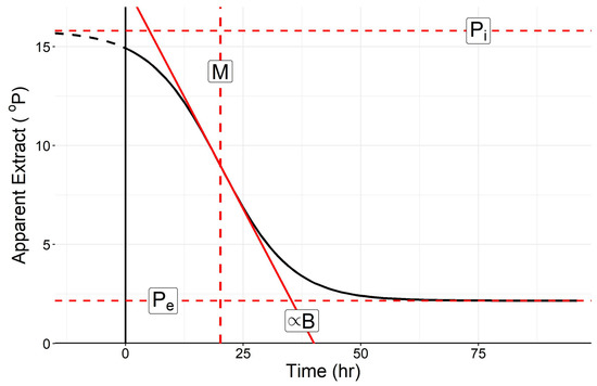
Figure 1.
The shape of a four-parameter logistic equation modeling the decline in density with time for a typical fermentation (modified from Speers et al. [1,3]).
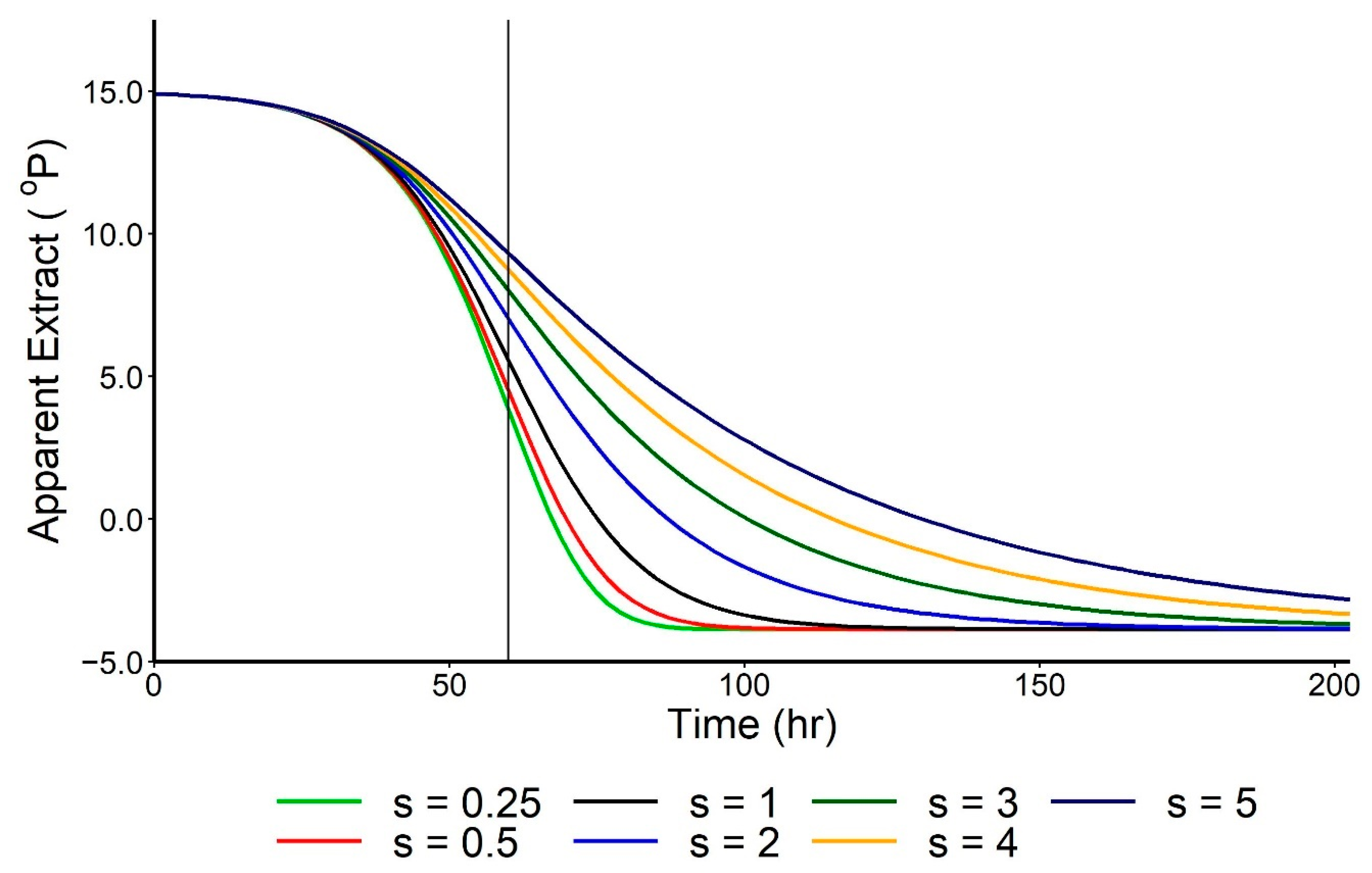
Subsequent to the use of this logistic model in brewing, a five-parameter model first proposed by Richards in 1959 [6] was employed by MacIntosh and Speers to first model the asymmetrical consumption of individual wort sugars [7,8]. This model is known as a “generalised” logistic and can be also applied to consumption curves that are asymmetrical around the inflection point. The additional parameter “s” introduced in this model describes the asymmetric behaviour. When s = 1, this model reverts to the four-parameter logistic. The equation for the model is shown in Equation (2) and Figure 2.
where Pt, Pe, Pi, B, and M are as described previously and s is an adjustable parameter which permits fitting asymmetric attenuation curves such as those demonstrating a substantial lag, or slow finishing attenuation.
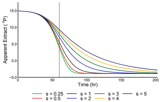
Figure 2.
The generalised shape of a five-parameter logistic equation modeling the decline in density with time for a typical fermentation (showing the effect of ‘s’ parameters ranging from 0.25 to 5).
The third recently reported model [9] is another variant of the logistic model and predicts the change in the density as the Apparent Degree of Fermentation (ADF). Traditionally, ADF is calculated from density measurements of the wort and beer density taken at the beginning and end of the fermentation:
where the Original Extract or ‘OE’ is the starting extract P0 and Pt is the final Apparent Extract (AE), respectively. Normally the Apparent Extract is measured at the cessation of fermentation but can refer to the density of the ferment at any time after the start of the fermentation. Similarly, ADF values can be calculated at any time through the fermentation by use of the Apparent Extract at time t or Pt:
where ADFt is the ADF at any time t or (P0 − Pt)/P0), ADFe is the asymptotic limit and B and M are parameters as described in the logistic model (Equation (1)). Equation (3) effectively takes the form of a three-parameter logistic function. This model relies on the assumption that the final condition forms an asymptote parallel to the x axis. In the case of ADF, the initial condition (equivalent to Pi in the four-parameter model) is assumed to form this asymptote. The difficulty with the use of this method as reported is that the Original Gravity or P0 must be fixed rather than be free to allow the best fit. Practically, P0 is set to the largest density value in the fermentation dataset. This procedure is analogous to assuming or fixing an intercept in linear regression, limiting one’s ability to accurately predict the change in the dependent variable ADFt.
To determine the best fit parameters of a given model to a dataset, optimization software is used to minimize the residual sum of squares (i.e., RSS or error of the model) by adjusting the variables in a systematic fashion. Whilst once an intensive computing technique, various software packages ranging in complexity from Excel to R can now easily determine the best fit of non-linear models to the data. An excellent discussion of this technique is given by Motulsky and Ransnas [10]. When fitting attenuation data, there remains the problem of determining which model best fits the data when the models possess different parameters and shapes. A method developed by statistician Hirotugu Akaike, and termed the “Akaike information criterion” is a common method for comparing models within the field of statistics. This criterion uses various characteristics of the models including parameterisation and transformations to assist with model selection. Calculation of the Akaike information criterion (AICc, ‘c’ for corrected [11]) results in a value that can be used to determine how well the data fits the model. Furthermore, use of the weighted AIC (ω) allows the comparison of models by normalising the AIC scores, with the sum of all assigned score equal to unity. Another method of determining the best model is the F-test, which is appropriate for nested models (those that share parameters). This allows the determination of whether there is statistical evidence of significant difference between models. Through defining whether significant difference exists avoids the model becoming overparameterised, thus, ‘overfitting’ the data to the model. As a result, the statistician can use a combination of both the AIC and F-tests to determine which model best fits the observed fermentation data. Using these metrics allows consideration of both the ability of a chosen model to reduce RSS but also considers the parameterisation of the model, with a view to accept the lowest number of parameters as possible. The determination of the best fit model may not be obvious from simply plotting the observed data. Therefore, it is important that the best model is established when analysing fermentations.
Finally, once an optimal model has been established, it becomes possible to construct prediction bands to delineate the error in the nonlinear regression curves. Prediction bands are useful tools in detecting aberrant fermentations, scheduling and prediction. While it is relatively easy to predict the upper and lower bands when the error is constant with respect to time (homoscedastic), examination of the error with time for real fermentation data often reveals curves that are substantially heteroscedastic. This was first reported in 2003 for the Australian Lager dataset and examination of other datasets also revealed heteroscedastic behaviour. In this study, A method to generate prediction bands was hypothesised using dataset 7 by first calculating the standard deviation at each time and calculating high and low values using a correction for heteroscedasticity as follows:
where X is the mean, SD is the standard deviation and n is the number of datapoints at the selected time. Once calculated, the logistic equation was fit to these high or low values to form prediction bands above and below the fit curve.
X ± 3*SD*(1 + 1/n)0/.5
To meet our objective of assessing models and techniques, we first collected data from industrial brewing, whisky and laboratory sources. We then tested the hypothesis that the four-parameter model was the ‘best’ model to predict the change in density with time by fitting each curve and statistically comparing the results. After the datasets were effectively modeled and compared, we assessed the suitability of Equation (5) to effectively bound the datasets with prediction bands while considering heteroscedastic behaviour.
2. Materials and Methods
A number of datasets were collected from industrial and laboratory fermentations of beer and Scotch whisky from 2003 to 2020 in Australia, Canada, Scotland and the United States as shown in Table 1.

Table 1.
Fermentations monitored.
With the exception of the large laboratory-based Canadian dataset (dataset 7), the fermentations were undertaken at industrial breweries of various sizes. Much of the details of these fermentations are proprietary. However, dataset 1 was obtained from a commercial Scottish ale brewery in 2014. These 40 ale fermentations were hopped at 30 IBU, oxygenated wort and fermented with acid washed yeast [12] at 17 °C with an Original Extract of 10.0 °P. It is noteworthy that dataset 1 was collected at a time when the brewery pitched the yeast cell slurry by volume, not cell count, leading to substantial variation [12]. The second dataset (US Pale Ale) was collected in 2010 and was fermented at 20 °C, with 13.1 °P wort, hopped to ~40 IBU. The next two whisky datasets were pitched in 2019 at 17 °C with a S. cerevisiae distillers’ yeast, free-rising to 33 °C during fermentation. As traditional, the Scotch whisky mashes were un-boiled, un-hopped and underwent no oxygenation [13]. The Australian lager had an Original Extract of 14.1 °P and starting temperature of 10 °C and was fermented in 2001 and subject of the original modelling study [1]. Dataset 7 was a collection of various malted barley fermentations assessed using ASBC Yeast-14 [3].
Each of the three logistic models were fit to all fermentation in each dataset using both prism and “R”. By using Prism software (Prism 8.4.3, GraphPad Software, San Diego, CA, USA, www.graphpad.com) or other statistical software such as R (R-4.0.3, R Foundation for Statistical Computing, Vienna, Austria), one can calculate the lowest ΔAICc to determine the best fit model. The AICc for each model was determined and all models were compared in order to make meaningful comparisons between each level of parameterisation. AICc weights (ω) and p-values resulting from F-tests were computed in R, running the RStudio GUI (V1.3.1093 RStudio Inc., Boston, MA, USA). This was then fed into a decision-making algorithm which statistically determined the model of best fit [13].
Finally, prediction bands were constructed on the largest of datasets to assess the effectiveness of the proposed correction to incorporate heteroscedasticity into prediction bands for the fermentation industries.
3. Results and Discussion
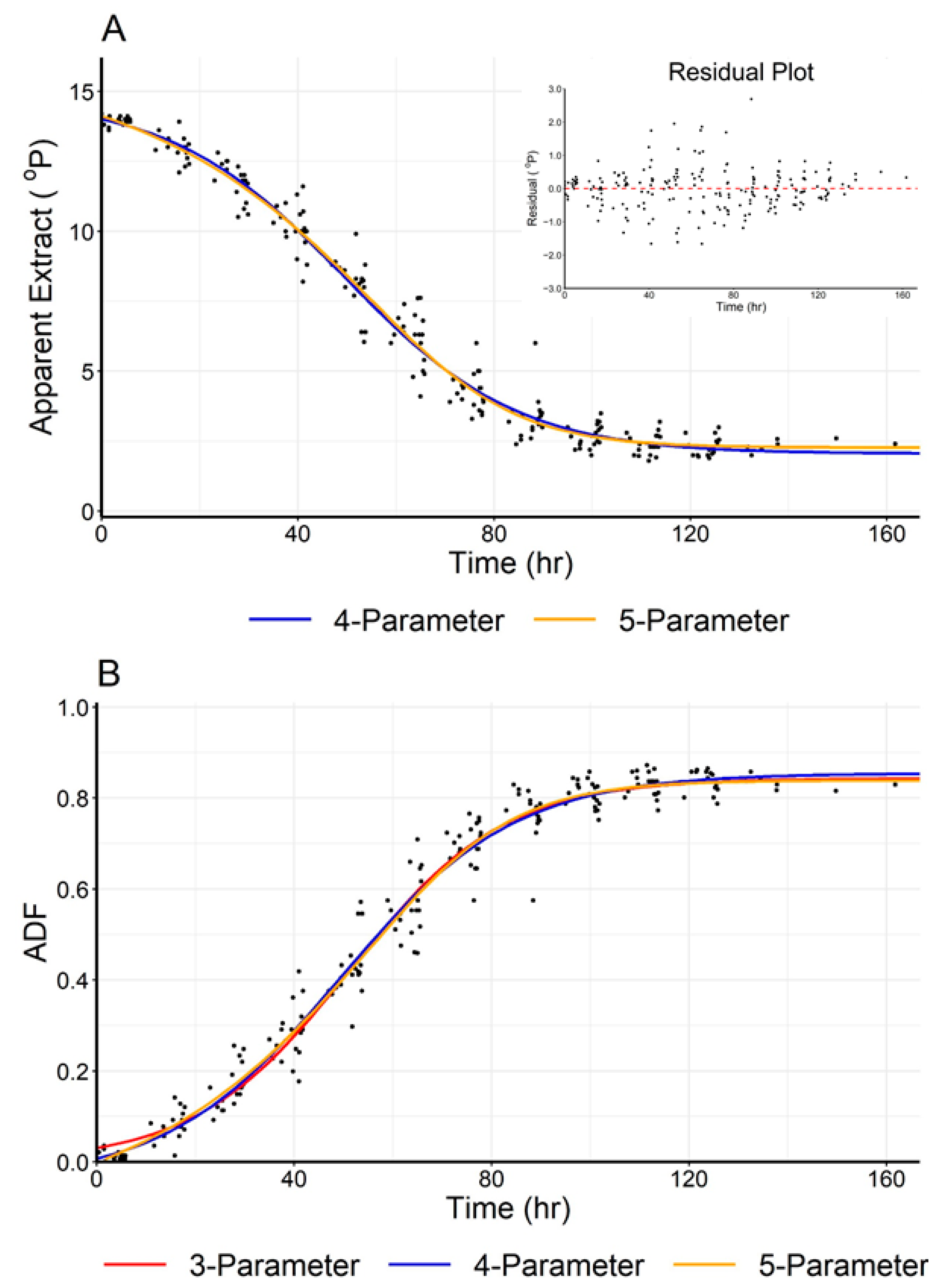
Each model was successfully fit to each dataset, and an example comparison of models is shown in Figure 3, where the three-, four-, and five-parameter models are fit to dataset 5 (Australian Lager). The statistical fit of each model is given in Table 2; and by examination of curve fits and residuals, all three models fit the data well. However, as discussed above, one must fix an OG to calculate the ADFt values.
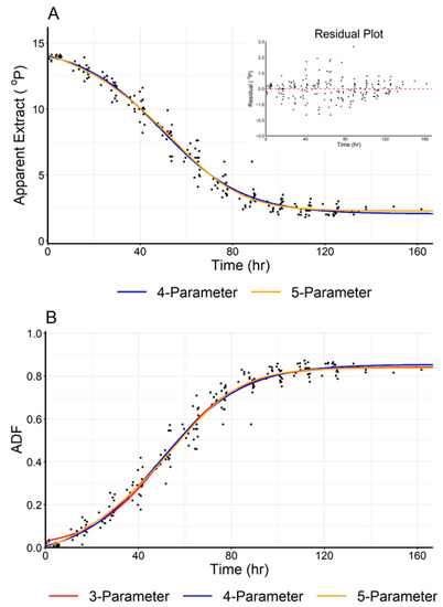
Figure 3.
(A) A visual comparison of the four- and five-parameter models (Equations (1) and (2)) showing the dependence of Apparent Extract with time for fermentation five (Australian lager). The red line is the five-parameter model while the blue line indicates the four-parameter model. The insert shows the heteroscedasticity of the data based on the four-parameter logistic fit. (B) A comparison of the change in the ADFt as predicted by the three- (i.e., ADF), four- and five-parameter models. ADF was calculated by assuming the OE was 14.1 °P to provide a visual comparison of all three models.

Table 2.
Statistical evaluation of the curve fit of the Australian lager fermentation.
Using the best fit results from each dataset, the AICc and F-test were used to compare each model. These statistics are shown in Table 3. No one model was determined to best fit all the datasets. Both the three-parameter and four-parameter models were selected as the optimal model twice, with the five-parameter being selected three times as the best fitting model by the AICc and F-test criteria. There was evidence to suggest that lager fermentations are not modelled well by the ADF function which was noted by the very low AICc weights assigned to these models. This effect, however, may be offset by the influence of the high number of observations. The five-parameter model provided a substantial reduction in RSS when there is a much larger number of datapoints describing the fermentation, which will benefit from the overfitting (i.e., an analysis that corresponds too closely or exactly to a particular set of data) of these plots.

Table 3.
Computation of AICc weights (ω) and p-values resulting from F-tests of all seven fermentation types. The higher parameterised model incurs a significant reduction in error when p < 0.05. Furthermore, the highest ω presents the model which has the most favourable AICc score.
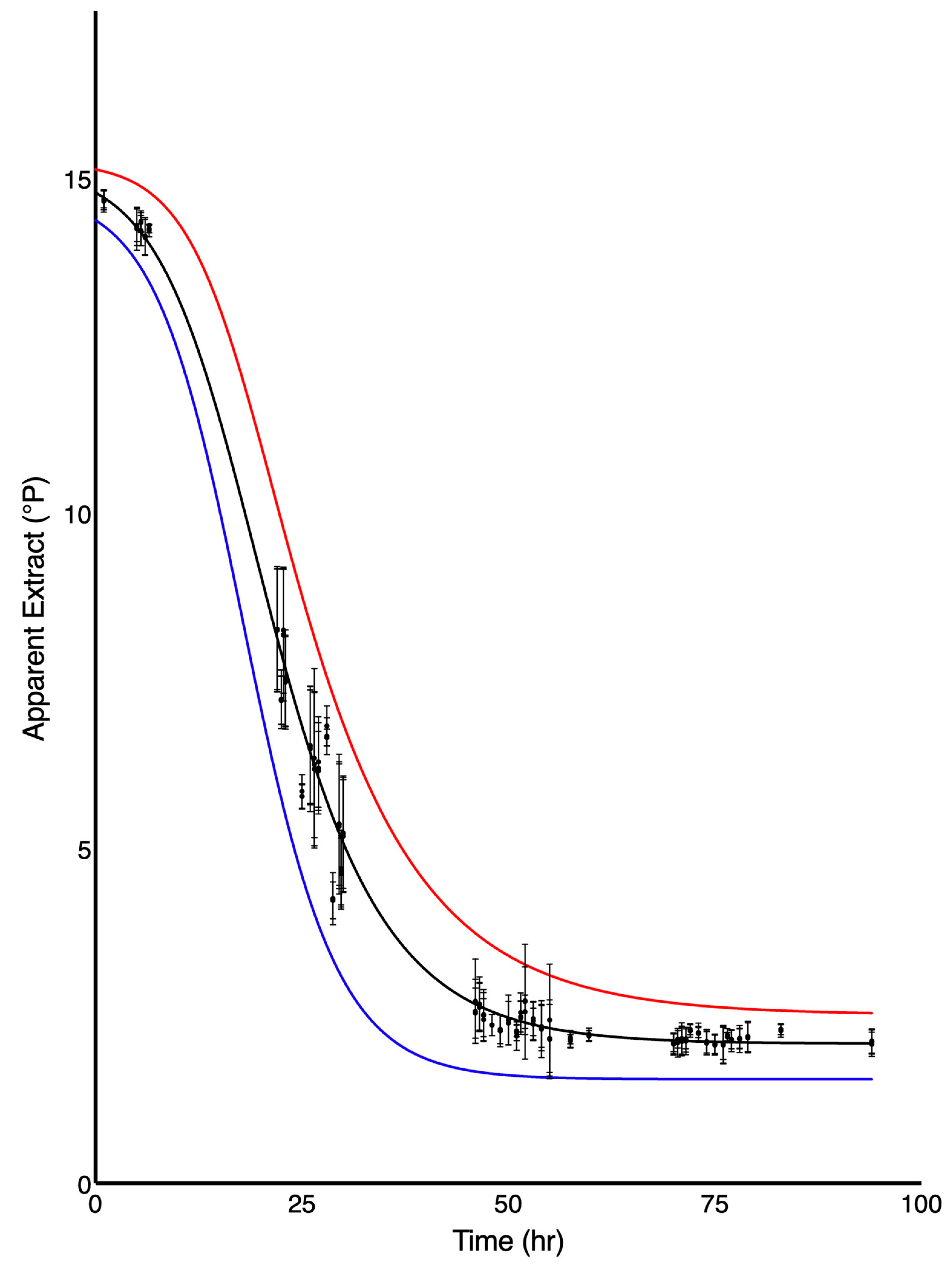
As mentioned above, all the fermentations could be fit with the three-, four- or five-parameter models. The combined fits from the 78 trials in dataset 7 are shown in Figure 4, where the five-parameter model (Equation (2)) was applied. While the initial and final density within this dataset are very similar, there are differences in the rate of fermentation between batches resulting in a large amount of variability during periods of active attenuation. This is typical of all batch fermentations and can be due to small changes in yeast, sugars, temperature, etc. A model with variability that is dependent upon another parameter (in this case time) is evidence of heteroscedasticity. This heteroscedasticity was also found in other datasets (see for example Figure 3) and must be accounted for in the construction of prediction bands. (which bound the area where one would expect 99% of data points to lie). While difficult, realistic calculation of heteroscedastic prediction bands can be made provided the dataset is large enough and contains enough density values at set sampling times of low variability. Prediction bands were constructed for dataset 7 using Equation (5) where 2486 points were available. These bands are shown in Figure 4 which includes the upper and lower 99% prediction bands for this dataset.

Figure 4.
The fit of the five-parameter model to the pooled 78 fermentations of dataset 7. The red and blue lines indicate the prediction band where 99% of the data points could be expected to lie. Points and error bars indicate the mean and standard deviation at each measured time.
Each model presented during this study demonstrates both positive and negative attributes. The three-parameter model, although often produces the most suitable model (Table 3), requires the transformation of observed data to the form of ADF (Equation (3)). This form, although valid, requires an exact measurement of the original extract (OE). As a result, an uncertain OE value can lead to inconsistent or erroneous modelling, especially if the OE is subject to error. Despite this potential area of inconsistency, the three-parameter model is most useful when assumptions about the initial condition can be made. This includes modelling the evolution of CO2 or weight loss during fermentation, both of which will follow a similar logistic pattern. As at the beginning of fermentation this value must equal zero (similarly with ADF), the initial state of the three-parameter model holds true (time = 0, y = 0). When such a condition exists, higher parameterisation, may not involve the addition of another asymptotic value (such as Pi) but instead may incorporate the parameter, s (as is observed in Equation (2)), to account for asymmetry in the observed data.
The five-parameter model provides an asymmetric regression fit. This asymmetrical fermentation profile was exhibited in both lager and whisky fermentations studied. The five-parameter model will be preferentially chosen when the number of observations is high. This is due to the reduction in RSS which must exist in order to support the extra parameter. When s = 1, the model will take the form of the four-parameter regression. As a result, when there is a lack of asymmetry in the model, convergence of this five-parameter regression may not be achieved, causing the model to fail. In this case, the three- or four-parameter model must be considered instead. To reemphasize, with the high number of observations and slight asymmetry, the five-parameter model will be the best applicable model. This is demonstrated by dataset 7 in Table 3.
The four-parameter model offered good all-round support of the modelling of density decline during fermentation, but became inaccurate as the fermentation became asymmetric. Model convergence was achieved most often using this system and no transformation of the dataset was required prior to model fitting.
4. Conclusions
Fermentation modelling provides a useful tool to monitor, track and predict fermentation characteristics within a brewhouse. Model selection has previously indicated that the logistic equation demonstrates good agreement with density decline during fermentation by yeast. Overall, the comparison of the three sigmodal-shaped models leads one to conclude that no one model fits all the datasets best. There was often little difference in the visual fit of the four- and five-parameter models as shown in Figure 3. However, for datasets 3, 5 and 7, close examination of the model fits revealed that the five-parameter model fit was in fact the best fit, when only comparing the reduction in residual sum of squares (RSS). This in turn caused a reduction in the AICc value despite the increase in parameterisation of the model and resulted in a greater AICc weight (ω). Furthermore, analysis of the nested F-test proved that there was significant reduction (p < 0.05) in error when moving from the four-parameter to the five-parameter model. This provided compelling evidence to support the use of the five-parameter model for the fermentation when asymmetry was observed. The five-parameter model tends to provide a better fit as the number of data points increase as it provides increased flexibility. However, in very symmetrical datasets, the three- or four-parameter models may prove superior.
As no one model fit all the data presented and no trends between fermentation type or scale were evident, it was determined that the most effective model for a given system must be determined through the use of empirical evidence. The use of AICc weights was observed to provide a useful method for comparing a variety of models. Furthermore, the nested F-test allowed the determination of whether moving to a higher parameterisation resulted in a significant reduction in error. These tools can be incorporated and used to determine the best model for a given system.
Finally, the prediction bands created incorporating heteroscedasticity successfully bound the largest datasets while also providing good convergence at the beginning and end of fermentation. This technique can be particularly useful for detecting aberrant fermentations, setting tolerances and scheduling in industrial settings.
Author Contributions
Conceptualization, R.A.S. and S.J.R.; methodology, R.A.S., A.J.M., and S.J.R.; formal analysis, A.J.M., S.J.R., M.J., and D.L.M.; data curation, R.A.S. and S.J.R.; writing—original draft preparation, R.A.S.; writing—review and editing, R.A.S., M.J., A.J.M., S.J.R. and D.L.M. funding acquisition, R.A.S. and D.L.M. All authors have read and agreed to the published version of the manuscript.
Funding
This research received external funding from The Natural Research Council of Canada and Interface Food and Drink—Scottish Funding Council and the Glenmorangie Distillery Co. Ltd (grant number: IFD0201).
Acknowledgments
The lead author would like to acknowledge the assistance and cooperation of brewing personnel and the five companies who shared industrial data and wished to remain anonymous. Statistical advice from B. Smith (Dalhousie University, Halifax, NS, Canada) was much appreciated.
Conflicts of Interest
The authors declare no conflict of interest.
References
- Speers, R.A.; Rogers, P.; Smith, B. Non-linear modeling of industrial brewing fermentations. J. Inst. Brew. 2003, 109, 229–235. [Google Scholar] [CrossRef]
- MacIntosh, J.A.; MacLeod, A.; Beattie, A.D.; Eck, E.; Edney, M.; Rossnagel, B.; Speers, R.A. Assessing the Effect of Fungal Infection of Barley and Malt on Premature Yeast Flocculation. J. Am. Soc. Brew. Chem. 2014, 72, 66–72. [Google Scholar]
- American Society of Brewing Chemists. Yeast-14, Miniature Fermentation Assay. In MOA, 14th ed.; ASBC: St. Paul, MN, USA, 2012; pp. 1–3. [Google Scholar]
- Salvadó, Z.; Ramos-Alonso, L.; Tronchoni, J.; Vanessa Penacho, V.; García-Ríos, E.; Morales, P.; Gonzalez, R.; Guillamón, J.M. Genome-wide identification of genes involved in growth and fermentation activity at low temperature in Saccharomyces cerevisiae. Int. J. Food Microbiol. 2016, 236, 38–46. [Google Scholar] [CrossRef] [PubMed]
- López-Malo, M.; Garcia-Rios, E.; Melgar, B.; Sanchez, M.R.; Dunham, M.J.; Guillamon, J.M. Evolutionary engineering of a wine yeast strain revealed a key role of inositol and mannoprotein metabolism during low-temperature fermentation. BMC Genom. 2015, 16, 537–552. [Google Scholar] [CrossRef] [PubMed]
- Richards, F.J. A Flexible Growth Function for Empirical Use. J. Exp. Bot. 1959, 10, 290–300. [Google Scholar] [CrossRef]
- MacIntosh, A.J.; Speers, R.A. Modeling the attenuation of Extract during Brewing Operations: Tracing the Black Box. In Proceedings of the EBC Meeting, Luxemburg, 26–30 May 2013; Available online: http://toc.proceedings.com/ 20278webtoc.pdf (accessed on 8 November 2020).
- MacIntosh, A.J. Modeling yeast growth and metabolism for optimum performance, EBC Meeting. In Brewing Microbiology; Hill, A.E., Ed.; Woodhead Publishing: Cambridge, UK, 2015; pp. 31–45. [Google Scholar]
- Faivre, B. Utilizing predictive analytics to improve quality and increase capacity. In Proceedings of the Deschutes Brewery Proceedings MBAA Conference, Atlanta, GA, USA, 12–14 October 2017; Available online: https://www.mbaa.com/meetings/archive/2017/Pages/default.aspx (accessed on 14 November 2020).
- Motulsky, H.J.; Ransnas, L.A. Fitting curves to data using non-linear regression: A practical and nonmathematical review. FASEB J. 1987, 1, 365–374. [Google Scholar] [CrossRef] [PubMed]
- Akaike Information Criterion. Available online: https://en.wikipedia.org/wiki/Akaike_information_criterion (accessed on 14 August 2020).
- Bartels, S. Prediction Intervals Applied to Non-Linear Modelling of Industrial Brewing Fermentations. Bachelor’s Thesis, International Centre of Brewing and Distilling, Heriot-Watt University, Edinburgh, Scotland, 2014. [Google Scholar]
- Reid, S.J. Modelling Scotch Malt Whisky Fermentations and Impact of Fermentation on New-Make Spirit Character. Ph.D. Thesis, The International Centre for Brewing & Distilling Heriot-Watt University, Edinburgh, Scotland, 2020. [Google Scholar]
Publisher’s Note: MDPI stays neutral with regard to jurisdictional claims in published maps and institutional affiliations. |
© 2021 by the authors. Licensee MDPI, Basel, Switzerland. This article is an open access article distributed under the terms and conditions of the Creative Commons Attribution (CC BY) license (http://creativecommons.org/licenses/by/4.0/).


