Modelling and Multi-Criteria Decision Making for Selection of Specific Growth Rate Models of Batch Cultivation by Saccharomyces cerevisiae Yeast for Ethanol Production


Abstract
:1. Introduction
2. Materials and Methods
2.1. Process Specific
| (NH4)2SO4 | 4.50 g/L |
| (NH4)2HPO4 | 1.90 g/L |
| MgSO4 7 H2O | 0.34 g/L |
| CaCl2 2 H20 | 0.42 g/L |
| FeCl3 6 H20 | 1.50 × 10⁻² g/L |
| ZnSO4 7 H20 | 0.90 × 10⁻² g/L |
| MnSO4 2 H20 | 1.05 × 10⁻² g/L |
| CuSO4 5 H20 | 0.24 × 10⁻² g/L. |
| Myo-inositol | 6.00 × 10⁻² g/L |
| Ca-pantothenate | 3.00 × 10⁻² g/L |
| Thiamine HCl | 0.60 × 10⁻² g/L |
| Pyridoxol HCl | 0.15 × 10⁻² g/L |
| Biotin | 0.30 ×10⁻⁴ g/L |
| Temperature | T = 30 °C |
| pH | 5.4 |
| Gassing flow rate | Q = 275 L/L/h air |
| Stirrer speed at start | N = 800 rpm |
| Working volume | 1.5 L |
| Glucose | 0.5 g/L |
| Time of cultivation | t = 12 h. |
2.2. Kinetic Model of the Batch Processes
2.3. Growth Rate Models
2.4. Criteria for Evaluation of the Model Parameters
2.5. Criteria for Using the PROMETHEE II Method
- criteria of minimization (4), and the following statistical criteria:
- C2 – statistics λ. The criterion C2 was compared to the tabular Fisher coefficient () with a degree of freedom (M, N − 2). In this way, it was checked whether it met the condition: C2 > , where M = 3;
- Relative error for kinetics variables X, S, and E: ; ; ;
- Fisher coefficient (criteria C6, C7, and C8) for the kinetics variables X, S, and E: C6 = FX; C7 = FS; C8 = FE. Similarly, the obtained values of C3, C4, and C5 were compared with the tabular Fischer coefficient, but for degrees of freedom FT (N − 2, M);
- Experimental correlation coefficient R2 for kinetics variables X, S, and E: ; ; and . The obtained values of C9, C10, and C11 were compared to the tabular correlation coefficient with a degree of freedom . Complete formulas of statistical criteria are presented in [27].
2.6. Principles of the PROMETHEE II Method
2.6.1. The Weight
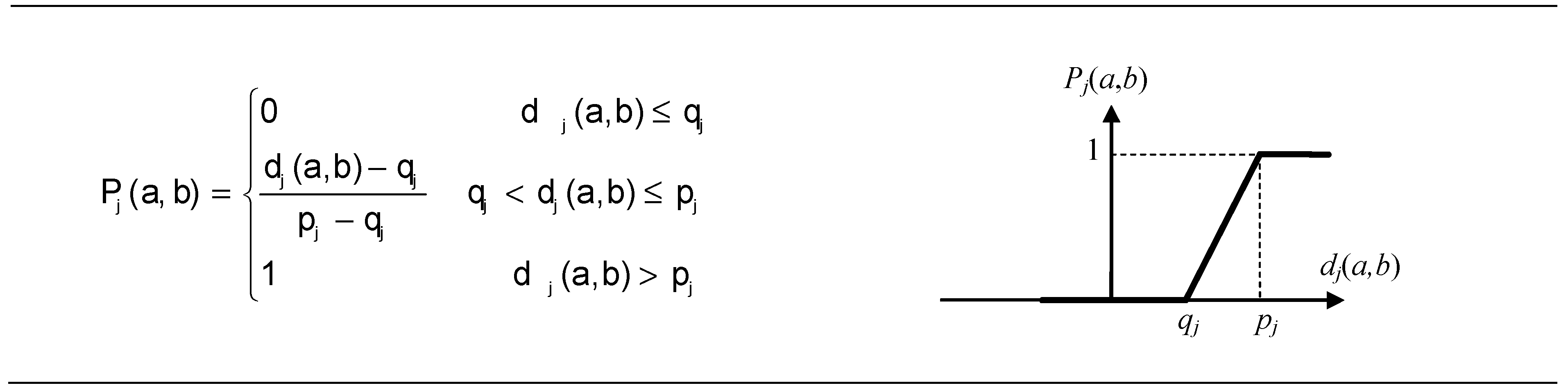
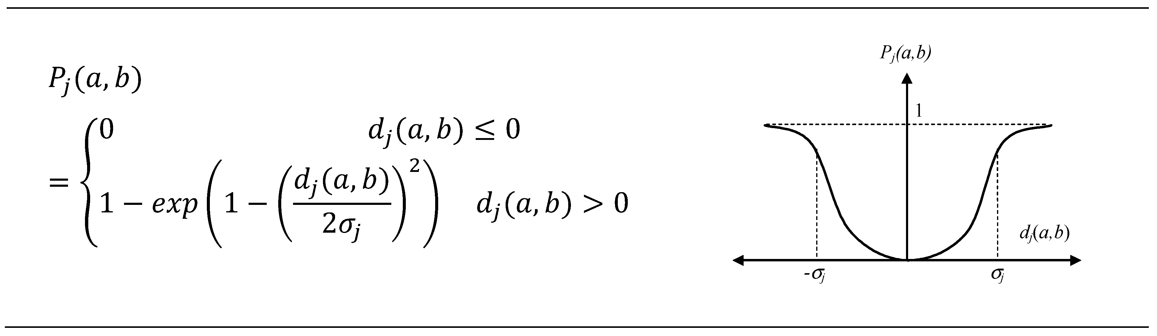
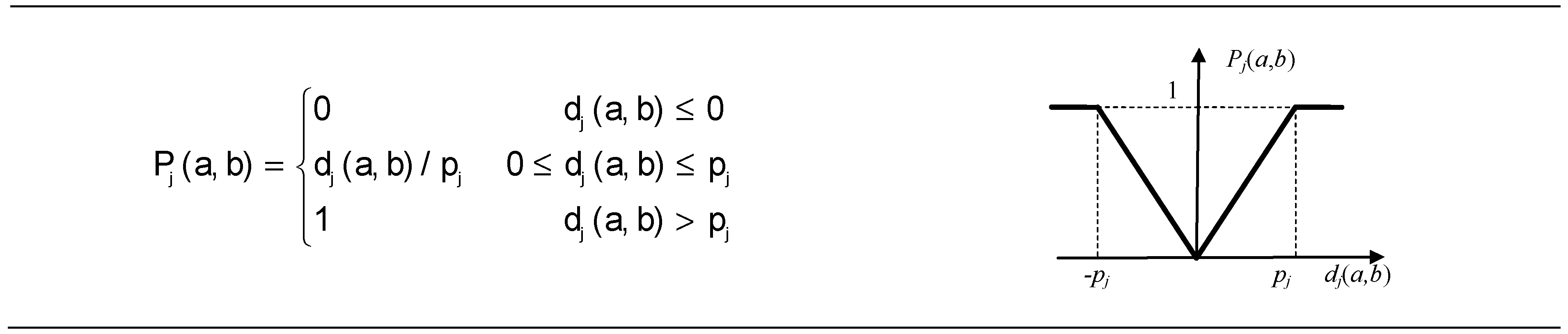
2.6.2. The Preference Function
2.6.3. The Software Packages
3. Results and Discussion
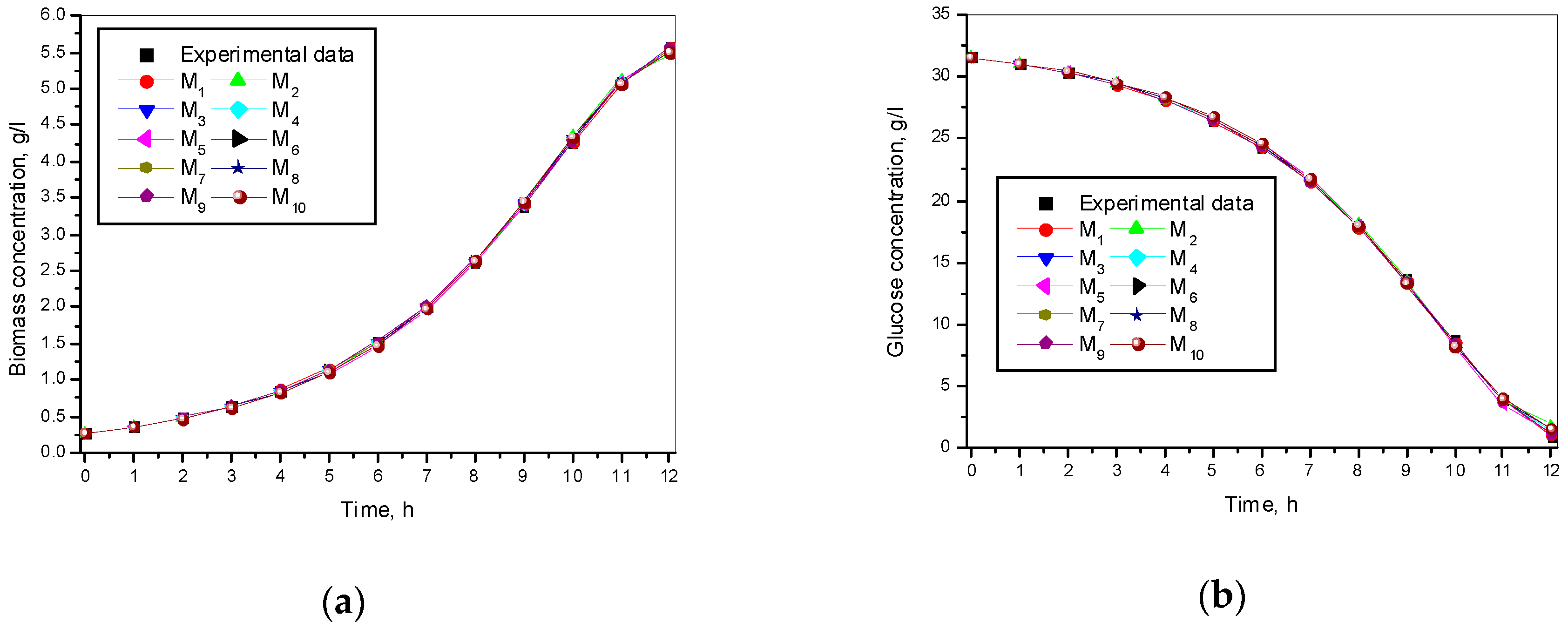
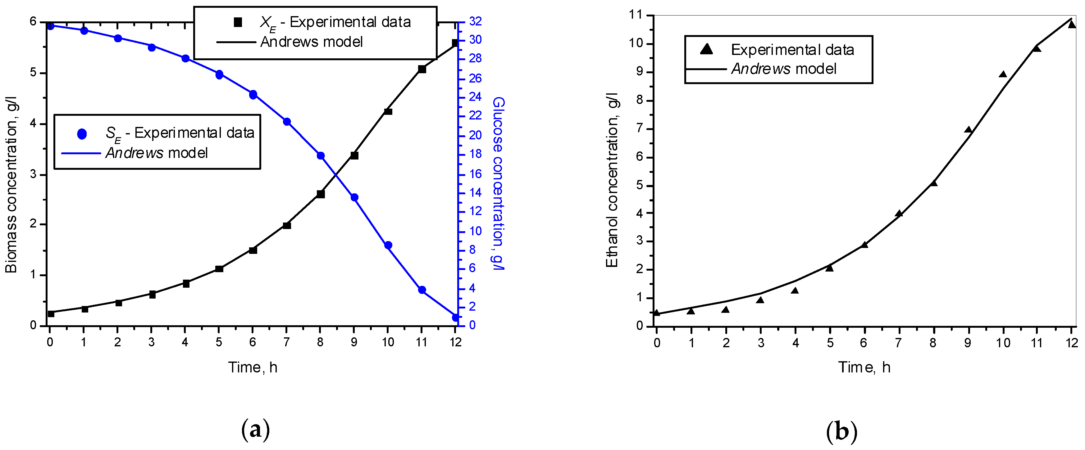
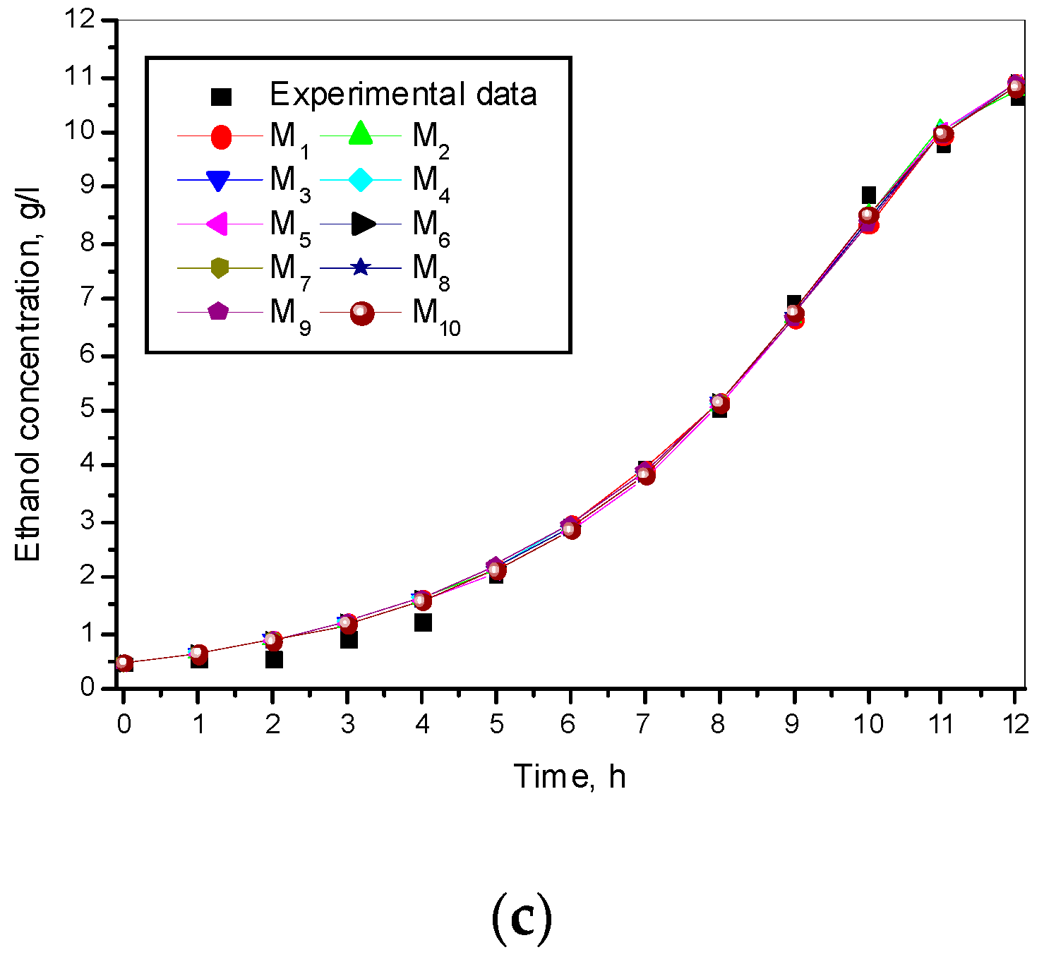
3.1. Results from Modelling
- The criteria C1 changed in the interval C1 ∈ [0.527, 0.646] × 10−3;
- The criteria C2 changed in the interval C2 ∈ [135.863, 186.356]
- The relative errors (criteria C3, C4, C5) for every kinetic variable were changed in the interval C3,4,5 ∈ [0.622, 30.456] × 10−2;
- The Fisher coefficients (criteria C6, C7, C8) were changed in the interval C6, 7, 8 ∈ [1.000, 1.028];
- The correlation coefficient (C9–C11) was changed in the interval C9, 10, 11 ∈ [0.998, 1.000].
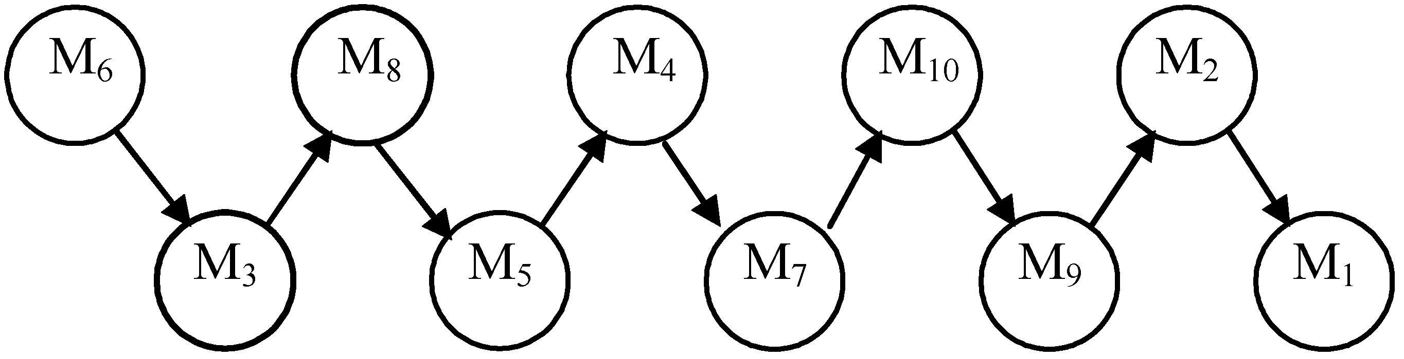
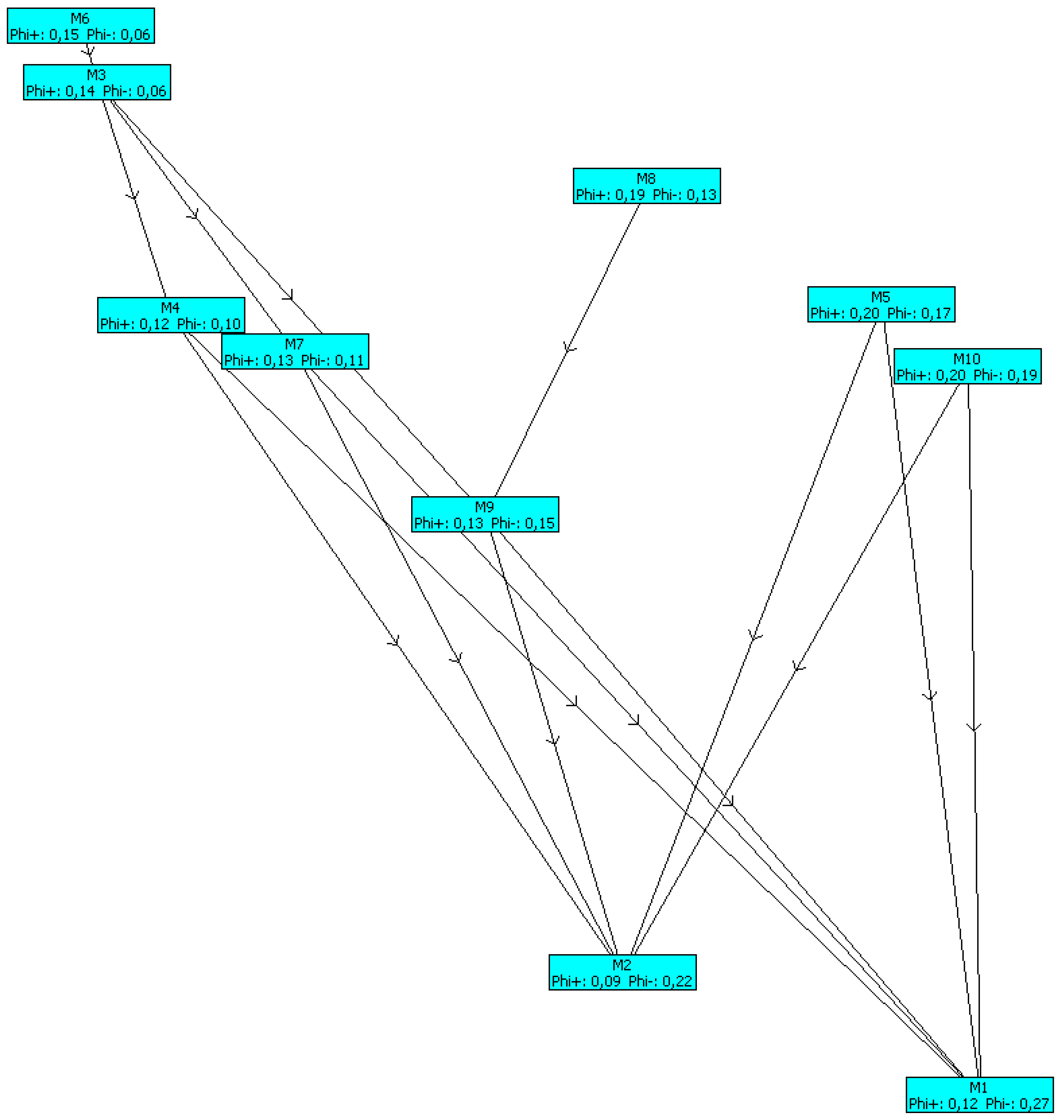
3.2. Application of PROMETHEE II Method
3.2.1. Selection of the Weight
3.2.2. Selection of the Preference Function
3.2.3. The Software Packages
4. Conclusions
Conflicts of Interest
References
- Viesturs, U.; Simeonov, I.; Pencheva, T.; Vanags, J.; Petrov, M.; Pavlov, Y.; Roeva, O.; Ilkova, T.; Vishkins, M.; Hristozov, I. Modelling of yeast fed-batch cultivation using functional state approach. In Contemporary Approaches to Modelling, Optimisation and Control of Biotechnological Processes; Tzonkov, S., Drinov, M., Eds.; Academic Publishing House: Sofia, Bulgaria, 2010; pp. 17–40. [Google Scholar]
- Petrov, M.M.; Ilkova, T.; Roeva, O. Fuzzy-Decision-Making Problems of Fuel Ethanol Production Using a Strain Saccharomyces sereviciae. In The 2010 Research Bulletin of the Australian Institute of High Energetic Materials; Publisher Australian Institute of High Energetic Materials: Queensland, Australia, 2011; pp. 10–28. [Google Scholar]
- Taha, R.A.; Daim, A.T. Multi-Criteria Applications in Renewable Energy Analysis, a Literature Review. In Research and Technology Management in the Electricity Industry. Green Energy and Technology; Daim, T., Oliver, T., Kim, J., Eds.; Springer: London, UK, 2013; pp. 17–30. [Google Scholar] [CrossRef]
- Saaty, R.W. The analytic hierarchy process—What it is and how it is used. Math. Model. 1987, 9, 161–176. [Google Scholar] [CrossRef]
- Figueira, J.; Mousseau, V.; Roy, B. ELECTRE Methods, Multiple Criteria: State of the Art Surveys. In International Series in Operations Research & Management Science; Greco, S., Ed.; Springer: New York, NY, USA, 2005; Volume 78, pp. 133–153. [Google Scholar]
- Dyer, J. MAUT—Multiatribute Utility Theory. In Multiple Criteria: State of the Art Surveys, International Series in Operations Research & Management Science; Greco, S., Ed.; Springer: London, UK, 2005; Volume 78, pp. 265–292. [Google Scholar]
- Brans, J.-P.; Vinke, P. A Preference Ranking Organisation Method (The PROMETHEE method for multiple criteria decision making). Manag. Sci. 1985, 31, 647–656. [Google Scholar] [CrossRef]
- Brans, J.-P.; Mareschal, B. PROMETHEE Methods, Multiple Criteria Decision Analysis: State of the Art Surveys. In International Series in Operations Research & Management Science; Greco, S., Ed.; Springer: London, UK, 2005; Volume 78, pp. 163–195. [Google Scholar]
- Brans, J.-P.; Mareschal, B. The PROMCALC & GAIA decision support system for multicriteria decision aid. Decis. Support Syst. 1994, 12, 297–310. [Google Scholar] [CrossRef]
- Available online: http://www.promethee-gaia.net/assets/bibliopromethee.pdf (accessed on 2 March 2019).
- Viesturs, U.; Berzins, A.; Vanags, J.; Tzonkov, S.; Ilkova, T.; Petrov, M.; Pencheva, T. Application of Different Mixing Systems for the Batch Cultivation of the Saccharomyce cerevisiae. Part I: Experimental Investigations and Modelling. Int. J. Bioautom. 2009, 13, 45–60. [Google Scholar]
- Petrov, M.; Ilkova, T. Modelling of Batch Cultivation of Saccharomyces cerevisiae using Different Mixing Systems. J. Int. Sci. Publ. Mater. Methods Technol. 2014, 8, 3–13. [Google Scholar]
- Viesturs, U.; Berzins, A.; Vanags, J.; Tzonkov, S.; Petrov, M.; Ilkova, T. An Application of Different Mixing Systems for Batch Cultivation of Saccharomyces cerevisiae. Part II: Multiple Objective Optimization and Model Predictive Control. Int. J. Bioautom. 2010, 14, 1–14. [Google Scholar]
- Ilkova, T.; Roeva, O.; Petrov, M. Multiple Objective Optimisation of Batch Cultivation of Saccharomyces cerevisiae in Mixing Systems. Biotechnol. Biotechnol. Equip. 2013, 27, 4162–4166. [Google Scholar] [CrossRef]
- Petrov, M.; Ilkova, T. Modelling and Fuzzy-Decision-Making of Batch Cultivation of Saccharomyces cerevisiae using Different Mixing Systems. Chem. Biochem. Eng. Q. 2014, 28, 531–544. [Google Scholar] [CrossRef]
- Ilkova, T.; Petrov, M. Nonlinear Model Predictive Control of Biotechnological Process for Ethanol Production. J. Int. Sci. Publ. Mater. Methods Technol. 2010, 4 Pt 2, 284–297. [Google Scholar]
- Pencheva, T.; Roeva, O.; Hristozov, I. Description of examined fermentation processes of Saccharomices cerevisiae and Escherichia coli. In Functional State Approach to Fermentation Processes Modelling; Tzonkov, S., Hitzmann, B., Eds.; Academic Publishing House: Sofia, Bulgaria, 2006; pp. 51–56. [Google Scholar]
- Brandt, J.; Hitzmann, B. Knowledge-Based Fault Detection and Diagnosis in Flow-injection Analysis. Anal. Chem. Acta 1994, 291, 29–40. [Google Scholar] [CrossRef]
- Dutta, K.; Venkata, D.V.; Mahanty, B.; Anand Prabhua, A. Substrate inhibition growth kinetics for cutinase producing pseudomonas cepacia using tomato-peel extracted cutin. Biochem. Eng. Q. 2015, 29, 437–445. [Google Scholar] [CrossRef]
- Gera, N.; Uppaluri, R.V.S.; Sen, S.; Venkata Dasuc, V. Growth kinetics and production of glucose oxidase using Aspergillusniger NRRL326. Chem. Biochem. Eng. Q. 2008, 22, 315–320. [Google Scholar]
- Giridhar, R.; Srivastava, A. Model based constant feed fed-batch L-Sorbose production process for improvement in L-Sorbose productivity. Chem. Biochem. Eng. Q. 2000, 14, 133–140. [Google Scholar]
- Kim, D.-J.; Choi, J.-W.; Choi, N.-C.; Mahendran, B.; Lee, C.-E. Modeling of growth kinetics for Pseudomonas spp. during benzene degradation. Appl. Microbiol. Biotechnol. 2005, 69, 456–462. [Google Scholar] [CrossRef] [PubMed]
- Saravanan, P.; Pakshirajan, K.; Saha, P. Kinetics of phenol degradation and growth of predominant Pseudomonas species in a simple batch stirred tank reactor. Bulg. Chem. Commun. 2011, 43, 502–509. [Google Scholar]
- Sudipta, D.; Mukherjee, S. Performance and kinetic evaluation of phenol biodegradation by mixed microbial culture in a batch reactor. Int. J. Water Resour. Environ. Eng. 2010, 2, 40–49. [Google Scholar]
- Chen, Y.; Wang, F.-S. Crisp and Fuzzy Optimization of a Fed-batch Fermentation for Ethanol Production. Ind. Eng. Chem. Res. 2003, 42, 6843–6850. [Google Scholar] [CrossRef]
- Wang, F.-S.; Lin, H.-T. Fuzzy Optimization of Continuous Fermentations with Cell Recycling for Ethanol Production. Ind. Eng. Chem. Res. 2010, 49, 2306–2311. [Google Scholar] [CrossRef]
- Petrov, M.; Ilkova, T. Intercriteria Decision Analysis for Choice of Growth Rate Models of Batch Cultivation by strain Kluyveromyces marxianus var. lactis MC 5. J. Int. Sci. Publ. Mater. Methods Technol. 2016, 10, 468–486. [Google Scholar]
- Macharis, C.; Springael, J.; De Brucker, K.; Verbeke, A. PROMETHEE and AHP: The design of operational synergies in multicriteria analysis. Eur. J. Oper. Res. 2004, 153, 307–317. [Google Scholar] [CrossRef]
- Behzadian, M.; Kazemzadeh, R.B.; Albadvi, A.; Aghdasi, M. PROMETHEE: A comprehensive literature review on methodologies and applications. Eur. J. Oper. Res. 2010, 200, 198–215. [Google Scholar] [CrossRef]
- Available online: http://www.promethee-gaia.net/software.html (accessed on 5 November 2015).
- COMPAQ Visual FORTRAN Programmer’s Guide; v. 6.6; Compaq Computer Corporation: Houston, TX, USA, 2001.
- Vuchkov, I.; Stoyanov, S. Mathematical Modelling and Optimization of Technological Objects; Technique: Sofia, Bulgaria, 1986; pp. 47–50. (In Bulgarian) [Google Scholar]


| Model | Equation | Model | Equation |
|---|---|---|---|
| M1 | M6 | ||
| M2 | M7 | ||
| M3 | M8 | ||
| M4 | M9 | ||
| M5 | M10 |
| Model | µm | KS | KSI | K | Sm | n | m | α | YS/X | YS/E |
|---|---|---|---|---|---|---|---|---|---|---|
| M1 | 0.350 | 6.026 | – | – | – | – | – | – | 0.173 | 0.507 |
| M2 | 0.294 | 25.448 | – | – | – | – | – | – | 0.175 | 0.506 |
| M3 | 0.292 | – | 6.907 | – | – | – | – | – | 0.174 | 0.506 |
| M4 | 0.312 | 10.184 | – | – | – | – | – | 1.422 | 0.174 | 0.507 |
| M5 | 0.852 | 20.000 | 50.000 | – | – | – | – | – | 0.172 | 0.505 |
| M6 | 0.410 | 7.919 | 249.365 | – | – | – | – | – | 0.173 | 0.507 |
| M7 | 0.392 | 7.490 | 287.081 | – | – | – | – | – | 0.173 | 0.507 |
| M8 | 0.771 | 20.000 | – | – | 107.239 | 1.500 | – | – | 0.174 | 0.506 |
| M9 | 0.376 | 6.982 | 671.647 | 81.473 | – | – | – | – | 0.173 | 0.507 |
| M10 | 0.691 | 19.452 | – | – | 69.423 | 1.027 | 0.988 | – | 0.174 | 0.506 |
| Model | C1 × 10−3 | C2 | C3 × 10−2 | C4 × 10−2 | C5 × 10−2 | C6 | C7 | C8 | C9 | C10 | C11 |
|---|---|---|---|---|---|---|---|---|---|---|---|
| M1 | 0.646 | 186.356 | 0.886 | 2.439 | 25.365 | 1.001 | 1.002 | 1.028 | 1.000 | 1.000 | 0.998 |
| M2 | 0.618 | 137.607 | 1.456 | 30.465 | 24.037 | 1.001 | 1.005 | 1.023 | 1.000 | 1.000 | 0.998 |
| M3 | 0.559 | 135.863 | 0.859 | 11.191 | 24.331 | 1.001 | 1.001 | 1.025 | 1.000 | 1.000 | 0.998 |
| M4 | 0.583 | 136.275 | 0.767 | 15.136 | 24.667 | 1.000 | 1.001 | 1.026 | 1.000 | 1.000 | 0.998 |
| M5 | 0.580 | 137.627 | 2.750 | 7.020 | 22.437 | 1.005 | 1.013 | 1.017 | 1.000 | 1.000 | 0.998 |
| M6 | 0.566 | 136.928 | 0.790 | 8.501 | 24.328 | 1.001 | 1.002 | 1.025 | 1.000 | 1.000 | 0.998 |
| M7 | 0.603 | 151.831 | 0.622 | 5.076 | 24.886 | 1.001 | 1.002 | 1.026 | 1.000 | 1.000 | 0.998 |
| M8 | 0.527 | 136.028 | 1.938 | 15.997 | 23.037 | 1.003 | 1.002 | 1.021 | 1.000 | 1.000 | 0.998 |
| M9 | 0.614 | 158.768 | 0.717 | 4.715 | 25.012 | 1.000 | 1.001 | 1.027 | 1.000 | 1.000 | 0.998 |
| M10 | 0.529 | 138.508 | 2.505 | 20.325 | 22.429 | 1.003 | 1.000 | 1.020 | 1.000 | 1.000 | 0.999 |
| Criteria | Min Max | Type of Criteria | Parameters | Criteria | Min Max | Type of Criteria | Parameters |
|---|---|---|---|---|---|---|---|
| C1 | min | VI | σ1 = 0.125 | C6,C7, and C8 | min | III | p6 = 0.003 |
| C2 | σ2 = 16.607 | p7 = 0.008 | |||||
| C3 | σ3 = 0.790 | p8 = 0.007 | |||||
| C4 | σ4 = 8.496 | C9,C10, and C11 | max | V | qj = 5 × 10⁻⁵; pj = 1 × 10⁻³, j = 9, …11 | ||
| C5 | σ5 = 1.044 |
| Rank | Model | φ | φ+ | φ− |
|---|---|---|---|---|
| 1 | M6 | 0.0996 | 0.1622 | 0.0626 |
| 2 | M3 | 0.0821 | 0.1547 | 0.0726 |
| 3 | M8 | 0.0402 | 0.1933 | 0.1531 |
| 4 | M5 | 0.0303 | 0.2237 | 0.1934 |
| 5 | M4 | 0.0284 | 0.1381 | 0.1097 |
| 6 | M7 | 0.0256 | 0.1505 | 0.1249 |
| 7 | M10 | −0.0066 | 0.2087 | 0.2153 |
| 8 | M9 | −0.0135 | 0.1521 | 0.1656 |
| 9 | M2 | −0.1336 | 0.1078 | 0.2414 |
| 10 | M1 | −0.1523 | 0.1346 | 0.2869 |
© 2019 by the author. Licensee MDPI, Basel, Switzerland. This article is an open access article distributed under the terms and conditions of the Creative Commons Attribution (CC BY) license (http://creativecommons.org/licenses/by/4.0/).
Share and Cite
Petrov, M. Modelling and Multi-Criteria Decision Making for Selection of Specific Growth Rate Models of Batch Cultivation by Saccharomyces cerevisiae Yeast for Ethanol Production. Fermentation 2019, 5, 61. https://doi.org/10.3390/fermentation5030061
Petrov M. Modelling and Multi-Criteria Decision Making for Selection of Specific Growth Rate Models of Batch Cultivation by Saccharomyces cerevisiae Yeast for Ethanol Production. Fermentation. 2019; 5(3):61. https://doi.org/10.3390/fermentation5030061
Chicago/Turabian StylePetrov, Mitko. 2019. "Modelling and Multi-Criteria Decision Making for Selection of Specific Growth Rate Models of Batch Cultivation by Saccharomyces cerevisiae Yeast for Ethanol Production" Fermentation 5, no. 3: 61. https://doi.org/10.3390/fermentation5030061
APA StylePetrov, M. (2019). Modelling and Multi-Criteria Decision Making for Selection of Specific Growth Rate Models of Batch Cultivation by Saccharomyces cerevisiae Yeast for Ethanol Production. Fermentation, 5(3), 61. https://doi.org/10.3390/fermentation5030061