Evidence for Glass Behavior in Amorphous Carbon

Abstract

Amorphous carbons are disordered carbons with densities of circa 1.9–3.1 g/cc and a mixture of $s{p}^2$ and $s{p}^3$ hybridization. Using molecular dynamics simulations, we simulate diffusion in amorphous carbons at different densities and temperatures to investigate the transition between amorphous carbon and the liquid state. Arrhenius plots of the self-diffusion coefficient clearly demonstrate that there is a glass transition rather than a melting point. We consider five common carbon potentials (Tersoff, REBO-II, AIREBO, ReaxFF and EDIP) and all exhibit a glass transition. Although the glass-transition temperature ($T_g$) is not significantly affected by density, the choice of potential can vary $T_g$ by up to 40%. Our results suggest that amorphous carbon should be interpreted as a glass rather than a solid.

1. Introduction

Amorphous carbons are often described as one of the allotropes of carbon, along with graphite, diamond and fullerenes. Typically prepared as thin films, amorphous carbons have found numerous technological applications, including wear-resistant coatings on blades and tools, corrosion barriers for hard disks and engine lubrication. For a comprehensive review of the field, summarizing 60 years of research and development, see the review by Vetter [1]. The defining structural characteristics of amorphous carbon are lack of medium- and long-range order, a homogeneous spatial distribution, and a mixture of $s{p}^2$ and $s{p}^3$ hybridization which varies linearly with density. At the highest density of 3.0–3.1 g/cc the $s{p}^3$ fraction is ∼85%, falling to around 10–15% at 1.9 g/cc [2]. Below this density the carbon network develops pores via inhomogeneity and extended order via graphenization. Materials in this category include glassy carbon, nanoporous carbons and foams; none of these materials are considered “amorphous carbons”.

Amorphous carbons can be synthesized using a variety of physical vapor techniques, such as sputtering [3], electron beam evaporation [4], filtered cathodic arc [5,6,7] and mass-selected ion beam [8,9]. The common element in all amorphous carbon synthesis is atom-by-atom impact, whereby a temperature spike generates non-equilibrium deposition conditions that promote the amorphous state. The energy of the depositing atoms (or ions) creates a liquid-like region which persists for a fraction of a picosecond. Even though they form under non-equilibrium conditions, amorphous carbons are typically described as solids as their temperature stability is very high; for example, thin films of tetrahedral amorphous carbon (ta-C) can be heated in vacuum to around 700 ${}^{\circ }$C before structural changes are observed [10,11,12].

The temperatures at which amorphous carbons convert to a liquid are extraordinarily high and have not been accurately determined experimentally. Even basic experimental quantities such as the triple point of carbon are extremely complicated to measure, and the uncertainty in the melting line spans many hundreds of degrees. For a lengthy discussion of the challenges of carbon at high temperature, see the 2015 book by Savvatimskiy [13]. Despite its experimental ambiguity, the liquid state is a convenient starting point to create amorphous carbon in computer simulations. The liquid-quench method is commonly employed in Molecular Dynamics (MD) simulations whereby a carbon liquid is equilibrated at high temperature before being rapidly cooled to create an amorphous solid [14]. The rapid timescale means the liquid-quench scheme is accessible to all forms of MD, from ab initio methods through to empirical potentials.

In this paper, we use MD to study the boundary between amorphous carbon and the liquid state. Using self-diffusion data and an Arrhenius approach, we determine the point at which the low-temperature ”glassy” state (i.e., amorphous carbon) transforms into a high-temperature ”rubbery” state (i.e., liquid carbon). This temperature, which is formally known as the glass-transition temperature ($T_g$), has not previously been computed for carbon. We calculate $T_g$ for five common carbon potentials and consider a range of densities typical for amorphous carbons. We show that $T_g$ values can be easily determined and that they provide a robust alternative to the uncertainty associated with melting behavior in the phase diagram of carbon.

2. Methodology

The simulations are performed using the LAMMPS package [15,16] and complement our recent benchmarking studies of graphitization of amorphous carbons [17,18]. The starting point of the present calculations is a simple cubic lattice containing 4096 atoms. Atoms are randomly displaced by up 0.2 Å in all three Cartesian directions to create a disordered state. It is important that the initial state is high in energy and far from equilibrium. As in our previous works, four densities are considered: 1.5, 2.0, 2.5 and 3.0 g/cc. Periodic boundary conditions are employed and the integration timestep is 0.2 fs. Temperature control is achieved using the Bussi thermostat [19] with a relaxation time of 0.1 ps. Five different interatomic potentials are employed: Tersoff [20], REBO-II [21], AIREBO [22], ReaxFF [23] and EDIP [24]. For a discussion of the merits and history of each potential, see Ref. [17].

All simulations are 80 ps in length and consist of three phases. In the first phase, the NVE ensemble (constant number of particles, volume, energy) is employed and motion is followed for 0.25 ps. During this phase, the lattice spontaneously collapses due to imaginary phonon modes [25] and any correlation with the initial conditions is quickly lost. In the second phase, the NVT ensemble (constant number of particles, volume, temperature) is employed for 4.75 ps to equilibrate the system at the desired temperature. A range of temperatures between 1000 and 9000 K are considered: 20 for the Tersoff potential and 18 for the other potentials. In the third phase, the NVT ensemble is employed for 75 ps to collect data.

3. Results and Discussion

A total of 368 simulations are performed, spanning all combinations of potentials, temperatures and densities. For each simulation the mean-squared-displacement (MSD) is computed every 0.025 ps to extract the self-diffusion coefficient, D. The MSD is defined in the standard way:

$$\mathrm{MSD}\left(t\right)=\frac{1}{N}\sum _{i=1}^N{|{\mathbf{r}}_i\left(t\right)-{\mathbf{r}}_i\left(t_0\right)|}^2$$

(1)

where N is the number of atoms, ${\mathbf{r}}_i$ is the position of atom i, and $t_0$ = 5 ps. In a three-dimensional system D is related to the MSD by the expression $\mathrm{MSD}\left(t\right)=6Dt$, and hence can be extracted via linear regression. To avoid problems with low diffusivity at low temperatures, the fitting procedure only uses data from t = 30 ps onwards.

The results section is divided into two parts. First, we examine in detail a single combination of potential and density, for which we choose the Tersoff potential at 1.5 g/cc. Using this data as an example, we explain the methodology to extract $T_g$. In the second half, we present data using the same analysis for all other potentials and densities.

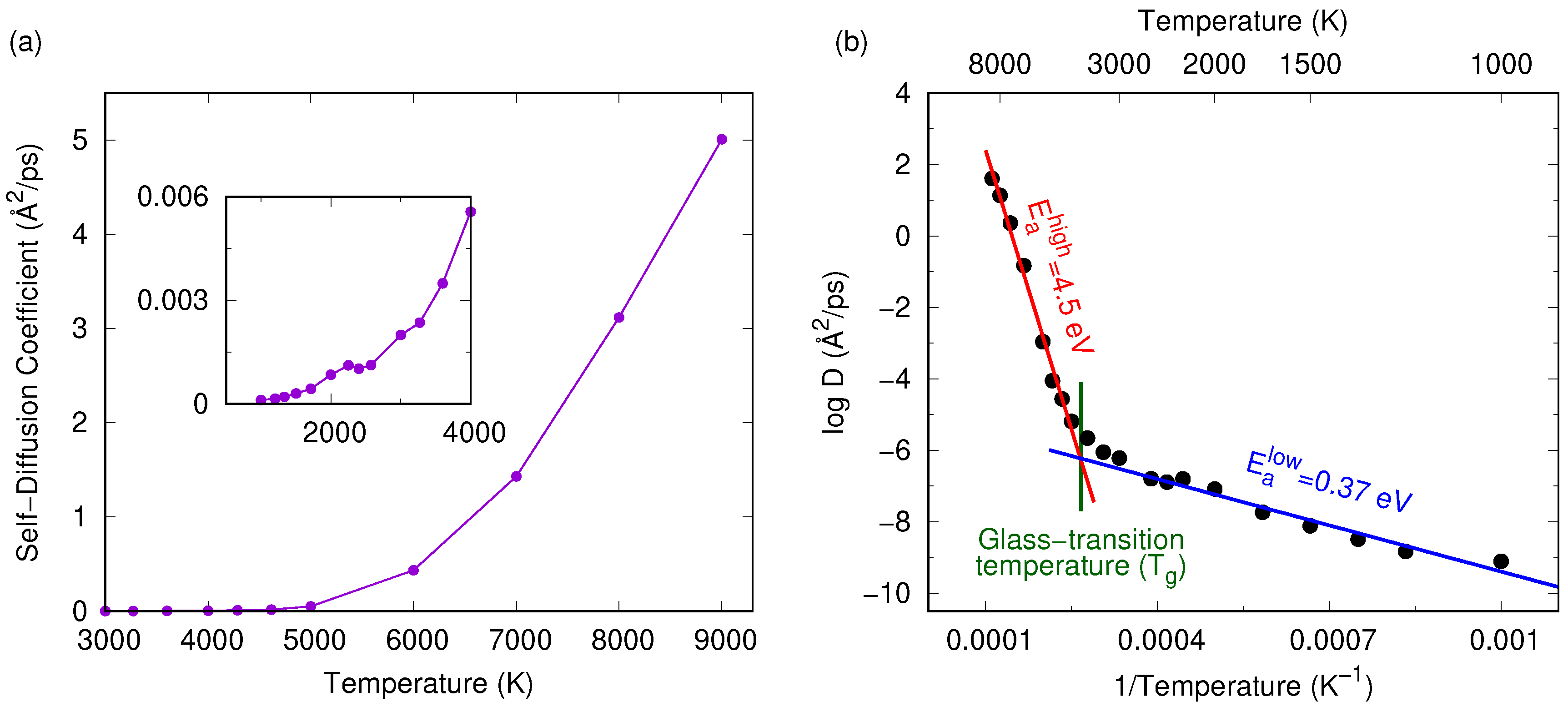
3.1. Tersoff Potential at 1.5 g/cc

The radial distribution function, $g\left(r\right)$, is shown for nine temperatures in Figure 1. The data is an average of 5 snapshots from t = 60 ps to 80 ps, in steps of 5 ps. Panel (a) shows the behavior expected for carbon, with a first-neighbor peak around 1.5 Å, a second-neighbor peak slightly above 2.5 Å and a minimum around 2 Å. At low temperatures there is a clear boundary between the two peaks, and $g\left(r\right)$ goes to zero at the minimum, typical of amorphous carbon. With increasing temperature, both peaks broaden, and eventually the minimum differs significantly from zero, as shown in the inset. These non-zero minima indicate that atoms are moving back-and-forth between the first and second coordination shells, consistent with a liquid phase.

Figure 1b plots the value of $g\left(r\right)$ at the minimum for all temperatures. The main panel uses a linear scale, while the inset is plotted logarithmically. The data in the main panel suggests that liquid behavior commences around 4000 K, while the inset shows that at 3000 K the minima is already non-zero. These values are both significantly lower than the rough estimate of 6000 K for the melting point suggested by Tersoff himself [20]. Due to the lack of a sharp boundary between the liquid and amorphous states, a melting point temperature cannot be defined.

Data for the MSD shown in Figure 2 provides an insightful explanation of the non-zero minimum in $g\left(r\right)$. At the highest temperature of 9000 K (panel (a), grey line) the liquid is highly diffusive as shown by the large positive slope. Under these conditions, atoms easily exchange between the first two coordination shells, as expected in a liquid. As temperature decreases, the slope of the MSD gradually decreases, indicative of less diffusion, but the system remains a liquid. Panel (b) plots the same data as panel (a) but with a greatly reduced range on the vertical scale. At 5000 K (yellow line) the system is clearly still a liquid, while at lower temperatures the slope of the MSD becomes progressively less. Importantly, the MSD never plateaus, indicating that some degree of diffusion is always present.

The self-diffusion coefficient, D, is extracted from the MSD data and is plotted as function of temperature in Figure 3a. The main panel shows behavior consistent with Tersoff’s original estimate of ≈6000 K as the melting point. However, the inset shows that diffusion still occurs at much lower temperatures, and even at 2000 K the value of D is unambiguously non-zero. To explore the dependence of D on temperature, the data is plotted in panel (b) in an Arrhenius manner. This form reveals that the data divides into two linear regimes: a high-temperature region with high diffusivity and a low-temperature region with low diffusivity. In each regime, the activation energy $E_a$ can be determined via an Arrhenius relationship

$$D\left(T\right)=D_{0}exp\left[-\frac{E_a}{k_{B}T}\right]$$

(2)

where $D_0$ corresponds to $D(\infty )$, $k_B$ is Boltzmann’s constant, and T is temperature. The intersection of the two fitted lines defines the glass-transition temperature, $T_g$, and yields a value of 3770 K; this is much higher than commonly accessible temperatures and is consistent with the conventional description of amorphous carbon as a solid. In the high-temperature (“rubbery”) region the activation energy is 4.5 eV, while in the low-temperature (“glassy”) state, the activation energy is more than an order of magnitude smaller, producing a sharp change in slope at $T_g$. This type of behavior is indicative of a second order phase transition, and is observed in materials as diverse as amorphous ice [26], sugar solutions [27] and bulk metallic glasses [28].

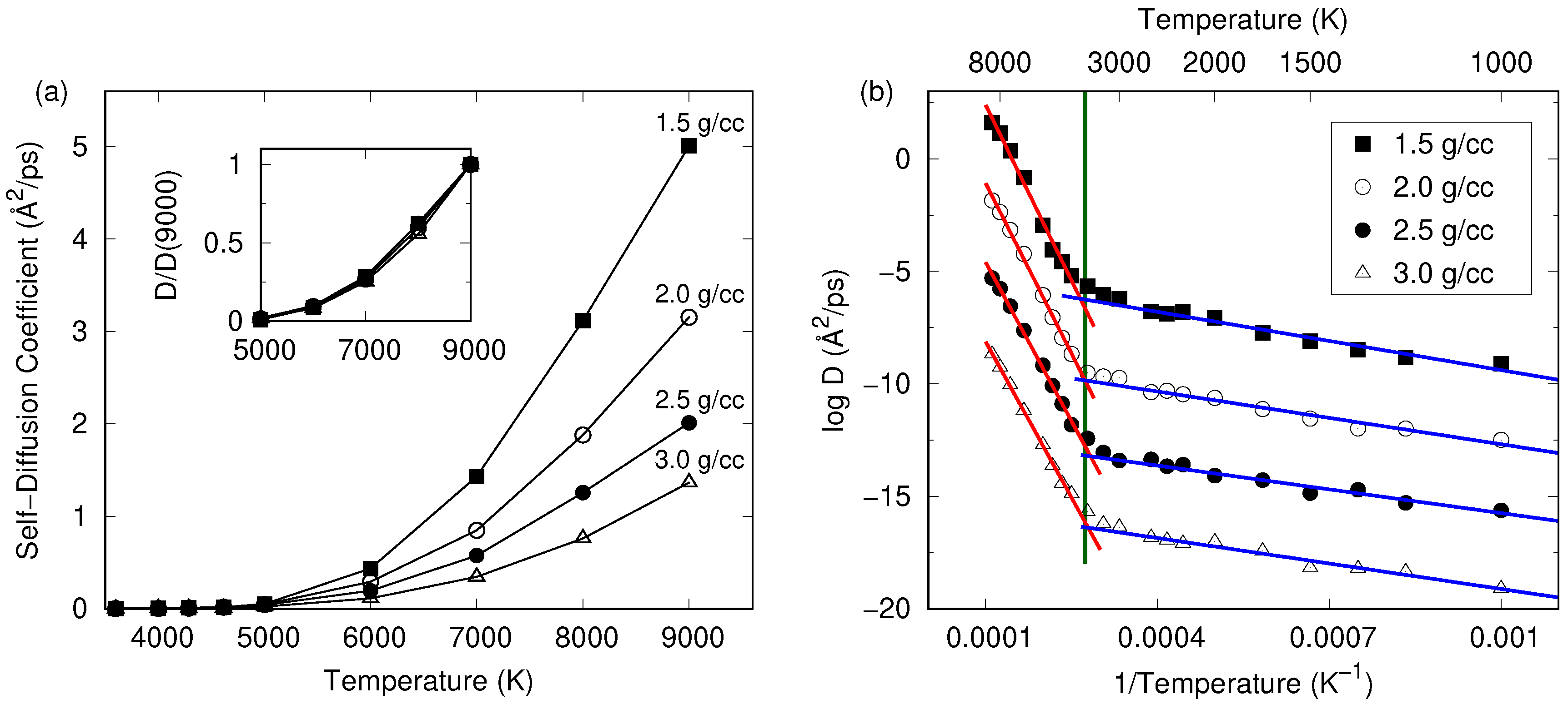
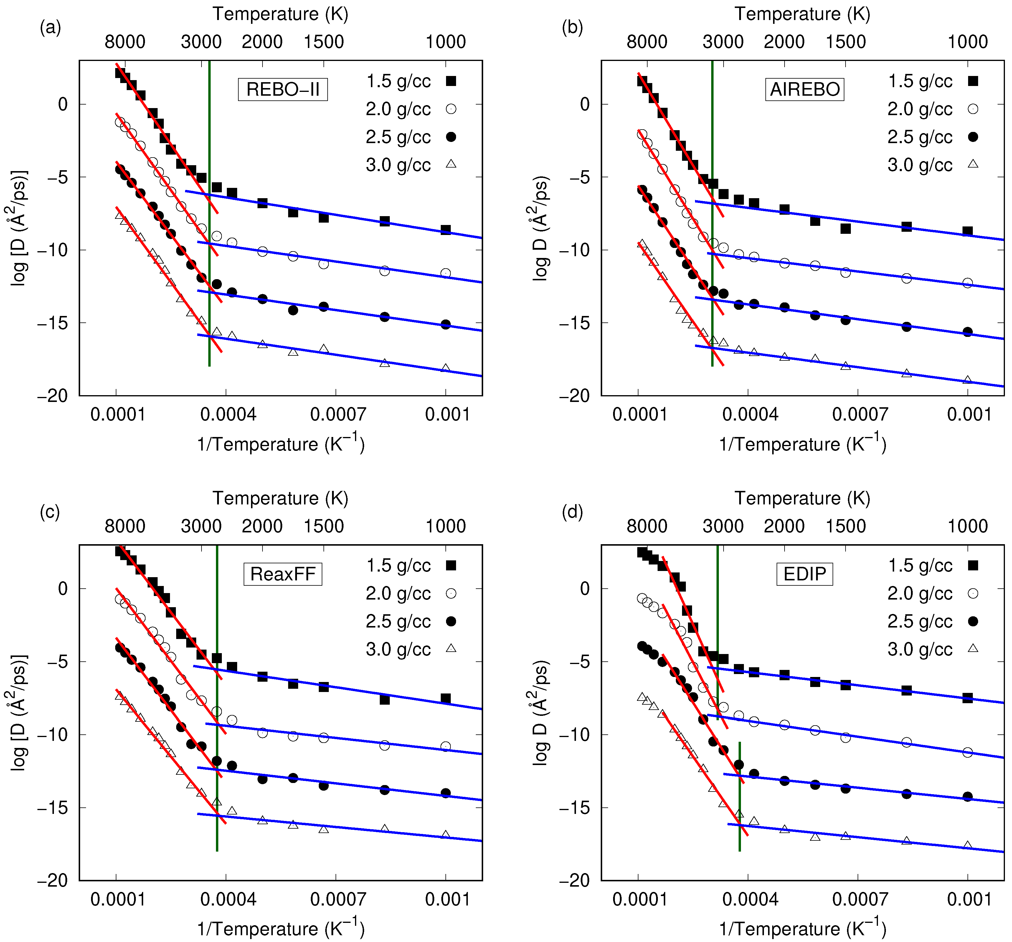
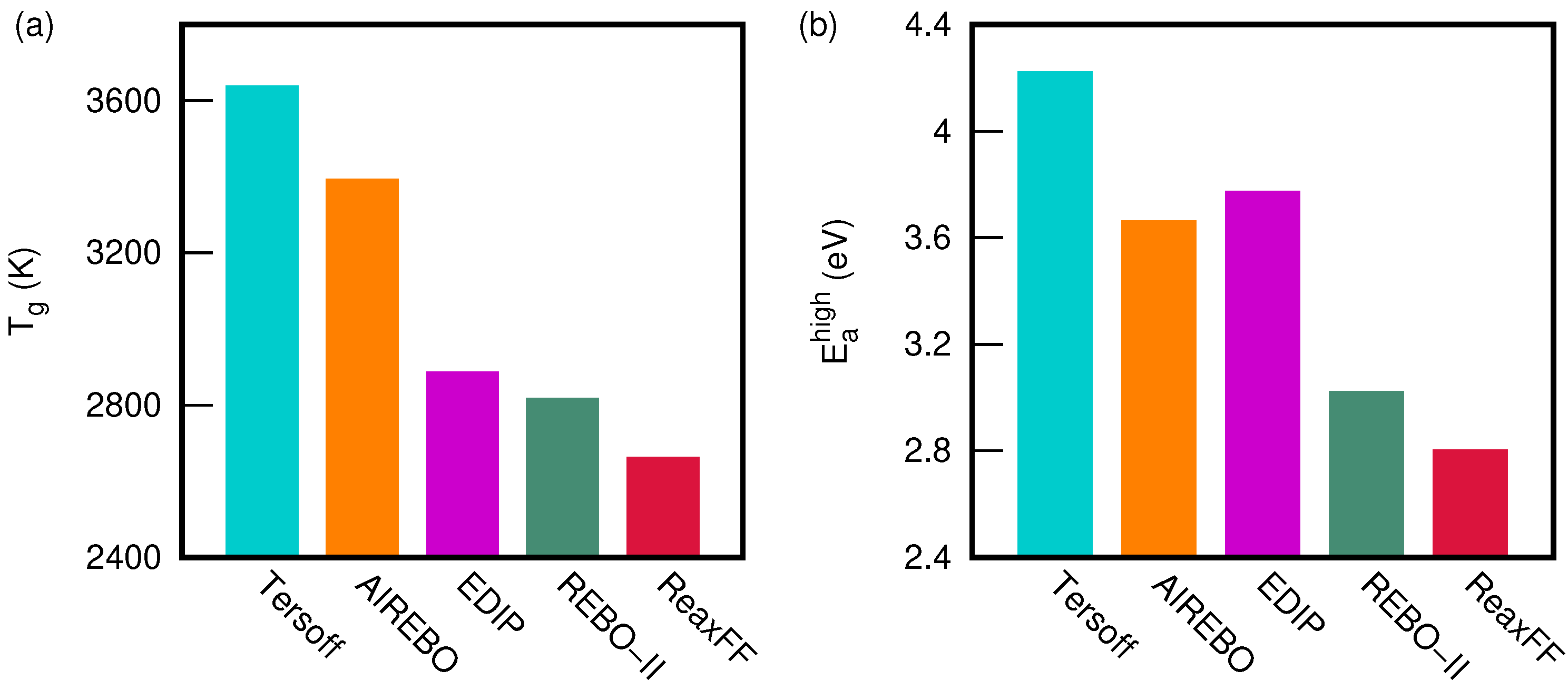
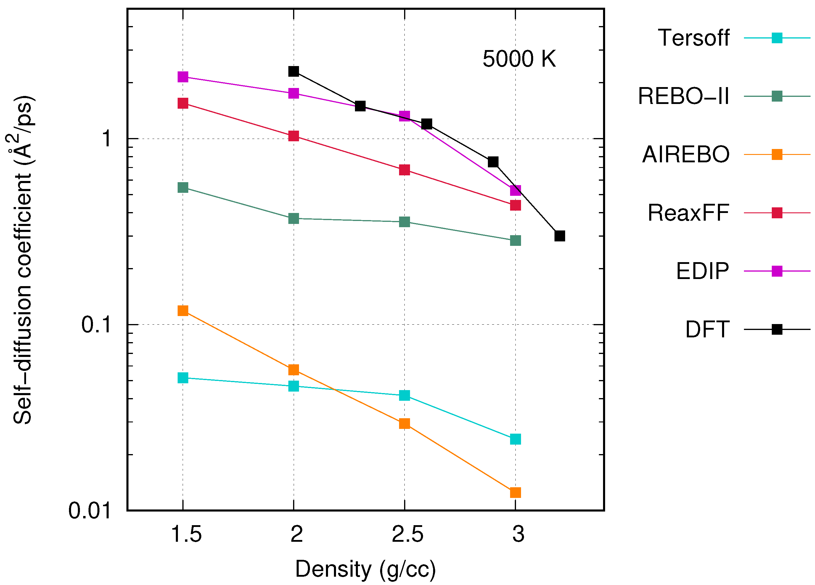
3.2. Comparison between Potentials and Densities

Using the Tersoff potential, the self-diffusion coefficient is computed for three more densities (2.0, 2.5 and 3.0 g/cc) and Figure 4 shows the results. The main plot in panel (a) shows that the self-diffusion constant at a given temperature decreases with density. For example, at 9000 K the value of D reduces by nearly a factor of four between 1.5 and 3.0 g/cc. Across the four densities, the temperature-dependence exhibits a common shape, as shown by the inset which scales the data using the value of D at 9000 K. All the data collapses onto a single line, indicating that the activation energy is not density-dependent.

Figure 4b shows the data in panel (a) in an Arrhenius manner, with the 2.0, 2.5 and 3.0 g/cc data-sets offset by −3, −6 and −9 units in the vertical axis for clarity. Without this offset, the four density data-sets are virtually indistinguishable on a logarithmic scale. The three higher densities exhibit the same behavior seen in Figure 3b, namely two linear regions separated by an abrupt change in slope. The green vertical line indicates that the glass-transition temperature is similar for all four densities and the slopes of the high-temperature region (red line) and low-temperature region (blue line) do not change with density, consistent with the inset in panel (a) where the value of D differs only by a multiplicative factor.

The same analysis is repeated for the other four potentials (REBO-II, AIREBO, ReaxFF and EDIP), and Arrhenius plots for all four densities are shown in Figure 5. Once again, a glass-transition temperature is readily apparent in all data sets. For REBO-II, AIREBO and ReaxFF the value of $T_g$ is roughly the same for all densities, while EDIP shows different behavior, with two distinct $T_g$ values; ∼2600 K at high density and ∼3100 K at low density. Another difference with EDIP is that a second change in slope appears at the very highest temperatures, indicating that the self-diffusion coefficient of the liquid is not characterized by a single activation energy. Close inspection of the 1.5 g/cc data for REBO-II and ReaxFF reveals a hint of a similar change in slope at high temperatures. The origin of this behavior is unclear.

The full data-set of $T_g$ values and activation energies for all potentials and densities are listed in

Table 1. Glass-transition temperature ($T_g$), and activation energies of disordered carbons for the five potentials and four densities. Uncertainties are 95% confidence limits determined from the regression analysis.

Potential	Density (g/cc)	${\mathit{T}}_{\mathit{g}}$ (K)	${\mathit{E}}_{\mathit{a}}^{\mathit{high}}$ (eV)	${\mathit{E}}_{\mathit{a}}^{\mathit{low}}$ (eV)
Tersoff	1.5	3770 ± 370	4.49 ± 0.30	0.37 ± 0.06
	2.0	3660 ± 230	4.35 ± 0.18	0.34 ± 0.05
	2.5	3530 ± 220	4.06 ± 0.15	0.30 ± 0.06
	3.0	3580 ± 210	3.98 ± 0.13	0.33 ± 0.05
REBO-II	1.5	2930 ± 370	3.20 ± 0.24	0.34 ± 0.10
	2.0	2830 ± 240	3.03 ± 0.11	0.31 ± 0.09
	2.5	2710 ± 260	2.89 ± 0.14	0.31 ± 0.09
	3.0	2800 ± 310	2.97 ± 0.20	0.32 ± 0.08
AIREBO	1.5	3210 ± 350	3.66 ± 0.09	0.27 ± 0.14
	2.0	3360 ± 130	3.80 ± 0.06	0.26 ± 0.05
	2.5	3420 ± 160	3.59 ± 0.06	0.29 ± 0.05
	3.0	3570 ± 220	3.59 ± 0.15	0.29 ± 0.03
ReaxFF	1.5	2720 ± 470	2.86 ± 0.32	0.32 ± 0.11
	2.0	2620 ± 400	2.87 ± 0.30	0.24 ± 0.10
	2.5	2680 ± 380	2.85 ± 0.26	0.25 ± 0.10
	3.0	2620 ± 300	2.64 ± 0.17	0.21 ± 0.10
EDIP	1.5	3190 ± 840	4.39 ± 0.86	0.26 ± 0.03
	2.0	3050 ± 740	4.13 ± 0.75	0.31 ± 0.04
	2.5	2660 ± 570	3.43 ± 0.57	0.22 ± 0.06
	3.0	2630 ± 290	3.12 ± 0.22	0.22 ± 0.09

. The uncertainties are obtained from the regression fitting and indicate 95% confidence limits (i.e., 1.96 × the standard error in the mean). Despite these uncertainties, clear trends are evident across the densities and between the potentials. The quantity showing the least variability in Table 1 is the low-temperature activation energy ($E_a^{low}$) which is roughly constant for all potentials and densities. This can be seen visually in Figure 4 and Figure 5 where the blue lines have similar slopes for all potentials. The activation energy at high temperature ($E_a^{high}$) shows a larger spread of values, from as little as 2.6 eV for ReaxFF at 3.0 g/cc to as high as 4.5 eV for Tersoff at 1.5 g/cc. However, for an individual potential the value is fairly constant across the four densities. The largest variation occurs for EDIP, while for the other potentials the variation is only a few tenths of an eV. Regarding $T_g$, the somewhat large confidence intervals provided in Table 1 reflect the propagation of uncertainties from the two linear fitting regions in the Arrhenius plot. As can be seen graphically in Figure 4 and Figure 5, the $T_g$ values for the Tersoff, REBO-II and ReaxFF potentials are nearly constant for the four densities. For AIREBO, Table 1 shows that $T_g$ exhibits slightly more variation, increasing monotonically with density. For EDIP, the $T_g$ values may be separated into two groups, albeit with rather large uncertainties (≈800 K) for the two lower densities due to the small number of points contributing to the linear fit.

To assess the broad trends in the data of Table 1 it is helpful to average across the four densities and condense the $T_g$ and activation energies to a single value for each potential. In the case of $E_a^{low}$, a value of ∼0.3 eV represents well all five potentials. Although this activation energy is small, indicating only a small temperature-dependence, it is unambiguously non-zero and therefore not a solid. On the other hand, $T_g$ and $E_a^{high}$ vary significantly across the five potentials, as seen in Figure 6. The average $T_g$ value of 3640 K for the Tersoff potential is nearly 40% larger than the corresponding value of 2660 K for ReaxFF, while the difference for $E_a^{high}$ is 50% (4.22 eV for Tersoff versus 2.80 eV for ReaxFF). In panel (a) the potentials are arranged in decreasing value of $T_g$, and employing the same order in panel (b) shows that $T_g$ and $E_a^{high}$ are correlated. These variations demonstrate that the energy barriers for bond-making and bond-breaking in liquid carbon differ substantially between potentials, and reflect the differing types of functional forms and parametrization. It is particularly interesting that the REBO-II and AIREBO potentials differ so substantially in their $T_g$ and $E_a^{high}$ values, given that AIREBO is closely related to REBO, differing only in the addition of a $1/r^6$ term to describe van der Waals attraction between $s{p}^2$-bonded layers. A plausible explanation for this AIREBO/REBO-II difference is that the switching function used in AIREBO to disable the $1/r^6$ term at short distances introduces additional energy barriers not present in REBO-II, thereby increasing both $E_a^{high}$ and $T_g$.

Aside from noting the obvious differences between potentials, it is instructive to numerically interpret the data in Figure 6. In the case of the activation energy, the $E_a^{high}$ values are close to the bond dissociation energy of a carbon $\sigma$-bond, which is 3.9 eV in n-alkanes [29] and 3.7 eV in diamond [30]. This resemblance is not unreasonable given that liquid carbon fundamentally involves breaking of bonds. This correspondence between activation energy and bond strength is also found in amorphous silicon where experiments [31] show that the self-diffusion constant also follows an Arrhenius relation. The measured value of $E_a$ is 2.7 eV, of similar order to the dissociation energy of a silicon $\sigma$-bond (2.3 eV [30]).

It is initially puzzling to compare the $T_g$ values in Figure 6a to empirical observations of melting in MD simulations. For example, Tersoff estimated ≈6000 K as the melting point with his potential, while in our EDIP simulations we have observed that 4300–4500 K is a typical temperature at which melting occurs. Both estimates are much larger than the respective $T_g$ values. Insight into this large difference comes from the field of polymers, where there is an empirical relation that $T_g/T_m\sim 2/3$ [32], where $T_m$ is the melting point. Although we cannot properly define $T_m$ for amorphous carbon thermodynamically, this relationship implies a melting temperature around 1.5 times the $T_g$ value. Using $T_g$ of 3640 K for Tersoff and 2880 K for EDIP we can estimate $T_m$ values of 5500 K and 4300 K, respectively, both of which match with empirical observations. Applying the same procedure for the other three potentials yields $T_m$ estimates of 4200, 5100 and 4000 K for REBO-II, AIREBO and ReaxFF, respectively. This approach provides a convenient and robust way to estimate melting temperatures.

The large differences in melting temperatures raises the question as to which (if any) of the potentials is correct. In the absence of experimental results, Density-Functional-Theory (DFT) is the best source of data for validation. Zhao et al. [33] used the VASP package to perform DFT calculations of liquid carbon at a range of densities, and reported a self-diffusion coefficient of 3.42 Å${}^2$/ps at 7500 K for a 2.96 g/cc system. Averaging the 7000 and 8000 K self-diffusion coefficients for our 3.0 g/cc system yields values of 0.22, 0.55, 2.04, 2.71 and 2.91 Å${}^2$/ps for AIREBO, Tersoff, REBO-II, ReaxFF and EDIP, respectively. AIREBO and Tersoff are around an order of magnitude too small, while of the other potentials, EDIP is the closest. We have previously computed DFT data for liquid carbon at a range of densities at 5000 K. The calculations were performed using the CPMD code and contained 125 atoms; the methodology is described in Ref. [34]. Figure 7 compares this DFT data with all five potentials at 5000 K. Once again, the largest discrepancy is seen for Tersoff and AIREBO, where the diffusion is nearly two orders of magnitude too small. This low diffusivity correlates with the data in Figure 6a, where Tersoff and AIREBO have by far the highest $T_g$ values. The best agreement with DFT is found for ReaxFF and EDIP. These two potentials were developed with energy barriers in mind, which helps to explain the better description of the liquid phase. It is worth noting that these two potentials performed the best in our benchmarking studies of graphitization [17,18].

4. Conclusions

This work relates to one of the important objectives for carbon science as pointed out by Prof. Rodney Ruoff in 2018 [35]. He encouraged experimental and theoretical study of the carbon phase diagram to achieve a complete understanding. Our contribution is to show that amorphous carbon has a well-defined glass-transition temperature ($T_g$). Even though amorphous carbon is often described as a solid, it clearly displays glass behavior, as demonstrated by a sharp change in slope in Arrhenius plots of the self-diffusion coefficient. Unfortunately, renaming amorphous carbon as carbon glass is not an option, as the term “glassy carbon” is already in use, describing high-temperature vitreous carbons that have a shiny, or “glassy” appearance.

A practical output from this work is a simple methodology to calculate $T_g$ from molecular dynamics. This approach provides a useful piece of information to benchmark carbon potentials, where the melting temperature varies substantially between potentials. Comparison with DFT data shows that EDIP and ReaxFF provide the best description of the liquid state. Using the empirical relationship $T_m\approx 1.5\times T_g$, we can estimate a melting temperature of carbon of ≈4300 K, as predicted by EDIP. Although this melting temperature is not thermodynamically well defined, it has practical value in high-temperature simulations. For example, in liquid-quench simulations used to prepare amorphous carbon structures, the liquid needs to be equilibrated well above the melting temperature. In other cases, such as studying graphitization associated with Joule heating, the chosen temperature needs to be sufficiently high to enable rearrangement, but below the melting temperature.