Deep Reinforcement Learning for Fluid Mechanics: Control, Optimization, and Automation

Abstract

A comprehensive review of recent advancements in applying deep reinforcement learning (DRL) to fluid dynamics problems is presented. Applications in flow control and shape optimization, the primary fields where DRL is currently utilized, are thoroughly examined. Moreover, the review introduces emerging research trends in automation within computational fluid dynamics, a promising field for enhancing the efficiency and reliability of numerical analysis. Emphasis is placed on strategies developed to overcome challenges in applying DRL to complex, real-world engineering problems, such as data efficiency, turbulence, and partial observability. Specifically, the implementations of transfer learning, multi-agent reinforcement learning, and the partially observable Markov decision process are discussed, illustrating how these techniques can provide solutions to such issues. Finally, future research directions that could further advance the integration of DRL in fluid dynamics research are highlighted.

1. Introduction

The mechanisms through which the human brain acquires and incorporates knowledge have long been intriguing research topics. Emulating such abilities through self-developing algorithms has become a primary goal in machine learning. Reinforcement learning (RL) is a framework in which an agent learns to make decisions by interacting with the environment, aiming to maximize cumulative reward through trial and error, akin to human learning [1]. Since its inception, RL has shown considerable potential [2], although its applications have traditionally been confined to low-dimensional problems. However, the advent of deep reinforcement learning (DRL) represents a significant advancement, integrating deep neural networks (DNNs) with RL algorithms. DRL leverages the capacity of DNNs to approximate nonlinear functions in high-dimensional spaces [3], leading to groundbreaking achievements in various fields such as robotics [4], autonomous driving [5,6], natural language processing [7], and gaming [8,9,10].

The field of fluid mechanics also struggles with challenges due to the nonlinear and high-dimensional nature of fluid motions governed by the Navier–Stokes equations. The ability of DRL to address complex decision-making problems offers new possibilities for fluid dynamics research. Common applications of DRL in fluid mechanics include flow control and shape optimization. Flow control aims to appropriately alter system dynamics to achieve desirable performance. An early and widely studied example is drag reduction for a two-dimensional cylinder, which now serves as a benchmark case for validating DRL-based flow control methods [11,12,13,14,15,16,17,18,19,20,21,22,23,24]. In shape optimization, DRL agents modify geometries to optimize specific objective functions. A classical example is the optimization of airfoil shapes to enhance aerodynamic characteristics, such as reducing drag or increasing lift [25,26,27,28,29,30,31]. These foundational applications demonstrate the potential of DRL to resolve fluid dynamics problems that were previously intractable with conventional methods.

However, a variety of challenges have emerged as DRL-based research in fluid dynamics advances to tackle more intricate real-world problems. The most prominent challenge is the computational cost of acquiring data. The computational cost needed to evaluate system dynamics escalates as geometries and flow conditions become more complex. This issue is especially pronounced when dealing with turbulent flow regimes, where the multi-scale nature of turbulent flow requires extensive data to accurately capture down to small-scale motions. Moreover, the inherent stochasticity of turbulence introduces high variance in the training data, negatively impacting both the performance and robustness of DRL algorithms. The partial observability of the state space further complicates the problem, necessitating techniques to effectively utilize incomplete information. Consequently, the recent research trend is to adopt supplementary strategies alongside DRL algorithms to address these challenges effectively.

The aim of the present paper is to provide a comprehensive review of recent literature on the application of DRL to fluid dynamics problems. Earlier reviews of DRL-based research in fluid mechanics were introduced by Rabault et al. [32] and updated by Garnier et al. [33] and Viquerat et al. [34]. Vignon et al. [35] focused on studies utilizing DRL with an emphasis on flow control. Compared to the previous reviews, the present review concentrates on the strategies employed in recent research to address the challenges encountered when applying DRL to more complex fluid dynamics problems. Specifically, transfer learning, multi-agent reinforcement learning (MARL), and the partially observable Markov decision process (POMDP) are discussed, detailing how these techniques can provide solutions to such issues. Additionally, unlike previous reviews that primarily focused on flow control and shape optimization, the current review introduces research trends in the automation of computational fluid dynamics (CFD), a newly emerging field that holds promise for advancing the efficiency and reliability of numerical analysis.

The paper is organized as follows: The theoretical background and the main DRL algorithms applied in fluid dynamics research are described in Section 2. The challenges encountered in DRL-based fluid dynamics research and the strategies used to address these issues are explained in Section 3. Comprehensive reviews of the applications in flow control, shape optimization, and automation of CFD are provided in Section 4, Section 5 and Section 6, respectively, followed by concluding remarks in Section 7.

2. Deep Reinforcement Learning

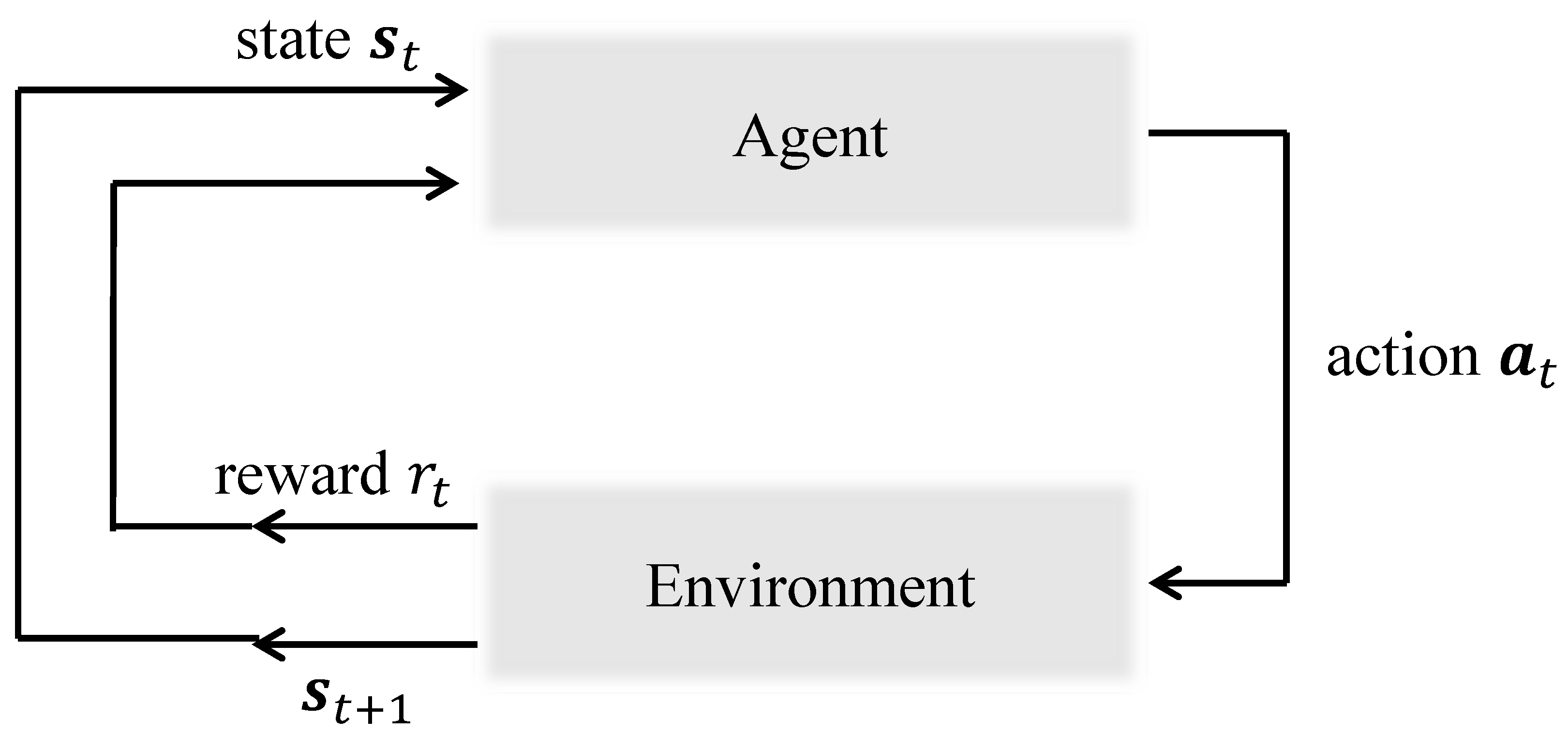
RL is a framework for acquiring an optimal strategy in a sequential decision-making process [1]. In the general RL problem, the process is often modeled as a Markov decision process (MDP), where an agent interacts with the environment, as illustrated in Figure 1. At each step t, a state ${\mathbf{s}}_t\in \mathcal{S}$ is given to the agent by the environment, and the agent executes an action ${\mathbf{a}}_t\in \mathcal{A}$ according to its policy $\mathbf{\pi }$, where $\mathcal{S}$ and $\mathcal{A}$ refer to the state and action spaces, respectively. Subsequently, a reward $r_t({\mathbf{s}}_t,{\mathbf{a}}_t)\in \mathbb{R}$ is obtained, and the state transitions to ${\mathbf{s}}_{t+1}$. The probability of transitioning to the next state ${\mathbf{s}}_{t+1}$ is determined by the state transition function $T({\mathbf{s}}_t,{\mathbf{a}}_t,{\mathbf{s}}_{t+1}):\mathcal{S}\times \mathcal{A}\times \mathcal{S}\to [0,1]$, and the reward is defined by the reward function $R({\mathbf{s}}_t,{\mathbf{a}}_t,{\mathbf{s}}_{t+1}):\mathcal{S}\times \mathcal{A}\times \mathcal{S}\to \mathcal{R}$, where $\mathcal{R}$ denotes a set of possible rewards. The procedure continues to the terminal step T, where one episode ends. The goal of the agent is to discover an optimal policy that maximizes the discounted cumulative reward, denoted as the return $G_t$, which is defined as follows:

$$G_t=\sum _{i=t}^T{\gamma }^{(i-t)}{r}_i({\mathbf{s}}_i,{\mathbf{a}}_i),$$

(1)

where $\gamma \in [0,1)$ is a discount factor that defines the weight between long-term and short-term rewards.

To train the agent, value functions are utilized to evaluate the performance of the policy. The state value function $V^{\mathbf{\pi }}\left(\mathbf{s}\right)$ is defined as the expected return as follows:

$$V^{\mathbf{\pi }}\left(\mathbf{s}\right)={\mathbb{E}}_{\mathbf{\pi }}\left[G_t\right|{\mathbf{s}}_t=\mathbf{s}].$$

(2)

Similarly, the action value function $Q^{\mathbf{\pi }}(\mathbf{s},\mathbf{a})$ is defined as follows:

$$Q^{\mathbf{\pi }}(\mathbf{s},\mathbf{a})={\mathbb{E}}_{\mathbf{\pi }}\left[G_t\right|{\mathbf{s}}_t=\mathbf{s},{\mathbf{a}}_t=\mathbf{a}].$$

(3)

In Equations (2) and (3), the expectation is taken over the policy $\mathbf{\pi }$ with environment transitions. The optimal policy ${\mathbf{\pi }}^{*}$ refers to the policy achieving optimal value functions, as follows:

$$V^{*}\left(\mathbf{s}\right)=\underset{\mathbf{\pi }}{max}{V}^{\mathbf{\pi }}\left(\mathbf{s}\right),$$

(4)

$$Q^{*}(\mathbf{s},\mathbf{a})=\underset{\mathbf{\pi }}{max}{Q}^{\mathbf{\pi }}(\mathbf{s},\mathbf{a}).$$

(5)

In early RL algorithms, tables were utilized to calculate policy measures such as the value functions by storing the values for every state–action pair. However, such an approach can easily become intractable with the increasing dimensions of state and action spaces. DRL incorporates deep learning techniques, leveraging the capacity of artificial neural networks to approximate complex functions and learn from high-dimensional inputs using nonlinear activation functions. This capability is particularly advantageous for fluid mechanics problems, where the dynamics are challenging due to the nonlinear and high-dimensional nature of fluid motions. Based on whether the neural network is used to approximate value functions or directly map policies, DRL algorithms can be categorized as value-based methods and policy-based methods, respectively.

2.1. Value-Based Methods

Value-based methods utilize neural networks to approximate value functions, from which the policy is derived. One of the most popular value-based algorithms is Q-learning [36], which aims to learn the action-value function in Equation (3) to obtain an optimal policy. To achieve the optimal action-value function, the Bellman optimality equation is employed as follows:

$$Q^{*}(\mathbf{s},\mathbf{a})=\sum _{{\mathbf{s}}^{\prime }\in \mathcal{S}}T(\mathbf{s},\mathbf{a},{\mathbf{s}}^{\prime })\left(R(\mathbf{s},\mathbf{a},{\mathbf{s}}^{\prime })+\gamma \underset{{\mathbf{a}}^{\prime }}{max}{Q}^{*}({\mathbf{s}}^{\prime },{\mathbf{a}}^{\prime })\right).$$

(6)

In the early version of Q-learning, a Q-table is used to store the values of the action-value function for every state–action pair, with values gradually updated until Equation (6) is satisfied. The optimal policy is then achieved as follows:

$${\mathbf{\pi }}^{*}\left(\mathbf{s}\right)=\underset{\mathbf{a}}{argmax}{Q}^{*}(\mathbf{s},\mathbf{a}).$$

(7)

Deep Q-networks. The use of a Q-table becomes intractable as the dimensions of the state and action spaces increase in Q-learning. Deep Q-networks (DQN) [8,37] address this challenge by using neural networks to approximate the action-value function as $Q_{\mathit{\theta }}(\mathbf{s},\mathbf{a})$, where $\mathit{\theta }$ denotes the network parameters. The network parameters are updated using a gradient descent algorithm to minimize the loss function derived from Equation (6) as follows:

$$L\left(\mathit{\theta }\right)={\mathbb{E}}_{(\mathbf{s},\mathbf{a},r,{\mathbf{s}}^{\prime })\sim \mathcal{D}}\left[{\left(r+\gamma \underset{{\mathbf{a}}^{\prime }}{max}{Q}_{{\mathit{\theta }}^{-}}({\mathbf{s}}^{\prime },{\mathbf{a}}^{\prime })-Q_{\mathit{\theta }}(\mathbf{s},\mathbf{a})\right)}^2\right].$$

(8)

Two key techniques are employed to improve stability and convergence. Firstly, a target network is used to stabilize the training process by periodically updating its parameters ${\mathit{\theta }}^{-}$ to match the main network $\mathit{\theta }$. Secondly, the experience replay buffer $\mathcal{D}$ stores transition tuples $(\mathbf{s},\mathbf{a},r,{\mathbf{s}}^{\prime })$, which are sampled randomly to break the correlation between successive updates. For action selection, the $ϵ$-greedy strategy is employed to balance exploration and exploitation. The agent chooses a random action with probability $ϵ$ and, otherwise, executes the optimal action of ${argmax}_{\mathbf{a}}{Q}_{\mathit{\theta }}(\mathbf{s},\mathbf{a})$. Various algorithms and techniques continue to improve the performance of DQN, including double DQN [38], dueling DQN [39], prioritized replay DQN [40], and rainbow DQN [41].

2.2. Policy-Based Methods

When dealing with high-dimensional or continuous action spaces, value-based methods become computationally inefficient due to the need for an extensive number of discretizations of the action space. Policy-based methods address this issue by directly mapping the policy using neural networks with parameters $\mathit{\theta }$ as ${\mathbf{\pi }}_{\mathit{\theta }}$. The objective is to maximize the expected return, defined as $J\left(\mathit{\theta }\right)={\mathbb{E}}_{\mathbf{\pi }}\left[G_t\right]$, by adjusting the parameters using a gradient ascent algorithm as follows:

$$\mathit{\theta }\leftarrow \mathit{\theta }+\alpha {\nabla }_{\mathit{\theta }}J\left(\mathit{\theta }\right),$$

(9)

where $\alpha$ represents a learning rate. Policy-based methods can be categorized based on whether the policy is stochastic or deterministic.

2.2.1. Stochastic Policy-Based Methods

A stochastic policy defines a probability distribution over actions given a state as ${\mathbf{\pi }}_{\mathit{\theta }}(\mathbf{s},\mathbf{a}):\mathcal{S}\times \mathcal{A}\to [0,1]$. The gradient required in Equation (9) is then computed by the policy gradient theorem with the log-probability trick [42,43] as follows:

$${\nabla }_{\mathit{\theta }}J\left(\mathit{\theta }\right)={\mathbb{E}}_{\mathbf{\pi }}\left[\sum _{t=0}^T{\nabla }_{\mathit{\theta }}log{\mathbf{\pi }}_{\mathit{\theta }}({\mathbf{s}}_t,{\mathbf{a}}_t)G_t\right].$$

(10)

A classical method to evaluate the above equation is the REINFORCE algorithm [43], which utilizes the Monte Carlo approach. However, such an approach requires a complete trajectory for sampling to compute the return $G_t$, leading to high variance and slow learning. Thus, instead of using $G_t$, several other expressions are employed in practice that do not modify the value of the computed gradient. One of the most widely used approaches is the actor–critic method [44,45,46], which combines policy-based and value-based approaches. The policy is parameterized by the actor network, while the critic network estimates value functions to provide a lower-variance estimate of the expected return.

Advantage actor–critic. Advantage actor–critic methods [47] replace $G_t$ in Equation (10) with the advantage function $A^{\mathbf{\pi }}(\mathbf{s},\mathbf{a})$ to mitigate high variance. The advantage function is defined as follows:

$$A^{\mathbf{\pi }}(\mathbf{s},\mathbf{a})=Q^{\mathbf{\pi }}(\mathbf{s},\mathbf{a})-V^{\mathbf{\pi }}\left(\mathbf{s}\right).$$

(11)

Consequently, the gradient of the loss function is expressed as:

$${\nabla }_{\mathit{\theta }}J\left(\mathit{\theta }\right)={\mathbb{E}}_{\mathbf{\pi }}\left[\sum _{t=0}^T{\nabla }_{\mathit{\theta }}log{\mathbf{\pi }}_{\mathit{\theta }}({\mathbf{s}}_t,{\mathbf{a}}_t)A^{{\mathbf{\pi }}_{\mathit{\theta }}}({\mathbf{s}}_t,{\mathbf{a}}_t)\right],$$

(12)

where ${\mathbf{\pi }}_{\mathit{\theta }}({\mathbf{s}}_t,{\mathbf{a}}_t)$ is the actor network, and $A^{{\mathbf{\pi }}_{\mathit{\theta }}}(\mathbf{s},\mathbf{a})$ is computed from the critic network. To avoid learning both value functions in Equation (11), the advantage function is approximated as follows:

$$A^{\mathbf{\pi }}({\mathbf{s}}_t,{\mathbf{a}}_t)\approx r_t({\mathbf{s}}_t,{\mathbf{a}}_t)+\gamma V^{\mathbf{\pi }}\left({\mathbf{s}}_{t+1}\right)-V^{\mathbf{\pi }}\left({\mathbf{s}}_t\right),$$

(13)

which is derived using the definition of the action-value function. Thus, the critic network only needs to predict the state value function $V^{\mathbf{\pi }}\left(\mathbf{s}\right)$. Often, multiple agents run in parallel on different environment instances to obtain diverse data and accelerate learning. Two types of approaches exist: synchronous (A2C) and asynchronous (A3C) [47], differing in whether the parameter updates occur in a coordinated manner or not.

Proximal policy optimization. Proximal policy optimization (PPO) [48] not only reduces variance by employing the advantage function but also improves sample efficiency. To this end, PPO leverages data obtained by the old policy ${\mathbf{\pi }}_{{\mathit{\theta }}_{\mathrm{old}}}$ through the concept of importance sampling, which accounts for the ratio between the old and current policies in the objective function. At the same time, to prevent the algorithm from diverging due to excessively large updates when the old policy significantly differs from the current policy, PPO uses a heuristic clipping function to bound the amount of updates. Thus, the objective function is defined as follows:

$$J\left(\mathit{\theta }\right)={\mathbb{E}}_{{\mathbf{\pi }}_{{\mathit{\theta }}_{\mathrm{old}}}}\left[\min \left({\displaystyle \frac{{\mathbf{\pi }}_{\mathit{\theta }}(\mathbf{s},\mathbf{a})}{{\mathbf{\pi }}_{{\mathit{\theta }}_{\mathrm{old}}}(\mathbf{s},\mathbf{a})}}{A}^{{\mathbf{\pi }}_{{\mathit{\theta }}_{\mathrm{old}}}}(\mathbf{s},\mathbf{a}),\mathrm{clip}({\displaystyle \frac{{\mathbf{\pi }}_{\mathit{\theta }}(\mathbf{s},\mathbf{a})}{{\mathbf{\pi }}_{{\mathit{\theta }}_{\mathrm{old}}}(\mathbf{s},\mathbf{a})}},1-ϵ,1+ϵ)A^{{\mathbf{\pi }}_{{\mathit{\theta }}_{\mathrm{old}}}}(\mathbf{s},\mathbf{a})\right)\right],$$

(14)

where $ϵ$ defines how far the old policy is allowed to differ from the current policy. Due to its sample efficiency and robustness, PPO is by far the most widely applied DRL algorithm for flow control.

Soft actor–critic. Soft actor–critic (SAC) [49,50] is an algorithm designed to enhance sample efficiency and robustness. A distinct feature of SAC is that it operates as an off-policy algorithm, in contrast to on-policy algorithms such as A2C, A3C, and PPO, which update the policy using data generated by the current policy. The on-policy approach often results in inefficient data usage, as experiences are typically discarded after each update. Although PPO allows for some degree of data reuse when the policy remains relatively unchanged, it fundamentally adheres to the on-policy framework. In contrast, SAC updates the policy using data generated from entirely different policies, enabling the reuse of past experiences and thereby improving sample efficiency.

A central aspect of SAC is the inclusion of an entropy term in its objective function. Entropy, which quantifies the randomness of the policy, is defined as:

$$\mathcal{H}\left(\mathbf{\pi }\right)=-{\mathbb{E}}_{\mathbf{\pi }}\left[log\mathbf{\pi }(\mathbf{s},\mathbf{a})\right].$$

(15)

By maximizing the discounted cumulative reward, regularized by the entropy term, SAC achieves robustness, effectively balancing the exploration-exploitation trade-off. Higher entropy encourages greater exploration, accelerating learning and preventing the policy from prematurely converging to suboptimal solutions.

2.2.2. Deterministic Policy-Based Methods

A deterministic policy directly defines an optimal action for a given state as ${\mathbf{\pi }}_{\mathit{\theta }}\left(\mathbf{s}\right):\mathcal{S}\to \mathcal{A}$. The network parameter $\mathit{\theta }$ is updated according to Equation (9), where ${\nabla }_{\mathit{\theta }}J\left(\mathit{\theta }\right)$ is computed using the deterministic policy gradient theorem [51] as follows:

$${\nabla }_{\mathit{\theta }}J\left(\mathit{\theta }\right)={\mathbb{E}}_{\mathbf{\pi }}\left[{\nabla }_{\mathit{a}}{Q}^{\mathbf{\pi }}{(\mathbf{s},\mathbf{a})|}_{\mathit{a}={\mathbf{\pi }}_{\mathit{\theta }}\left(\mathbf{s}\right)}{\nabla }_{\mathit{\theta }}{\mathbf{\pi }}_{\mathit{\theta }}\left(\mathbf{s}\right)\right].$$

(16)

Here, the chain rule is employed to first compute the gradient of $Q^{\mathbf{\pi }}(\mathbf{s},\mathbf{a})$ with respect to the action, followed by the gradient of the action (policy) with respect to $\mathit{\theta }$.

Compared to stochastic policies, where importance sampling is often used to leverage data obtained from different policies, the deterministic policy gradient eliminates the integral over the action probability distribution. This allows direct usage of data obtained from different policies without additional adjustments in Equation (16), thereby increasing sample efficiency.

Deep deterministic policy gradient. Deep deterministic policy gradient (DDPG) [52] is an actor–critic algorithm that leverages the strengths of DQN in a deterministic policy-based approach. Similar to DQN, DDPG employs replay buffer and target network techniques to increase sample efficiency and stabilize training. Advancing beyond DQN, DDPG utilizes a critic network to learn the value function $Q^{\mathbf{\pi }}(\mathit{s},\mathit{a})$, and an actor network to learn the optimal policy, where the action is deterministically defined as $\mathit{\pi }\left(\mathit{s}\right):\mathcal{S}\to \mathcal{A}$. Thus, the critic is updated by minimizing the loss between the predicted Q-values and the target Q-values using a gradient descent algorithm. The actor is updated by maximizing the expected return, as given by Equation (16), using a gradient ascent algorithm, where ${\nabla }_{\mathit{a}}{Q}^{\mathit{\pi }}{(\mathit{s},\mathit{a})|}_{\mathit{a}={\mathit{\pi }}_{\mathit{\theta }}\left(\mathit{s}\right)}$ is provided by the critic network. Gaussian noise is typically added to the action selection to efficiently balance exploration and exploitation.

Twin-delayed deep deterministic policy gradient. The twin-delayed deep deterministic policy gradient (TD3) [53] algorithm addresses the overestimation bias and error accumulation issues often encountered with DDPG. To that end, three techniques are employed. Firstly, twin critic networks are trained separately, and the minimum value predicted by the two critics is used to reduce overestimation bias. Secondly, additional noise is incorporated into the target action to smooth out the target policy, preventing the network from exploiting incorrect sharp peaks in the value estimates. Finally, updating the actor network less frequently than the critic network allows value estimates with less error to be used in updating the policy. Along with DDPG, TD3 has recently been widely used in fluid dynamics research utilizing DRL.

2.3. Single-Step Deep Reinforcement Learning

Single-step deep reinforcement learning. Single-step DRL is an algorithm particularly employed in fluid mechanics for optimization and open-loop control problems. In the general DRL framework, an agent interacts with the environment by sequentially choosing actions at each discrete step t to maximize the return, which is the expectation of the discounted cumulative reward. Consequently, DRL is widely applied in closed-loop control problems where the effect of the executed action influences the transitioned state. However, in optimization or open-loop control problems, the task is completed when the optimal solution for a given problem is identified without the need for continuous interactions. Single-step DRL adapts the DRL framework to solve such problems by formalizing each learning episode as a single step. Each episode terminates once the agent executes an action and receives a reward without transitioning to a subsequent state. The aim here is to maximize solely the immediate reward r, as future reward terms in Equation (1) are eliminated. Thus, the optimal solution can be precisely identified by defining the objective function as the reward. This facilitates single-step DRL to be utilized as a black-box optimizer when only a single state variable is considered [25,54,55,56].

Leveraging the adaptability of DRL to changing state variables, single-step DRL can efficiently solve optimization problems involving multiple and continuous ranges of condition and objective variables, a recently introduced concept known as multi-condition multi-objective optimization [30]. Multiple conditions and objectives can be considered within a single optimization problem, unlike conventional optimization methods, where multiple conditions must be treated independently, requiring extensive discretization for continuous condition ranges. This approach is especially useful for shape optimization in fluid dynamics where operating conditions change significantly. Another key feature of single-step DRL is that the optimal action can be defined in a single attempt, eliminating the repetitive process required for gradual improvement. This provides a significant advantage in automating CFD, which typically requires repeated trial-and-error procedures [57,58]. The studies reviewed in the present paper are categorized in

Table 1. Deep reinforcement learning (DRL) algorithms in the studies reviewed in the present paper.

Deep Q-networks (DQN)	[27,59,60,61]
Advantage actor–critic	[61,62]
Proximal policy optimization (PPO)	[11,13,14,15,16,17,18,19,20,21,23,24,26,28,29,31,61,62,63,64,65,66,67,68,69,70,71,72,73]
Soft actor–critic (SAC)	[74,75,76,77]
Deep deterministic policy gradient (DDPG)	[12,22,78,79,80,81]
Twin-delayed deep deterministic policy gradient (TD3)	[82,83,84]
Single-step deep reinforcement learning	[25,30,57,58]

according to the DRL algorithms discussed above.

2.4. Computational Fluid Dynamics

Various CFD methods are employed to acquire flow data for training DRL. In the laminar regime at low Reynolds numbers ($Re$), the flow data are obtained by directly solving the Navier–Stokes equations, which govern fluid motion [11,12,13,14,15,16,25,63].

In the turbulent regime, direct numerical simulation (DNS) is performed by solving the Navier–Stokes equations, resolving all scales of fluid motion in space and time without any turbulence model. Although DNS is a highly accurate method, the computational cost increases exponentially with a scale of $R{e}^3$ [85] to resolve the smallest scales of turbulent eddies. Thus, research on DRL using DNS in turbulent regions has been reported only to a limited extent [79].

On the other hand, to reduce computational costs, Reynolds-averaged Navier–Stokes (RANS) equations are solved for the mean flow variables, while the unknown terms (i.e., Reynolds stresses) are modeled with a turbulence model [85]. Since it is an efficient simulation method to obtain flow data for various turbulent flows, many studies have utilized RANS for DRL data acquisition [28,29,58,73,80,81].

Large-eddy simulation (LES), which directly resolves large-scale turbulent motions while modeling the effects of small-scale turbulent motions using a subgrid-scale model, is also used for data acquisition [72,82,84,86]. The computational cost of LES is between that of DNS and RANS [85]. Since LES explicitly solves the large-scale energetic motions, it is known to be more accurate than RANS in simulating flows with large-scale unsteadiness, such as unsteady separation and vortex shedding [85].

Additionally, attempts to train DRL using approximated solutions based on potential flow theory [27,28,30] or empirical correlations [80] have been reported.

3. Addressing Challenges in Deep Reinforcement Learning for Fluid Dynamics

The nonlinear and high-dimensional characteristics of fluid flow pose significant challenges in incorporating DRL into fluid dynamics research [34]. The key challenges include:

• Sample efficiency: The computational expense required to evaluate system dynamics increases with the complexity of geometries and flow conditions.
• Turbulence: Capturing the multi-scale nature of turbulence necessitates extensive data collection, and the stochastic properties of turbulence introduce significant variance in training data.
• Partial observability: The state space is often partially observable, necessitating methods that can effectively utilize incomplete information.

In this section, beyond the DRL algorithms discussed earlier, additional strategies recently adopted in fluid mechanics research to mitigate these challenges are introduced.

3.1. Transfer Learning

Transfer learning leverages knowledge gained from training on one task to improve learning performance on a related but different task. The primary advantage of transfer learning is increased data efficiency. The approach involves initially training on simpler tasks with lower computational costs and then utilizing the trained network to address the target problem. In recent flow control applications, networks trained on two-dimensional problems are often used to solve three-dimensional configurations [63,75,82]. For optimization problems, a multi-fidelity approach is often employed: low-cost, low-fidelity computations are performed first and progressively fine-tuned with high-cost, high-fidelity simulations [28,80].

3.2. Multi-Agent Reinforcement Learning

MARL is a framework in which multiple agents coexist within a shared environment, either operating independently or interacting with each other. A direct consequence is the acceleration of data acquisition, as multiple agents conduct tasks in parallel, improving exploration efficiency and robustness. Furthermore, when dealing with a large number of actions, assigning all actions to a single agent can lead to an excessively high-dimensional action space. MARL addresses this issue by distributing the action set among multiple agents, each responsible for a subset of actions, thereby reducing the dimensionality of the action space for each agent and improving data efficiency. Recently, MARL has been successfully applied to flow control in three-dimensional configurations [64,65,66] and the automation of turbulence modeling [86,87]. One approach to implementing MARL involves placing multiple agents at different positions within a fixed environment [86]. Another approach replicates multiple environments by translating the system in the invariant direction (i.e., the periodic direction in the domain). In this case, actions in each environment are determined by a shared network [64,65,66].

3.3. Partially Observable Markov Decision Process

In practice, an agent often receives partially observable or noisy information from the environment, without full access to the true state. A POMDP is a generalized formulation of the MDP, where the agent receives observations from the environment that provide incomplete information about the state. The agent then makes decisions based on a belief state, a probabilistic representation of potential true states derived from the history of observations and actions. Since past information is necessary to develop a reliable belief state, a time history of observations and actions is directly provided to the network [74,76], or memory-based neural networks are utilized. In the latter case, transformer architectures have recently been used more frequently than recurrent neural networks (RNNs) and long short-term memory (LSTM) networks due to the ability to handle long-term dependencies in sequential data effectively [88,89].

When selecting DRL algorithms for POMDP problems, determining the most suitable approach is challenging, as the optimal choice often depends on the specific characteristics of the environment and necessitates comprehensive empirical evaluation. In the study by Wang et al. [89], a comparative analysis of control performance between SAC, an off-policy algorithm, and PPO, an on-policy algorithm, revealed that PPO exhibited superior performance to SAC. While this outcome is not universally established in the literature, it aligns with the theoretical perspective that on-policy methods may offer greater robustness in dynamic environments by mitigating issues associated with learning from outdated or irrelevant experiences [1,48].

4. Flow Control

Various DRL-based flow control strategies have been widely developed, including drag reduction, control of biological systems, and control of heat exchange performance. Specifically, the active flow control of cylinder wakes, a representative canonical flow, is considered a benchmark case to evaluate the developed control methods.

4.1. Active Flow Control of Cylinder Wakes

4.1.1. Two-Dimensional and Low Reynolds Number Flows

The most representative case is the control of the flow over a two-dimensional cylinder for drag reduction [11,12,13,14,15,16,17,18,19,20,21,22,23,24]. The two primary control strategies for drag reduction are rotating the cylinders [14,15] and using zero-mass-flow-rate jets ejected from the surface of the cylinders [11,12,13,16,17,18,19,20,21,22,23,24], as illustrated in Figure 2. The DRL algorithms widely used for flow control of a two-dimensional cylinder are PPO [11,13,14,15,16,17,18,19,20,21,24] and DDPG [12,22], which are explained in Section 2.2.1 and Section 2.2.2, respectively. The aforementioned studies have generally demonstrated successful drag reduction performance through mechanisms that suppress flow separation.

The flow regimes of many previous studies are limited to the laminar regime, covering $Re$ from 100 to 400 [11,12,13,14,15,16,17,18,20,21,22,24]. Tang et al. [16] simultaneously trained a single agent over a range of $Re=100$ to 400 to expand the applicability of DRL to various flow conditions, reporting that a high level of irregular drag and actuation fluctuations are the main difficulties in the turbulent regime. Ren et al. [19] also reported difficulties in flow control in a weakly turbulent regime at $Re=1000$ due to the different flow dynamics and the increased number of episodes needed to train a policy.

Thus, common challenges of DRL in flow control at high Reynolds numbers exist due to the complex and nonlinear flow physics in turbulent regimes, where small-scale instabilities and secondary vortices occur within high frequency ranges. Moreover, three-dimensional wake phenomena involving vortex shedding parallel or oblique to the spanwise direction appear at high Reynolds numbers, making three-dimensional flow control essential. In short, the objective of recent studies in DRL-based flow control is to develop efficient methods for highly turbulent conditions and to expand to more complex three-dimensional problems at the same time.

4.1.2. Three-Dimensional or Turbulent Flows

Transfer learning (Section 3.1) has been widely utilized in attempts where DRL agents are initially trained with low-cost two-dimensional flow conditions and later fine-tuned with high-cost three-dimensional flow conditions [63,75].

Yan et al. [75] utilized a transfer learning technique to develop a DRL control method to reduce aerodynamic forces acting on a three-dimensional square cylinder at a high Reynolds number. The main idea is to pre-train the DRL agent with two-dimensional flow fields at $Re=1000$ with lower computational cost and then transfer the agent to a three-dimensional flow condition at $Re$ = 22,000 to reduce the total computational cost for the training. Figure 3 illustrates the process of transfer learning from two-dimensional to three-dimensional environments. They controlled flow over a square cylinder by utilizing jets at the corners of the square cylinder and the pressure measured at the surface of the cylinder as actuators and observers, respectively. As a result, they reported that the developed control method achieved a substantial drag reduction of 52.3%. It is also reported that transfer learning accelerated the training process at the high Reynolds number, achieving a 51.1% reduction in training time compared to DRL trained from scratch without transfer learning.

He et al. [63] employed transfer learning to utilize a DRL agent trained on a two-dimensional flow condition to a three-dimensional flow condition, aiming for drag reduction. The control method was developed with a PPO algorithm, and flow was controlled using zero-mass synthetic jets. The policy trained in the two-dimensional environment generalized well in the three-dimensional environment, confirming that transfer learning is an effective method to expand the DRL-based control method to new three-dimensional configurations.

Wang et al. [82] utilized transfer learning from low Reynolds number flows to high Reynolds number flows to develop a DRL-based control method for three-dimensional cylinder wakes, aiming to reduce drag and maximize system power by controlling the rotation of two small cylinders behind the main cylinder. To overcome the limitations of training a DRL from scratch due to the computational cost, the agent was initially trained at a low Reynolds number of $Re=500$, which requires less computational time, and then fine-tuned at high Reynolds numbers up to $Re=1.4\times {10}^5$. This research was the first attempt to analyze control for the wake flow at $Re=1.4\times {10}^5$, and it was reported that transfer learning is capable of significantly reducing the training episodes.

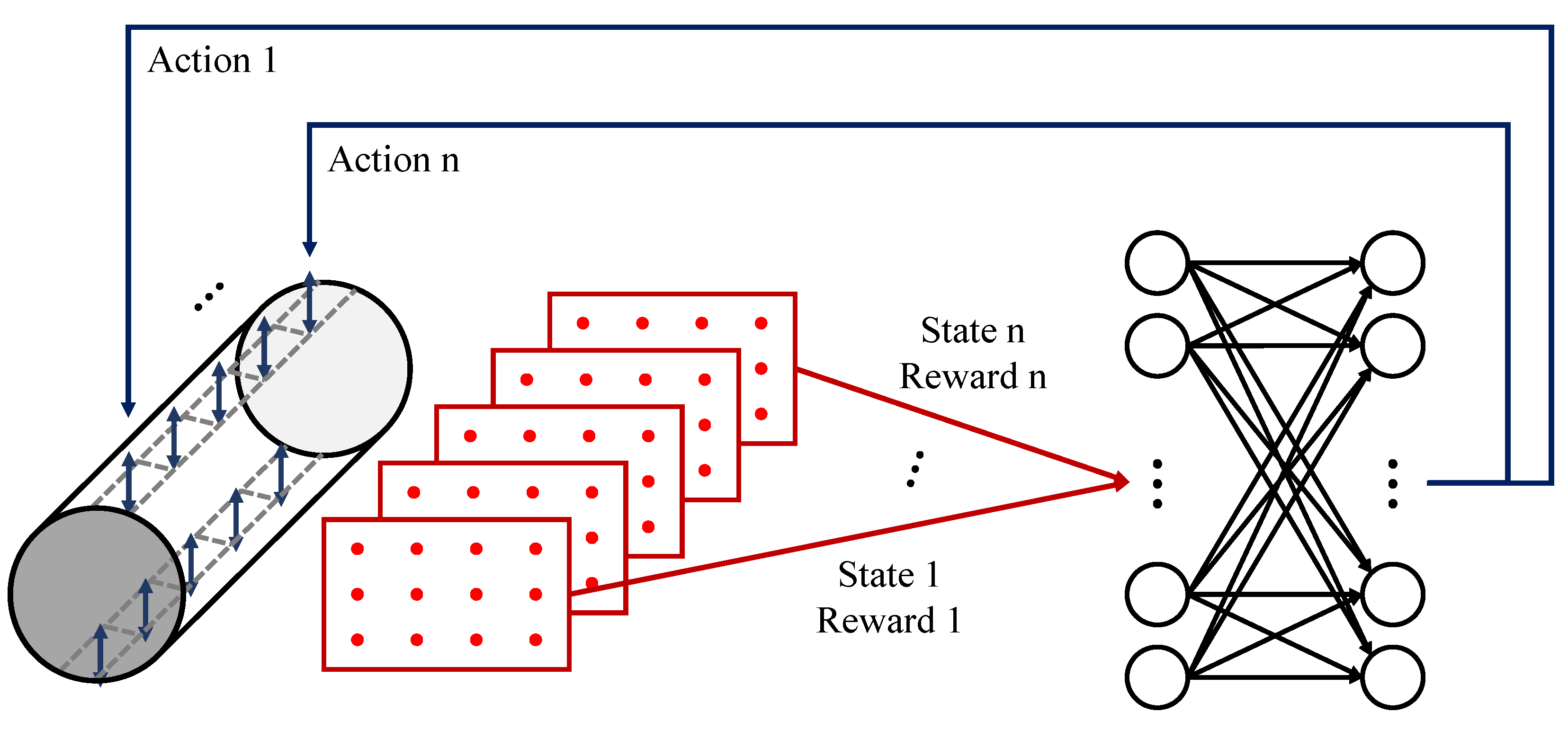
MARL (Section 3.2) is another approach to expand DRL-based flow control methods to three-dimensional configurations by assigning agents along the spanwise direction [64,65], as illustrated in Figure 4. The main advantage of MARL is its ability to significantly reduce training costs by dividing the total action space required for an entire three-dimensional domain among multiple agents.

Suárez et al. [65] employed MARL for flow control of a three-dimensional cylinder over a range of $Re=100$ to 400 to achieve drag reduction. They distributed multiple DRL agents to control the zero-net-mass-flux jets located along the spanwise direction of the cylinder and obtained drag reductions of 21% and 16.5% at $Re=300$ and $Re=400$, respectively.

More recently, Suárez et al. [64] also reported an attempt to apply MARL to turbulent flow over a cylinder at $Re=3900$, corresponding to the subcritical flow regime. The main idea of their study is similar to that of Suárez et al. [65], involving the distribution of multiple agents in the spanwise direction to control zero-net-mass-flux jets independently. Their method achieved an 8% drag reduction in a three-dimensional turbulent flow regime.

Studies addressing the practicality of control methods have been conducted considering POMDP (Section 3.3) by solely using sensor information on the surface of an object, as it is not practical to measure the entire flow field with sensor arrays in real applications.

Wang et al. [74] implemented a control method for the wake behind a three-dimensional cylinder at $Re$ = 10,000, using only sparse surface pressure probes instead of a sensor array in the wake. Their main idea is that the agent collects data from the recent 30 time steps to include the history of observations and actions, which are essential for POMDP. In their study, a DRL agent utilizing surface pressure sensors achieved similar performance to the base DRL method that uses a sensor array fully covering the wake region, in terms of reducing drag and lift fluctuations.

Similarly, Xia et al. [76] suggested a control method for the wake behind a two-dimensional square cylinder in laminar regimes using partial surface pressure measurements. They augmented the state by including current and past observations and actions, addressing the POMDP problem, and were able to achieve drag reduction performance similar to that of using near-wake sensors.

4.2. Control of Biological Systems

One of the promising research directions that leverages DRL in more complex and realistic scenarios involves controlling the biological motion of living organisms. The ability of DRL to handle highly nonlinear data facilitates the characterization of the intricate behavior dynamics of living organisms, which were challenging to define analytically.

Verma et al. [59] investigated the energy-saving swimming dynamics of a school of fish. Unlike individual fish, the movement of each fish within a school is adjusted in response to the motions of others to optimize energy use. However, the mechanisms governing such interactions have not been well understood due to the complexity of modeling the intricate swimming patterns analytically. Instead, the authors acquired an energy-efficient swimming model by training the fish school to minimize energy consumption using DRL. The trained policy was then analyzed to examine the formation and harnessing of vortical structures within the school, elucidating how these mechanisms contribute to overall energy efficiency.

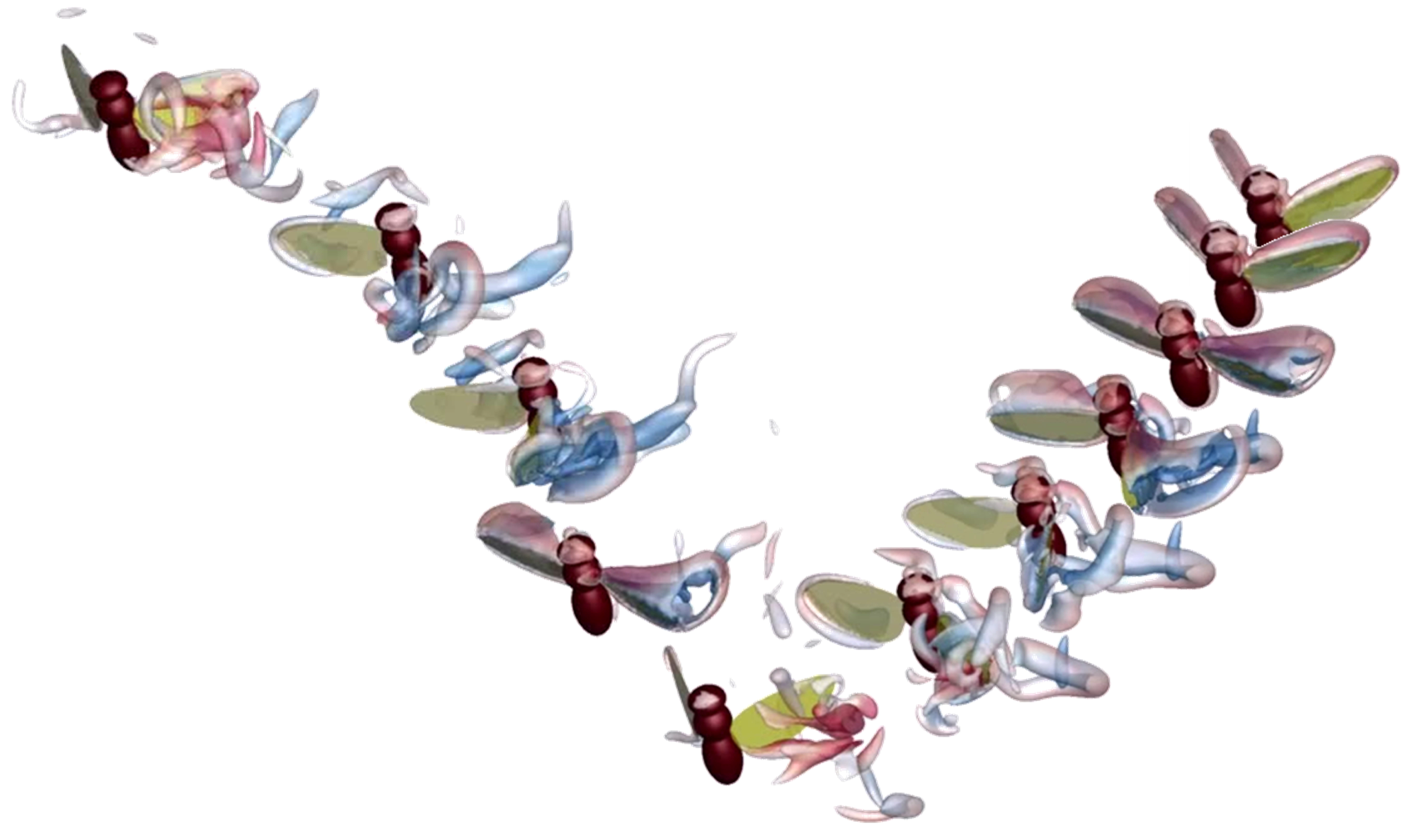
Hong et al. [83] controlled a flexible-winged flyer, approximately the size of a fruit fly, using DRL. A fluid-structure interaction simulation was incorporated to solve the complicated dynamics of the flyer accurately (see Figure 5). The position of the flyer and the surrounding flow field were used as state variables, while the frequency and amplitude of the wing movements were controlled as actions. By designing the reward function based on the distance to the destination, stable control was achieved even in complex flow environments with external disturbances such as sudden gusts of wind and raindrops.

4.3. Other Applications

DRL-based flow control methods have also been actively developed for various other applications in fluid mechanics, including drag reduction in turbulent channel flow [78,79] and airfoils [67], Rayleigh–Bénard convection [66], and optimal control of a wind farm [90].

For example, DRL-based control strategies for drag reduction in turbulent channel flow have been developed [78,79]. Sonoda et al. [79] achieved a 37% drag reduction by adapting the blowing or suction of normal velocity at the wall, using velocity fluctuations observed near the wall as the state. Guastoni et al. [78] further developed the control method by arranging DRL agents in a grid covering the bottom wall of the channel.

Additionally, a DRL-based control method for drag reduction of a NACA airfoil using synthetic jets, a strategy similar to those used for controlling cylinder wakes, was developed by Wang et al. [67]. In their study, a drag reduction of 27.0% and a lift enhancement of 27.7% were achieved after applying the flow control.

Vignon et al. [66] employed MARL to control Rayleigh–Bénard convection in a domain bounded by adiabatic walls on the top and the bottom. The control objective was to improve heat exchange performance, represented as a decrease in Nusselt number, by controlling the lower wall temperature. They successfully developed the control method with MARL by distributing the agents to multiple control segments of the lower wall, whereas the single-agent DRL failed to obtain an effective control policy.

5. Shape Optimization

Another area that has been actively studied using DRL is shape optimization. Numerous studies have focused on aerodynamic shape optimization [25,26,27,28,29,30,31,68,80,81], while other applications in shape optimization have also been reported [60,69,70].

5.1. Aerodynamic Shape Optimization

Aerodynamic shape optimization has primarily been conducted to enhance aerodynamic performance such as reducing drag or improving lift. DRL-based optimization is frequently integrated with numerical simulations. However, optimization utilizing CFD becomes computationally expensive as the Reynolds number increases due to the complexity and nonlinearity of the fluid motions. As a result, many studies have focused on using low-fidelity models or on flows at relatively low Reynolds numbers.

Viquerat et al. [25] introduced a direct shape optimization method using DRL and CFD to determine the optimal two-dimensional shape of an airfoil that maximizes the lift-to-drag ratio. The shape was represented by a set of Bézier curves defined by multiple control points. The DRL agent controls the position and the local curvature of each control point. Consequently, without prior knowledge, the DRL network generated an airfoil-like shape that enhances the lift-to-drag ratio. A single-step DRL approach was employed to generate the optimal shape from the initial state in a single attempt. However, the study was limited to relatively low Reynolds numbers.

Recently, transfer learning has been widely used to address issues related to computational cost. Bhola et al. [28] conducted a study on airfoil shape optimization to minimize drag at high Reynolds numbers using transfer learning. The method employed a multi-fidelity approach integrating potential flow and RANS simulations. The airfoil shapes were parameterized using Bézier curves, defined by six control points and the leading-edge radius. Initially, the network was trained with low-fidelity data from potential flow simulations. The trained weights were then fine-tuned using high-fidelity data from RANS simulations, as illustrated in Figure 6. By utilizing the multi-fidelity transfer learning approach, computational costs were significantly reduced compared to retraining from scratch. Similarly, Yan et al. [80] applied multi-fidelity transfer learning to enhance the lift-to-drag ratio in the aerodynamic shape optimization of missile control surfaces. The study integrated semi-empirical methods with CFD, resulting in significant computational cost savings.

Another significant issue in DRL-based shape optimization is that the optimization process must be restarted from scratch for different problems, such as different target geometries or flow conditions. Such a requirement adversely affects the generalization performance of shape optimization using DRL. Therefore, methods that can be applied to various problem scenarios have recently been developed.

Li et al. [29] utilized DRL and a DNN-based surrogate model to develop a policy for reducing the aerodynamic drag of supercritical airfoils. The surrogate model, trained with CFD data, was used for performance evaluation to reduce computational costs. The agent was trained to execute actions based on features of the wall Mach number distribution to enhance the generalizability across different airfoils and flow conditions. In another study, Kim et al. [30] developed a multi-condition multi-objective optimization method and applied it to airfoil shape optimization. The method not only accommodated multi-objective problems (i.e., lift and lift-to-drag ratio) but also addressed various conditions (i.e., Reynolds and Mach numbers). The developed method was able to obtain the optimal shape without the need for retraining the optimization process from scratch, even if conditions or objectives change (see Figure 7).

5.2. Other Applications

In addition to research focusing on aerodynamic shape optimization, other applications of DRL-based shape optimization have also been studied. Keramati et al. [69] conducted a study to optimize the fin shape at solid–fluid interfaces of a heat exchanger to maximize the heat transfer-to-pressure drop ratio. The fin geometry was represented by a set of Bézier curves, and the training of DRL was performed by gradually adjusting the positions of control points. As a result, the overall heat transfer of the optimized shape was improved and the pressure drop was reduced compared to the rectangular reference geometry.

Ma et al. [60] optimized a rocket nozzle to improve the thrust using DRL and a surrogate model parameterized by a convolutional neural network (CNN). The surrogate model was initially developed to predict the flow field based on geometric information and was used for performance evaluation with reduced computational cost. The nozzle shape was parameterized by basis spline (B-spline) curves, where the positions of the control points were optimized during the training. The DRL agent was able to produce an optimized nozzle shape that resembles the theoretically driven solution exhibiting improved thrust compared to the baseline model.

6. Automation of Computational Fluid Dynamics

Developing accurate, reliable, and efficient CFD methods, such as constructing high-quality meshes, designing precise turbulence models, and formulating effective numerical schemes, is a highly expert-intensive task. Given that the Navier–Stokes equations do not have a priori solutions, even experts must rely on iterative and experience-dependent approaches to develop effective techniques based on physical intuition. Recently, DRL has been explored as an automatic development tool for CFD methods, utilizing its trial-and-error learning approach to replace the heuristic methods traditionally dependent on expert intervention. This section reviews recent research on the automation of CFD using DRL, focusing on mesh generation, turbulence modeling, and numerical schemes.

6.1. Mesh Generation

Mesh generation is a foundational step in conducting CFD, but it remains one of the most time-consuming and labor-intensive tasks. Despite advancements in automation methods, developing techniques that achieve both the diversity of applications and the high quality required for accuracy solely through human intuition is challenging. Manual interventions are often required to obtain optimal meshes iteratively for each new configuration. Recently, DRL, with its ability to dynamically adapt to changing state variables for maximum cumulative reward, has emerged as a promising solution to the generality and optimality challenges inherent in traditional automation techniques.

Pan et al. [77] employed DRL to automatically generate high-quality quadrilateral meshes within two-dimensional domains. In their approach, the current boundary configuration was defined as the state, and creating a quadrilateral element constituted the action. Upon executing the action, the subsequent state was updated to reflect the new boundary formed after the element was added. By defining partially observable boundaries based on specified vertices, rather than the entire geometry, the method was able to achieve generalizability across various geometries.

While the previous study focused on automating mesh generation from a geometrical perspective, Foucart et al. [61] and Dzanic et al. [71] optimized mesh resolution to balance simulation accuracy and computational cost. The method employed DRL to explore adaptive mesh refinement strategies, dynamically adjusting the resolution in critical regions. The trained DRL agent evaluated each cell to determine whether further refinement or coarsening is necessary, defining such decisions as actions. By utilizing a POMDP formulation, the agent effectively learned from the partial information surrounding the cell where the action was performed.

Kim et al. [58] developed a method to generate optimal meshes in terms of both geometric quality and resolution. The study targeted RANS simulations of flow through a blade passage. Given various blade profiles and flow conditions, the DRL agents generated meshes and conducted CFD simulations, optimizing the accuracy and cost of the solutions within a multi-objective framework. The novelty of the study lies in the utilization of a single-step DRL approach, enabling the acquisition of the optimal mesh and solution in a single attempt based on the given configuration. Consequently, a grid-converged solution was obtained in a non-iterative manner, eliminating the need for repetitive CFD processes required for grid convergence tests, thereby automating the CFD workflow with great efficiency.

The study strategically separated the training phase into two steps to alleviate the computational burden of data acquisition with CFD. The approach allowed for the segmentation of the overall action space dimension. The initial phase, as outlined in the work of Kim et al. [57], focused on optimizing the geometric quality of the mesh independently of CFD simulations. The agents were trained to improve quality metrics, such as the min-max ratio of determinants of the Jacobian matrices and cell skewness, for randomly assigned blade profiles in each training episode. Figure 8 illustrates an example of the training process for a specific blade profile, clearly demonstrating the capability of DRL to generate higher-quality meshes. It is important to note that the actual training was conducted with randomly assigned blade profiles to ensure generalizability.

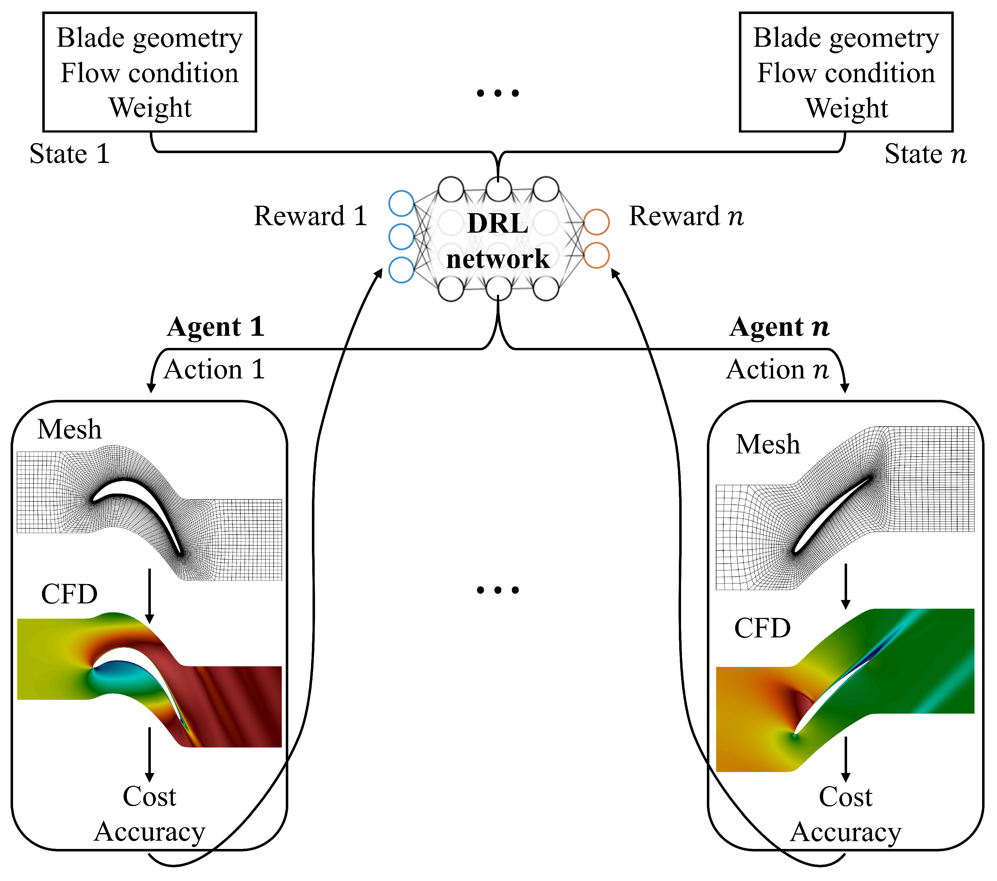
In the subsequent phase, the pre-trained network for geometric quality was refined to define the optimal resolution by incorporating CFD simulations. To further accelerate data acquisition, the study employed the MARL framework. As illustrated in Figure 9, multiple agents simultaneously performed tasks of mesh generation and CFD analysis in parallel, continuously providing data to the main network to optimize the accuracy and cost of the solutions. The trained network was able to non-iteratively produce grid-converged solutions at a desired computational expense for various blade configurations, effectively capturing complex physical phenomena such as shock waves and flow separation.

6.2. Turbulence Modeling

In the field of data-driven turbulence modeling, there have been many attempts to develop turbulence models using supervised learning methods. Regarding turbulence models for LES, for example, the models with supervised learning have shown great possibilities showing partial improvement over algebraic turbulence models for canonical turbulent flows, such as homogeneous isotropic turbulence [91,92,93,94,95,96], turbulent channel flow [97,98,99], and flow over a circular cylinder [100]. However, since labeled data are required for supervised learning, a higher fidelity simulation (i.e., DNS) needs to be conducted a priori to obtain the unresolved flow quantities as labeled target data, which limits the practicality.

Therefore, DRL frameworks for turbulence closure modeling have been newly proposed by controlling the unresolved closure term as an action and using the errors in the statistical properties of the reference simulation as a reward. Novati et al. [86] integrated MARL with an LES solver by deploying DRL agents at sampling points distributed throughout a computational domain of homogeneous isotropic turbulence, and achieved good generalization performance across Reynolds numbers and grid sizes. In the study of Kurz et al. [72], a similar DRL-based closure model for LES of homogeneous isotropic turbulence, in which a CNN is used for the policy network instead of fully connected layers, was developed.

Kim et al. [84] applied a similar DRL approach to turbulence modeling for LES in turbulent channel flow. In their method, the DRL produces the subgrid-scale stress for wall-bounded turbulent flow during the simulation, based on a reward designed to reduce errors in the statistical properties (see Figure 10). They reported better performance of the developed DRL model compared to algebraic subgrid-scale models in various turbulence statistics.

Bae and Koumoutsakos [87] further developed the MARL approach for wall modeling for LES. Agents are distributed at the walls of the channel, and their actions are given as the magnitude of the modeled wall shear stress, while the reward is defined to minimize the error between the modeled and the true mean wall shear stress. The developed wall model successfully generalized to extremely high Reynolds numbers, exhibiting similar off-wall velocity profiles to those from fully resolved simulations.

In the field of RANS closure modeling, Fuchs et al. [73] introduced a DRL-based model by adding a source term into the transport equation of the Spalart–Allmaras RANS model, controlled by a DRL algorithm. A reward is defined to reduce the error between the velocity field using the developed RANS model and the time-averaged LES field. Their model is trained for turbulent jet flow at $Re$ = 10,000 and successfully generalized to $Re$ = 15,000.

6.3. Numerical Scheme

Feng et al. [62] optimized the numerical scheme for compressible flow simulations to dynamically balance dispersion and dissipation according to flow evolution. To analyze compressible flow, significant gradients, such as shock waves, necessitate numerical dissipation to stabilize the simulation. However, most existing methods apply dissipation non-selectively across scales, leading to physical inconsistencies. The study aimed to develop a physically consistent numerical scheme by dynamically adjusting the scheme to different subgrid-scale types: genuine (discontinuities and interfaces) and non-genuine (fluctuations and turbulence). Specifically, tunable parameters of the fifth-order targeted essentially non-oscillatory scheme (TENO5), which determine the dissipation and dispersion terms, were optimized using DRL. The current flow variables are defined as the state, and the parameters of the TENO5 scheme are optimized as the action. As a result, the trained network was able to capture small-scale dynamics while maintaining the stability of the simulation. Although there is currently limited literature in this area, DRL has the potential to develop a self-adaptive scheme across different flow configurations, automating the definition of appropriate numerical schemes in the CFD process.

7. Concluding Remarks

Recent advancements in the application of deep reinforcement learning (DRL) to fluid dynamics problems have been comprehensively reviewed. The present review not only synthesizes current research but also highlights strategies employed to overcome challenges in applying DRL to complex, real-world engineering problems, including data efficiency, turbulence, and partial observability. Specifically, the use of transfer learning, multi-agent reinforcement learning, and the partially observable Markov decision process in DRL-based fluid dynamics research is explained. The reviewed literature is categorized by application: flow control and shape optimization, which are the main fields where DRL is currently applied, as well as automation of computational fluid dynamics, an emerging and promising field for advancing the efficiency and reliability of numerical analysis. Despite such progress, ongoing research is essential toward the ultimate objective of training control, optimization, and automation policies capable of addressing intricate geometries and highly turbulent regimes and generalizing such capabilities across diverse configurations. Continued innovation in algorithm development, data handling methods, and computational techniques will be crucial. Exploring advancements to address related problems in different fields, such as computer vision, robotics, and natural language processing, can offer valuable insights.