Abstract
This paper introduces innovative approaches to enhance and develop one-equation RANS models using gene-expression programming. Two distinct strategies are explored: overcoming the limitations of the Boussinesq hypothesis and formulating a novel one-equation turbulence model that can accurately predict a wide range of turbulent wall-bounded flows. A comparative analysis of these strategies highlights their potential for advancing RANS modeling capabilities. The study employs a single-case CFD-driven machine learning framework, demonstrating that machine-informed models significantly improve predictive accuracy, especially when baseline RANS predictions diverge from established benchmarks. Using existing training data, symbolic regression provides valuable insights into the underlying physics by eliminating ineffective strategies. This highlights the broader significance of machine learning beyond developing turbulence closures for specific cases.
1. Introduction
The Reynolds-averaged Navier–Stokes (RANS) turbulence closure is widely preferred in industrial settings primarily because it demands significantly less computational resources compared to high-fidelity (Hi-Fi) simulations like large-eddy simulation (LES) and hybrid RANS/LES. Nevertheless, RANS often falls short in its predictive accuracy when dealing with complex geometries and flow dynamics [1,2,3]. This constraint predominantly arises from the assumptions underlying the modeling of the Reynolds stress tensor and the turbulence model employed to close the RANS equations. To properly model the Reynolds stresses, the commonly used Boussinesq hypothesis assumes a linear relationship between the Reynolds stress tensor and the deviatoric part of the mean strain rate . Although this hypothesis works in many situations, it can produce unsatisfactory predictions for various turbulent flows [4]. Boussinesq postulated that the momentum transfer caused by turbulent eddies could be modeled using eddy viscosity [5]. Several eddy-viscosity models (EVMs) exist, which can be classified according to the number of transport equations solved to compute the eddy viscosity.
Historically, a diverse array of turbulence models have been proposed, spanning from rudimentary algebraic models such as Prandtl’s mixing length hypothesis [6] to comprehensive stress-transport models like the Launder–Reece–Rodi model [7]. Nonetheless, when applied to practical technical challenges, these turbulence models’ increased complexity and heightened computational demands do not always correlate with a marked enhancement in solution quality. A comprehensive introduction to several widely adopted turbulence models can be found in Ref. [8]. The efficacy and predictive accuracy of numerous models, including the Baldwin–Lomax, Baldwin–Barth, Spalart–Allmaras (SA) [9], standard , , and the SST [10] have been extensively detailed in several studies [11,12].
The SA model is a standard RANS closure for aerodynamic applications, particularly within the industrial sector, owing to its robustness and reliability. However, the SA turbulence model has exhibited discrepancies compared to the model [13]. It tends to be less accurate in capturing certain turbulent flow features, especially near walls or regions with adverse pressure gradients. Another limitation of the one-equation model is the inability to predict both wall-bounded and free-shear flows consistently [14]. Therefore, the academic and industrial communities are strongly committed to enhancing the predictive accuracy of the SA turbulence model, particularly in the context of validating aerodynamic designs within the aerospace sector.
Recent progress in data science has reinvigorated scientific research focused on turbulence modeling. Various data analysis instruments have been introduced with the advancement of high-performance computing, enabling more complex simulations and state-of-the-art experimental tools that provide comprehensive datasets. These instruments can derive essential physical insights from the data to enhance RANS modeling [15,16,17,18]. Nevertheless, although data have historically been instrumental in refining model coefficients and assessing the model uncertainty [18], the capacity to exploit this expansive dataset remains predominantly underutilized. Therefore, incorporating data-driven techniques into turbulence modeling consistently maintains its relevance.
Within the domain of turbulence modeling, machine learning (ML) has achieved notable advancements [16]. Various ML techniques have been employed to enhance the predictive capacity of conventional RANS models. These methodologies include the calibration of model parameters via the Bayesian approach [19], the incorporation of a neural network-informed correction component for the turbulence production term [20], and the integration of a spatially varying correction field using field inversion and Gaussian process techniques [21], among others. Beyond merely introducing corrections to pre-existing model parameters, significant efforts have been directed toward developing new Reynolds stress closures through physics-informed machine learning. A prominent area of focus has been on refining the Boussinesq hypothesis. Wang et al. [22] utilized a random forest method to train functions representing Reynolds stress discrepancies. Ling et al. [23] employed a deep neural network to train the Reynolds stress tensor while ensuring the conservation of Galilean invariance. However, integrating the resulting neural networks into standard RANS solvers presents several challenges, and many of the proposed corrections often lack clear physical interpretability.
The adoption of ML in developing turbulence models has significantly increased, yet challenges remain in training and applying these models in engineering contexts. A key issue is the predominant focus on training techniques that model the Reynolds stress tensor using a static, fixed database of high-fidelity data. This approach, often referred to as frozen training, has been effectively implemented across various ML platforms, including deep neural networks [23,24,25,26], Gaussian processes [20], random forests [22], adaptive boosting [27], sparse symbolic regression [28], and evolutionary algorithms [29]. However, separating the learning and prediction stages frequently results in discrepancies between a priori and a posteriori evaluations. The inherent differences between RANS modeling and high-fidelity data are often neglected [16,30,31], raising concerns about the efficacy of model development approaches that prioritize accurate modeling of using high-fidelity data for predicting accurate mean flow dynamics.
To address this limitation, this research uses an innovative framework known as CFD-driven training, where the fitness or effectiveness of proposed models is directly assessed through RANS calculations [32,33]. This approach builds upon the gene expression programming (GEP) method [34]. However, instead of relying on an algebraic function for assessment, it performs RANS calculations, potentially offering a more integrative and comprehensive evaluation of the model’s capabilities. This method’s flexibility in defining the cost function is a notable distinction from other data-driven approaches. Rather than limiting the fitness evaluation to match Reynolds stresses with high-fidelity data, this method allows for any flow feature from the CFD results to define the cost function. This adaptability is invaluable, particularly when access to extensive training data is restricted.
This study aims to analyze the most efficient ways to optimize one equation of the SA model by comparing two main strategies. These results will form the basis for future multi-case, multi-objective optimization endeavors. The first strategy involves modifying the linear Boussinesq hypothesis to capture and model Reynolds stress anisotropy more accurately, thereby improving predictive accuracy. The second strategy focuses on developing an enhanced one-equation turbulence model that better represents turbulence production and destruction within the flow field. The SA model is then employed in its standard version or with modifications designed to improve prediction capabilities. These modifications include adjusting coefficients in the production and destruction terms of the original SA equation or creating a new eddy-viscosity turbulence equation, denoted as Coupled Spalart–Allmaras (CSA), following an approach similar to Fares and Schröder [14]. The CSA presents a new robust and general one-equation model capable of accurately predicting a broad spectrum of fundamental turbulent flows by mitigating the dependency on the wall distance.
Four wall-bounded flows from the NASA challenge validation cases—namely, the flat plate, channel, jet, and wall-mounted hump (accessible at [35]) are used for the training process. These flows exhibit complex dynamics, such as significant wall curvature, pronounced flow separation, and exceptionally high Reynolds numbers, which are crucial during the model’s optimization phase. The flow cases are considered individually in single-case CFD-driven training, followed by an analysis of the derived model expressions. Machine learning leverages existing training data to uncover the underlying physics by discarding ineffective strategies. Specifically, this research demonstrates the need to modify the SA equation, leading to a new turbulence model to enhance the numerical predictions in alignment with experimental data. This demonstrates the broader impact of machine learning beyond merely developing turbulence closures for specific scenarios.
The structure of this paper is as follows. Section 2 presents the two distinct methodologies to improve RANS calculations’ accuracy. The first approach focuses on developing RANS closures capable of enhancing the Boussinesq assumption by modeling the anisotropy of the Reynolds stress tensor, as detailed in Section 2.1. Section 2.1.1 introduces RANS and the Boussinesq hypothesis. Subsequently, Section 2.1.2 explains the method used to model the extra anisotropy. The second approach involves deriving a novel one-equation turbulence model, as discussed in Section 2.2. The baseline SA model and the derivation of the new one-equation model are introduced in Section 2.2.1 and Section 2.2.2, respectively. Continuing with the methodology section, an explanation of the CFD-driven framework is provided in Section 2.3. Subsequently, Section 3 examines the numerical results compared with the available experimental data. Finally, the paper concludes with a summary in Section 4.
2. Methodology
2.1. Beyond the Boussinesq Hypothesis: Modeling Reynolds Stress Anisotropy
2.1.1. RANS Equations and the Boussinesq Hypothesis
The RANS equations are derived from the general Navier–Stokes equations, representing the averaged motion of fluid flow. In these equations, the mean value is separated from the fluctuating component, which accounts for turbulence under various flow conditions [36]. For a steady-state incompressible Newtonian fluid, the RANS equations in Einstein notation and Cartesian coordinates are expressed as
where the left-hand side represents the change in mean momentum due to convection by the mean flow. This change is balanced by the mean body force, isotropic stress from the mean pressure field, viscous stresses, and the Reynolds stress resulting from velocity fluctuations. The nonlinearity of the convective term necessitates additional modeling to close the RANS equations, leading to various turbulence models. The Boussinesq hypothesis posits that the Reynolds stress tensor is proportional to the traceless mean strain rate tensor, , expressed as
where is the eddy viscosity, and , with (the overbars denoting the mean variable are omitted for simplicity in the following).
Boussinesq suggested that the momentum transfer by turbulent eddies could be represented using eddy viscosity [5]. Various EVMs have since been developed, differing in the number of transport equations used to calculate the eddy viscosity. This study employs the SA model, as detailed in Section 2.2.1.
2.1.2. Development of Anisotropy Models
Given the limitations of the Boussinesq hypothesis, turbulence closures such as explicit algebraic stress models (EASMs) offer improvements by incorporating additional anisotropic stress terms, , into the Reynolds stress tensor:
EASM-like closures are expressed in non-dimensionalized form as
where the non-dimensionalized anisotropic stress tensor combines tensor bases and scalar invariants [37]. The models are derived using symbolic regression through GEP [34], determining coefficients from training datasets. Three tensor bases and two invariants are used for the two-dimensional flow [37]. The tensor basis and the invariants used in the present study are expressed as
Here, and are derived from the non-dimensionalized strain rate tensor and rotation rate tensor , with the vorticity tensor . Inspired by the SA model with quadratic constitutive relation (QCR) [38], the turbulence time scale is computed from the velocity gradient tensor’s magnitude as follows:
The dimensionalized extra anisotropic stress tensor is obtained from the modeled non-dimensionalized as follows:
and the Reynolds stress tensor equation becomes
2.2. The Enhanced One-Equation Turbulence Model
2.2.1. Spalart–Allmaras One-Equation Model: Baseline and GEP-Optimized Version
The development of the new model is grounded in the widely utilized SA model [39], which formulates eddy-viscosity turbulence using a single transport equation for the eddy-viscosity variable, . The eddy viscosity is linearly related to the Reynolds stresses, , consistent with the Boussinesq assumption in Equation (2). Unlike two-equation models, the SA model neglects the turbulence kinetic energy, k. The transport equation for the modified eddy viscosity, , in its incompressible form is
where the production term depends on
with the vorticity magnitude computed from the vorticity tensor . The value of the coefficients and further explanations can be found in Ref. [9].
The diffusion term in the SA model includes both a classical diffusion operator and a non-conservative term to reflect aerodynamic flow behavior [9]. One major source of numerical mispredictions in the SA model arises from the production and destruction terms [40,41,42]. Therefore, the diffusion terms in Equation (9) remain unchanged.
An alternative approach involves optimizing the standard SA model by modifying the production and destruction coefficients using GEP. The resulting model, termed SA+PD, is expressed as
with the coefficients and being functions of the invariants and from Equation (5).
2.2.2. Derivation of the New One-Equation Turbulence Model
The derivation of the new one-equation turbulence model begins with the well-established two-equation model by Wilcox [8]:
where is the eddy viscosity, and the turbulence production term is
An equation for can be derived using the eddy-viscosity definition in Equation (13) [10,43]:
Substituting and retaining the original model’s diffusion term, we obtain
To address the destruction term, noting that in a one-equation model, the turbulence length scale is equivalent to the wall distance, d, we scale the turbulence kinetic energy as , leading to [44]. Thus, the destruction term becomes , similar to the original SA model. For the production term, is used as a parameter to non-dimensionalize the strain rate tensor and is reconstructed using the velocity gradient tensor magnitude , where is given by Equation (6).
Utilizing definitions from the original SA model [9],
the new one-equation turbulence model for is
To reduce the dependency on wall distance, we implement a blending function, , designed to be 1 in the LES region (away from the wall) and 0 near the wall (RANS region) [45]:
Thus, the destruction term is modified as follows:
where from Wilcox [8] and is the magnitude of the strain rate tensor. This ensures the destruction term’s value is never smaller than the original, but it can increase away from the wall in high-strain regions to balance the production term.
Finally, the coefficients from the original SA model have been tested and found effective, resulting in the new Coupled Spalart–Allmaras (CSA) model:
2.3. Training Frameworks: CFD-Driven Method
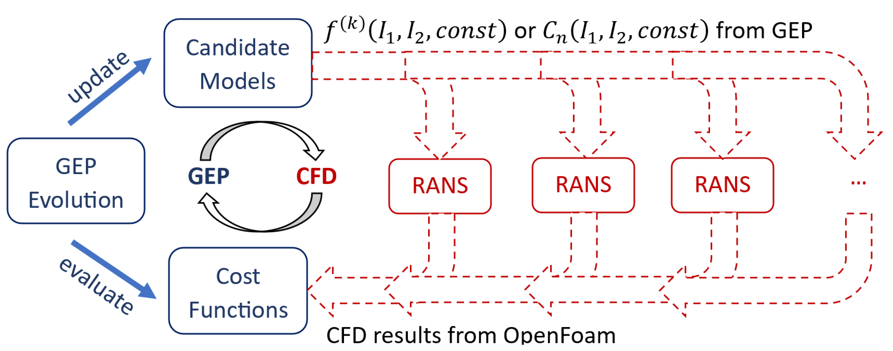
The present research employs an innovative methodology that integrates CFD simulations into model training iterations, referred to as CFD-driven training, as depicted in Figure 1 [32,33]. This framework consists of two main segments. The first segment involves the CFD solver, where OpenFOAM V7 [46] performs RANS computations. The second segment is the ML module, specifically using GEP due to its proven effectiveness in addressing challenges related to turbulence closures, heat flux, and transition models [32,33,47,48,49,50,51].
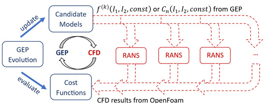
Figure 1.
CFD-driven training scheme [32].
The pioneering work by Weatheritt and Sandberg [34] introduced using GEP to enhance the Boussinesq approximation within RANS. The training process starts with generating a set of random candidate models, known as individuals, derived from a predefined set of mathematical symbols. These symbols include mathematical operations (e.g., addition, subtraction, multiplication), variables, and constants (random or predefined). During each generation of the training process, a subset of individuals evolves, affecting their evolutionary path. These selected individuals are then integrated into RANS calculations to evaluate a cost function which measures the mean square deviation between numerical predictions and the “ground truth” (experimental data). Models that better represent the training data exhibit lower cost values and are more likely to be selected for the next generation. The cost function formulation is dependent on the training framework and specific conditions.
Following the first strategy detailed in Section 2.1.2, the GEP training begins with an initial set of EASMs, represented as . Throughout the optimization, the tensor bases remain fixed, while the coefficients , functions of , are determined. These functions are generated randomly, with each candidate model containing four genes representing unique coefficients for . The expression length for the coefficient function is mainly determined by the gene’s head length and the truncation level of its expression tree. In this study, the head length is set to 5, the maximum size of the expression tree is limited to 12, and the population size is set to 400. The total number of generations is 100. For more details on the configuration parameters of GEP, refer to the following references: [34,52].
The anisotropy of Reynolds stresses is modeled using both the SA model (Equation (9)) and the CSA model (Equation (20)) as turbulence closure equations. The CSA turbulence model allows for the simultaneous optimization of Reynolds stresses and the production term, similar to the approach used for the two-equation SST model [32,34]. The same GEP settings are applied for the optimization process, aiming to find the optimal values for the coefficients and in the production and destruction terms, as detailed in the SA+PD model (Equation (10)).
3. Results and Discussion
A comprehensive optimization of RANS turbulence models was pursued to improve the predictive accuracy of RANS for a set of fundamental wall-bounded flows. Using existing experimental data, machine learning provides valuable insights into the underlying physics by highlighting the best strategies for improving one-equation RANS predictions. Specifically, four NASA challenge validation cases (accessible at [35]) are tested and employed to perform the training process:
- 2DZP: 2D Zero Pressure Gradient Flat Plate (in Section 3.1);
- 2DFDC: 2D Fully Developed Channel Flow at a High Reynolds Number (in Section 3.2);
- 2DWMH: 2D NASA Wall-Mounted Hump with Flow Separation (in Section 3.3);
- ASJ: Axisymmetric Subsonic Jet (in Section 3.4).
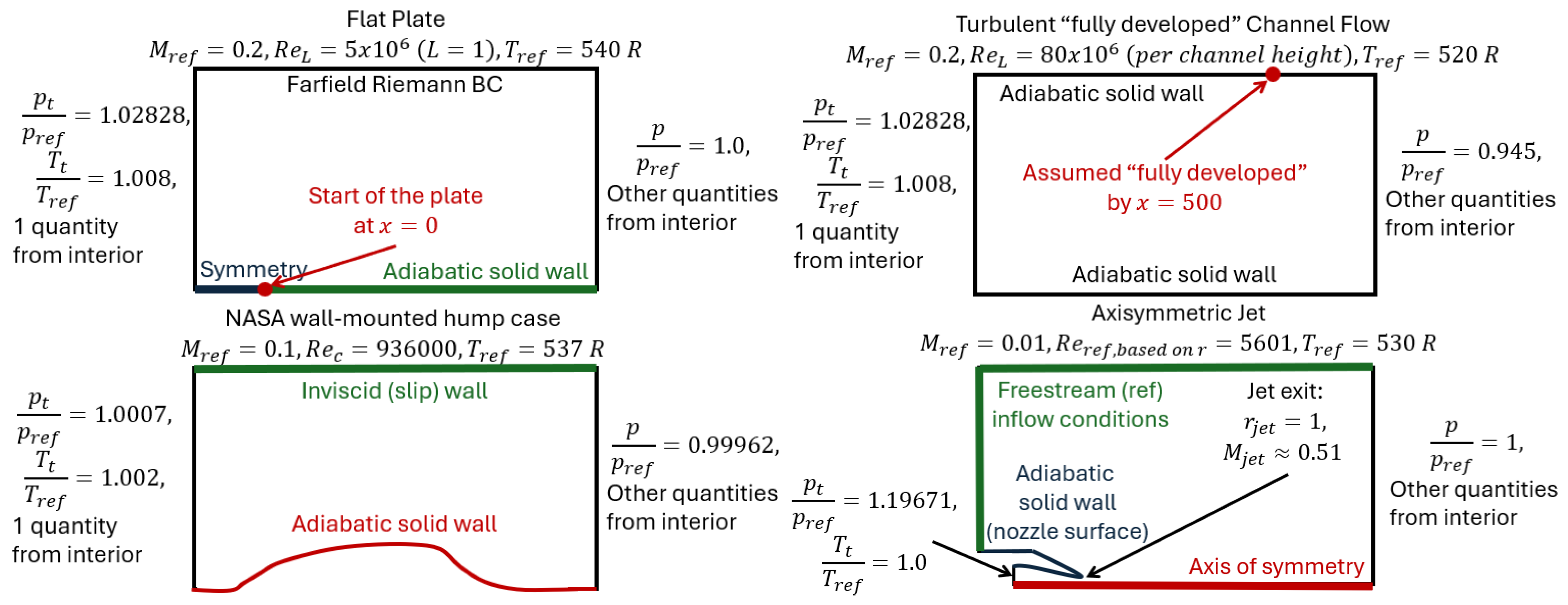
The computational domains and boundary conditions are schematically illustrated in Figure 2. The employed meshes were downloaded from the NASA website to minimize numerical errors and ensure numerical results consistent with those already available.
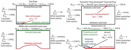
Figure 2.
Introduction to NASA validation cases (inspired by [35]).
Specific profiles of relevant quantities regarding the cost functions have been delineated for each case. For instance, the streamwise friction coefficient and the velocity at relative to the distance from the wall are the focal points for the flat plate case. The velocity at against the distance from the wall informed the channel flow training. The jet case training was oriented by the streamwise velocity and shear stress profiles at the ratios . For the wall-mounted hump case, the cost function has integrated the friction and pressure coefficients along the hump’s surface, in conjunction with the streamwise velocity profiles preceding and succeeding the separation bubble, specifically at axial positions , , and .
For the RANS simulations, the rhoPimpleFoam solver is explicitly used for the compressible jet, while the other cases utilize simpleFoam within the OpenFOAM framework [46]. The numerical approach is described by following the OpenFOAM parameter nomenclature, ensuring ease of understanding and reproducibility. The numerical schemes are tailored for a steady-state analysis. The gradient computations default to a Gaussian linear approach, with a specific cell-limited modification applied to the velocity gradient to enhance numerical stability. The divergence schemes are meticulously selected for different variables: a bounded linear upwind scheme is used for velocity fluxes, ensuring accuracy while preventing numerical oscillations; an upwind scheme is adopted for the turbulence model variable, , favoring stability; and a standard Gauss linear scheme is applied for the effective viscosity multiplied by the deviatoric tensor of the velocity gradient, aiming for a balance between accuracy and stability. The Laplacian terms employ a Gauss linear corrected scheme to improve accuracy by correcting for mesh non-orthogonality. Linear interpolation is used as the default for intermediate values, and the surface normal gradients are corrected to account for mesh irregularities, ensuring that the simulation results are both accurate and reliable.
Five simulation results are compared with the experimental data in the present work. The methodologies presented in Section 2 are thus tested.
- SA+: Standard SA turbulence model in Equation (9) and optimizing by modeling the Reynolds extra stress anisotropy , as introduced in Section 2.1 in Equations (3) and (4). GEP provides the coefficients that multiply the basis tensors for modeling the tensor .
- SA+PD: The classical Boussinesq assumption in Equation (2) is applied with an optimized version of the SA turbulence model in Equation (10). Indeed, the original production and destruction coefficients of the SA equation, and , respectively, are substituted with and , found through GEP optimization.
- CSA+: The modeled is included in the new turbulence production term in Equation (20) by noticing that . This allows for optimization of both the anisotropy tensor and the turbulence production term with the same three coefficients: , and . The employed production term in the one-equation model thus becomesThe new production term has the advantage that changes in are reflected in itself, not just in the Boussinesq assumption. In this way, double optimization is possible while modeling the anisotropy of the Reynolds stress (as detailed in Section 2.1.2).
3.1. 2D Zero Pressure Gradient Flat Plate
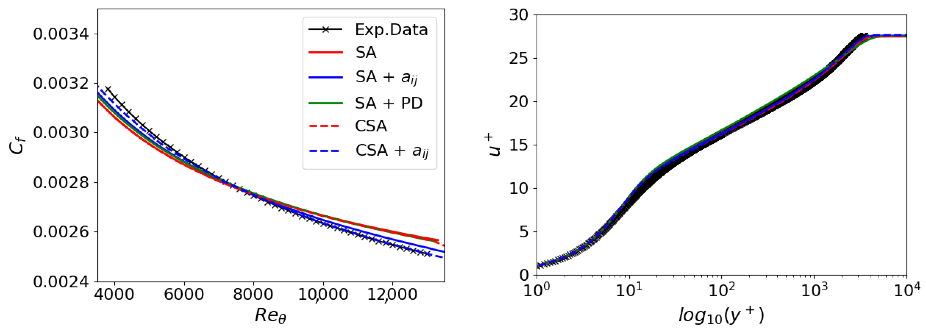
Figure 3 shows the friction coefficient across the flat plate and the velocity at relative to the distance from the wall. These numerical outcomes are juxtaposed with data from White et al. [53]. The original model SA yields predictions congruent with the theoretical assessments concerning the velocity relative to the wall’s distance. However, it shows either reduced or increased values for the friction coefficient for values of less than or larger than 7500. Nevertheless, the numerical predictions correctly represent the wall’s velocity law. All models, except for the CSA + , display some inconsistencies in the friction coefficient prediction while they agree with the log-law velocity profile.
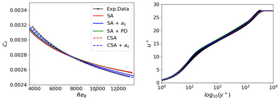
Figure 3.
2DZP: Friction coefficient on the left and velocity profile (law of the wall) on the right.
Since the SA + PD models do not improve upon the original SA model, optimizing the original SA model’s coefficients for the flat plate test case is impossible. Indeed, they have been optimized for this case. Contrarily, the inclusion of SA + notably enhances prediction, particularly in the downstream region of the flat plate. However, this adjustment does not yield significant improvements in the upstream section. Therefore, a new formulation of the one-equation turbulence model is needed, and the CSA model proves helpful. Its original version is stable and consistent with the SA model, but simultaneously, it allows for more accurate optimization through GEP. This capability should be attributed to the fact that optimizing the anisotropy of Reynolds stresses also impacts the production term. In essence, a kind of double optimization with a single extension is possible.
Table 1 summarizes the expressions found by the GEP training. All numbers in the tables are rounded to the third decimal place. As detailed in Equations (4) and (5), the tensors associated with the functions , , and are , , and , respectively.

Table 1.
2DZP: GEP training expressions.
3.2. 2D Fully Developed Channel Flow at High Reynolds Number
The velocity profile for channel flow at the position is illustrated in Figure 4. All models align closely with the theoretical results from White et al. [53]. All the models effectively capture the vertical stratification of the viscous layer, logarithmic, and turbulent regions, even under exceedingly high Reynolds numbers. These results demonstrate how the hybrid RANS/LES blending function included in the destruction term of the CSA model (see Equation (20)) does not compromise the preservation of the law of the wall, as the velocity profile is well captured. Table 2 summarizes the expressions found by the GEP training for the channel flow.
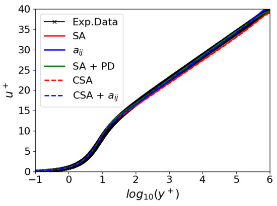
Figure 4.
2DFDC: Law of the wall.

Table 2.
2DFDC: GEP training expressions.
3.3. 2D NASA Wall-Mounted Hump-Separated Flow
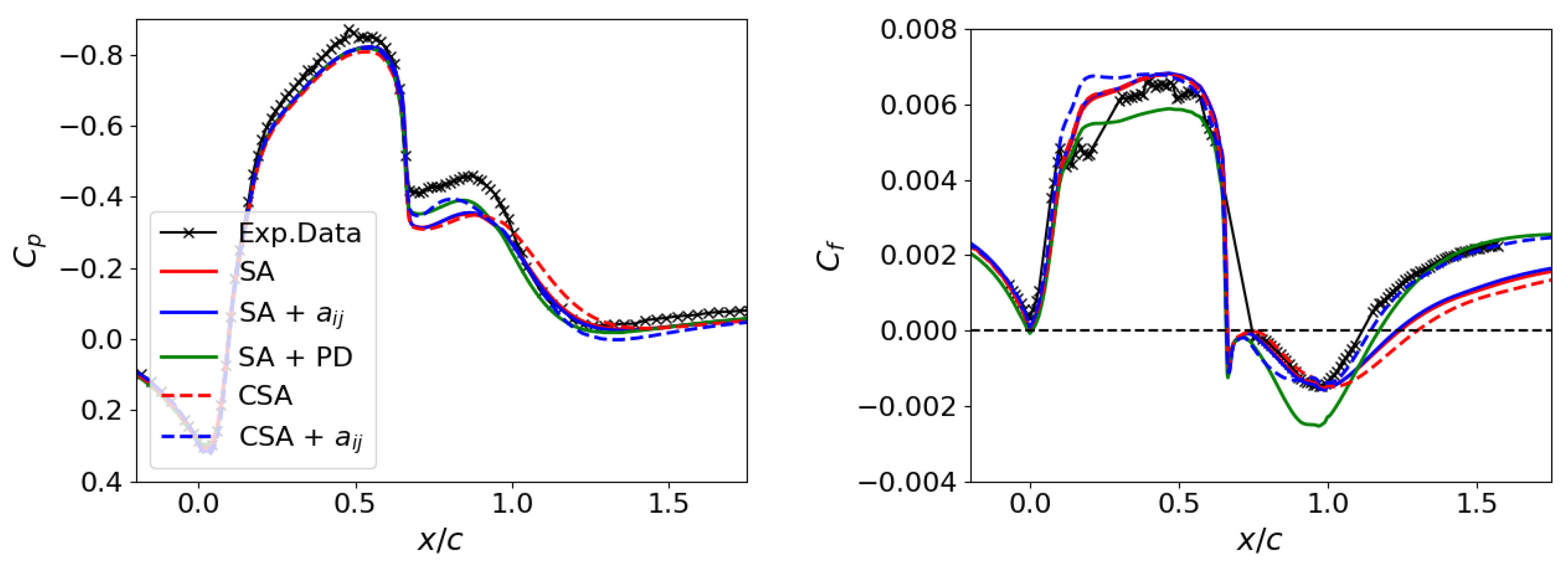
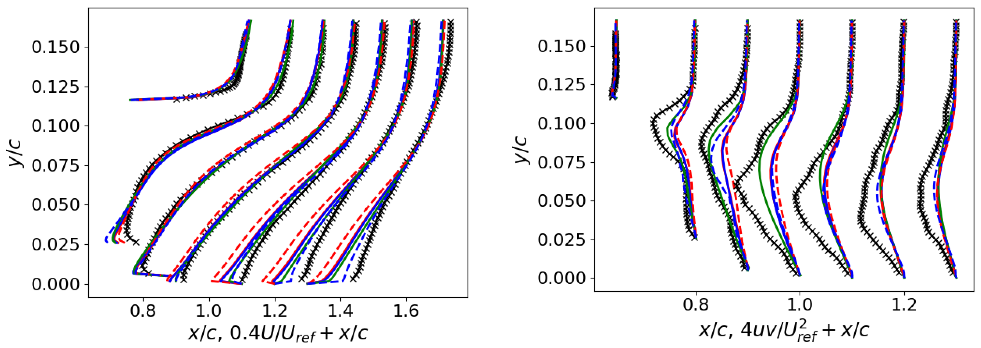
Figure 5 and Figure 6 display the juxtaposition of numerical results with experimental data from Seifert et al. [54] for the hump case. The pressure and friction coefficients along the hump’s surface are illustrated in Figure 5. The reattachment point, and consequently, the size of the separation bubble, is identified where . Significant discrepancies manifest proximal to and succeeding the separation bubble. The SA model generally underestimates both coefficients post-bubble, similar to the deviation for the flat plate in Section 3.1. The distinction lies in the magnitude of the friction coefficient discrepancies for the hump, which are more pronounced than those for the flat plate.
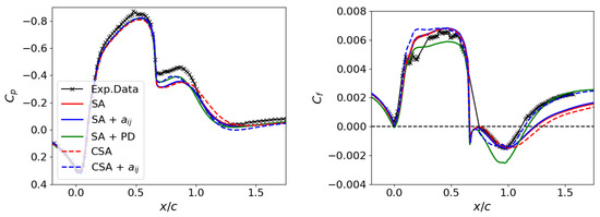
Figure 5.
2DWMH: Friction coefficient on the left and pressure coefficient on the right.
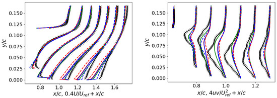
Figure 6.
2DWMH: Velocity profiles on the left and Reynolds stress profiles on the right (refer to Figure 5 for the legend).
Figure 6 shows the velocity and shear stress profiles at various locations. Examining the velocity profiles, the deviation intensifies as one moves closer to the hump’s surface. In shear stress profiles, pronounced differences emerge near the separation bubble. Even though they were not incorporated as constituents of the cost functions during model development, they have been more accurately captured by the CSA + and SA + PD models.
The CSA model slightly diverges from the SA model but aligns with the SST model presented in Ref. [4]. All the trained models, excluding SA + , enhance the numerical predictions. Notably, the CSA + model yields outcomes remarkably congruent with the reference data and provides one of the best predictions obtained from a one-equation model [4]. Therefore, as investigated in the SA + model, modifying Reynolds stresses alone by modeling the anisotropic tensor is insufficient to capture the reattachment point correctly. Instead, training the production term (see Equation (21)) in the CSA + model is crucial to improve the prediction of the separation bubble size.
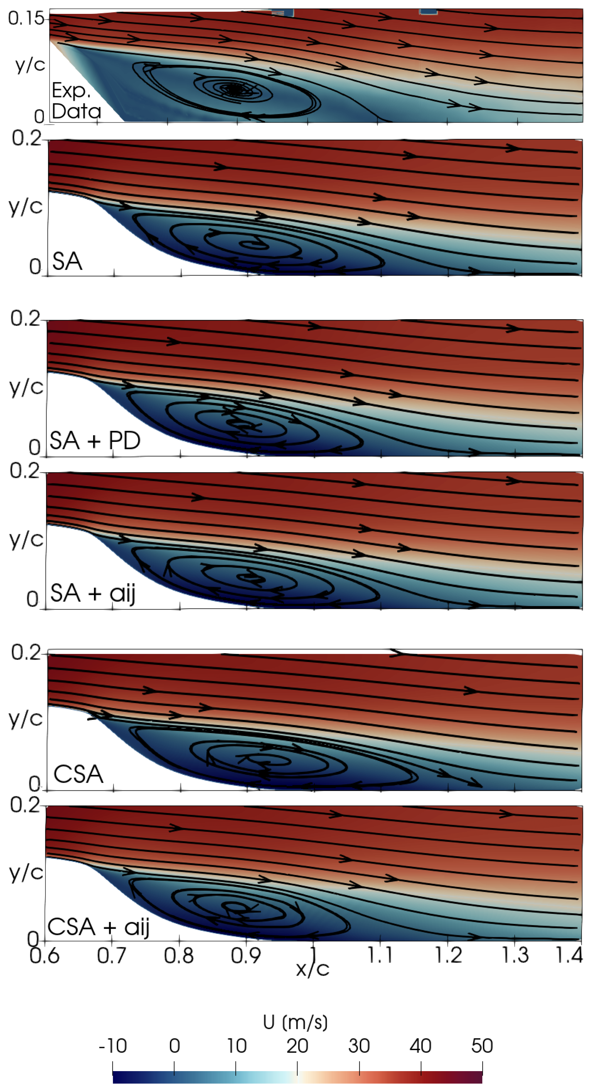
Figure 7 delineates the performance of the trained models through flow field contours; in particular, the x-velocity is plotted to analyze the flow physics in more detail. Streamlines are employed to elucidate the separation bubbles, comparing experimental data with numerical results. As depicted in Figure 5 and Figure 7, the reattachment point approximates in the experiments, in contrast to the observed with the SA model. Flow fields derived from CSA + and SA + PD exhibit remarkable similarities, and these models relocate the reattachment to , while the SA + model does not reduce it. The trained models then offer a flow representation at the hump’s down ramp that closely depicts the experimental observations.

Figure 7.
2DWMH: Velocity contour plots.
The expressions derived from the GEP training for the hump case are summarized in Table 3 and are subject to detailed analysis herein. Figure 8 depicts the distribution of the function for the CSA + model because, as discussed by Fang et al. [32], the coefficient is the most influential term in Equation (4). In addition, Figure 8 illustrates the coefficients and for the SA + PD model. The function exhibits oscillations within the range of to in the separation zone, indicating unsteadiness in the simulation. Regarding the SA + PD model, the coefficients and are observed to maintain constant values, approximately and , respectively. The coefficient exceeds the original model’s corresponding , and the destruction term reaches values an order of magnitude larger than the original value . This indicates that the original SA model is not well suited to deal with separated flow because the destruction term vanishes, scaling with . This represents the motivation for the modified destruction term in the CSA model.

Table 3.
2DWMH: GEP training expressions.
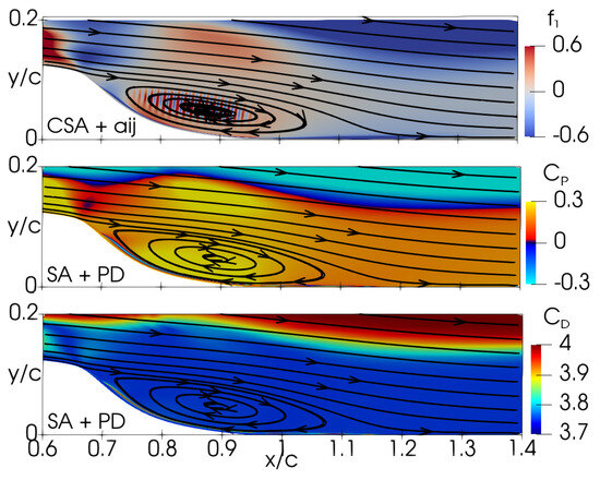
Figure 8.
2DWMH: Distribution of GEP expressions for the CSA + and SA + PD models. Top to bottom: , , and .
The GEP expressions are formulated as functions of the two invariants and , as detailed in Section 2.1.2 and Table 3. This relationship is depicted in Figure 9. The axes are limited to unity because the invariants are non-dimensionalized with the magnitude of the velocity gradient tensor. When the vorticity magnitude surpasses the strain rate magnitude (), is positive; conversely, it is negative in the opposite scenario. The two values exhibit high similarity in the separation zone, oscillating between negative and positive magnitudes. A similar but less pronounced trend is evident in the plot of the coefficient. In contrast, reaches a maximum value of 4 and decreases with increasing invariants. Therefore, an increase in the production term is needed when vorticity exceeds the strain rate and vice versa. Simultaneously, the destruction term should be reduced.

Figure 9.
2DWMH: GEP expressions as function of the invariants.
3.4. Axisymmetric Subsonic Jet
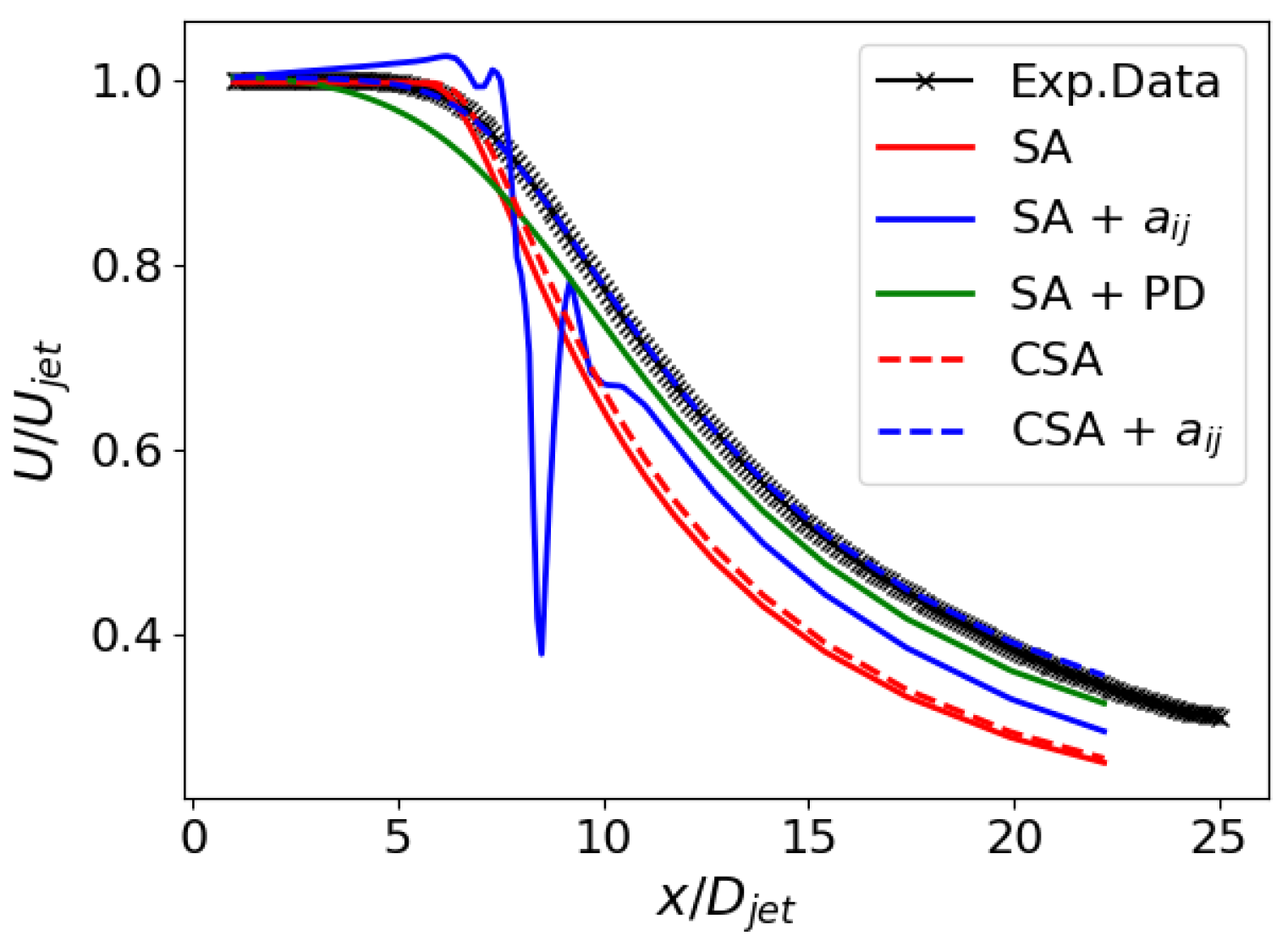
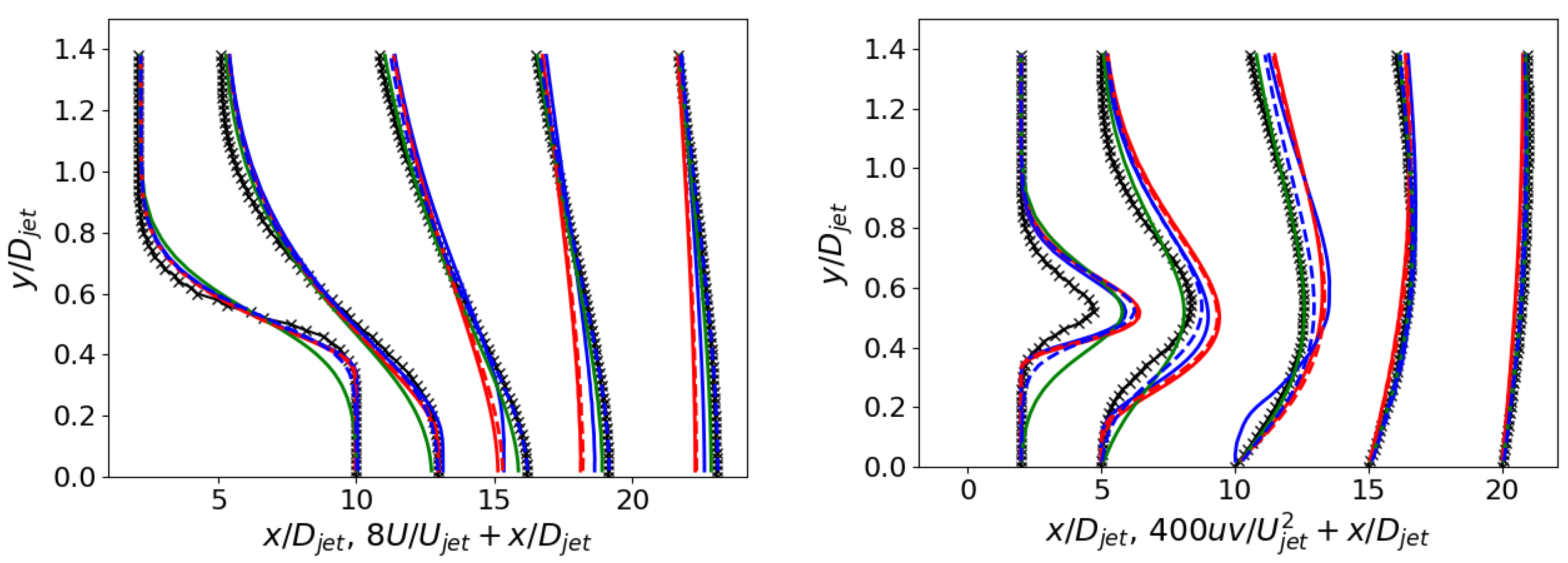
Figure 10 and Figure 11 show the jet case’s velocity and shear stress profiles along the jet axis and at various locations. Both models, CSA + and SA + PD, exhibit comparable performance, curtailing diffusion and refining the mean flow and second-moment profiles. Considering the shear stress profiles, while the advancements are not as pronounced as observed in the velocity profiles, they are impressive, given that RANS primarily centers on mean flow parameters. Instead, the SA + model is numerically unstable and presents only marginal enhancements, even in this flow case.
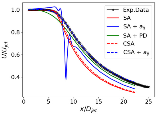
Figure 10.
ASJ: Velocity profiles along the jet axis.
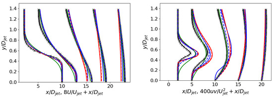
Figure 11.
ASJ: Velocity profiles on the left and Reynolds stress profiles on the right (refer to Figure 10 for the legend).
In addition, in the jet case, the original SA destruction term in Equation (9) is not very pertinent, given the dependence on the wall distance. The CSA model using the hybrid RANS/LES blending function seems to point in the right direction for enhancing the numerical results.
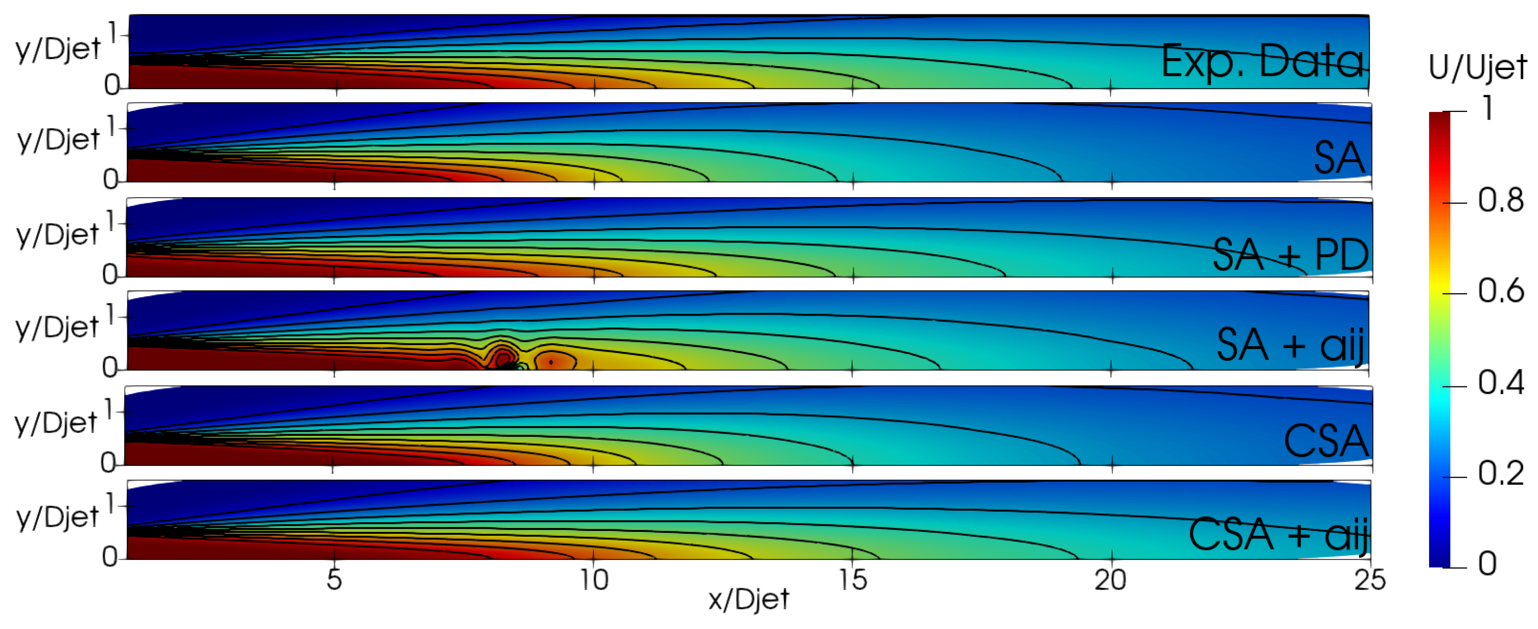
Figure 12 delineates the performance of the trained models through flow field contours. The SA + model fails to achieve convergence and exhibits undesirable non-stationary effects. Further investigation is warranted to elucidate the underlying mechanisms contributing to these observed phenomena. The flow fields derived from CSA + and SA + PD exhibit remarkable similarities, constricting the jet radius and prolonging the jet length relative to the baseline simulation. These trained models display a smaller jet radius compared to the baseline. The velocity decreases slower along the centerline, which can be attributed to reduced diffusion [32]. It is important to note that modification consistently affects the entire jet region, rather than providing varying corrections in the laminar (), transition (), and fully turbulent () regions. For all the trained models, a less accurate streamwise velocity prediction in the transition region is noticed in Figure 11. However, this is expected since the new model was designed to emphasize turbulence mixing using a cost function based on velocity profiles in the fully turbulent region.
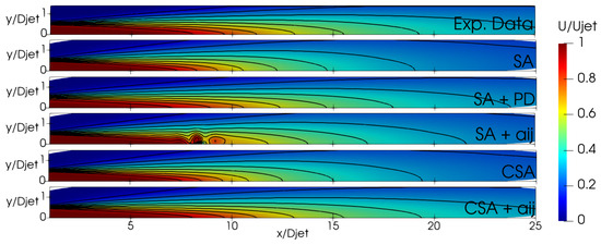
Figure 12.
ASJ: Normalized velocity contour plots.
Table 4 summarizes the expressions found by the GEP training. Figure 13 and Figure 14 illustrate the function for the CSA + model and the coefficients and for the SA + PD model. The function maintains a constant value of in the jet region. The coefficients and hold steady at approximately and , respectively. Notably, the coefficient is slightly lower than the original model’s corresponding . Variations are observed in the vicinity of the jet axis. Given its dependency on the two invariants, the value of the function remains predominantly negligible, except in instances characterized by elevated vorticity and significant strain-rate stress. and are almost always positive unless is at least one order of magnitude bigger than . Their values remain nearly constant in the jet region, at approximately 0.1 and 0.195, respectively. This implies that the trained model consistently requires less production than the original model.

Table 4.
ASJ: GEP training expressions.

Figure 13.
ASJ: Distribution of GEP expressions for the CSA + and SA + PD models. Top to bottom: , , and .

Figure 14.
ASJ: GEP expressions as functions of the invariants.
4. Conclusions and Outlook
This work explores enhancing RANS modeling capabilities using two methodologies discussed in Section 2. The first approach involves utilizing the standard SA model to close the RANS equations and improving predictive accuracy by modifying the linear Boussinesq hypothesis to capture and model Reynolds stress anisotropy more effectively. The second approach builds upon the Boussinesq hypothesis and attempts to augment RANS modeling performance by creating an enhanced one-equation turbulence model designed to enhance turbulence production and destruction. It is important to emphasize that the current work aims not to develop a final model but to understand the requirements for improving the SA model.
Section 3 examines the numerical results compared with the available experimental data. Four wall-bounded flows of the NASA challenge validation cases (flat plate, channel, wall-mounted hump, and jet) are employed to perform the training process. The flow cases are considered individually, and the derived model expressions are subsequently analyzed. Five simulation results are compared with the experimental data in the present work: SA, SA + , SA + PD, CSA, and CSA + . Using existing experimental data, machine learning provides valuable insights into the underlying physics by highlighting the best strategies for improving one-equation RANS predictions.
The SA + model consistently fails to surpass the baseline and, in some instances, demonstrates instability. Therefore, modifying Reynolds stresses alone by modeling the anisotropic tensor is insufficient for the present investigations to improve the RANS capability using the SA turbulence model.
The CSA model performs comparably to SA, yet its formulation enables effective coupling with anisotropic formulations for Reynolds stresses in the CSA + model. In addition, the modified destruction term does not vanish away from the walls, which makes the model potentially more suitable for separated flows. The new production term has the advantage that changes in are reflected in itself, not just in the Boussinesq assumption. In this way, double optimization is possible while modeling the anisotropy of the Reynolds stress. Similarly, in the SA + PD model, modifications to the production and destruction terms in the SA model allow for effective optimization of model performance. Indeed, the analysis of the expressions found by GEP revealed the necessity for an effective change in the production term depending on the vorticity or the magnitude of the strain stress. This explains the favorable results obtained by the CSA + and SA + PD models and the lack of improvement observed with the SA + model.
Since the CSA + and SA + PD models demonstrate superior accuracy, two ways for optimizing the SA model are suggested: either by refining the coefficients in the original formulation or by adopting a new version that incorporates the Reynolds stress tensor in the production term, modeling its anisotropy. In addition, optimizing the baseline CSA model by training its coefficients holds the potential for further improvement.
Finally, a primary motivation for further studies will be to enhance the generalizability of data-driven one-equation turbulence models, focusing on optimizing their performance simultaneously across a range of flow conditions and different configurations during the training process. Multi-objective optimization is necessary and is part of the ongoing work. The goal of further studies will be to enhance the generalizability of the identified models through machine learning by concurrently training the algorithm on the four cases discussed. The generalized model will then be validated on different test cases to assess its applicability. In addition, training more complex and challenging configurations will be investigated by considering the available computational resources. The universality of the results and usefulness of the investigated approaches will be evaluated for future extension to more complex flow cases (3D, transonic, supersonic) using different software to further validate the considerations expressed in the current manuscript.
Author Contributions
Conceptualization, T.D.F. and Y.F.; methodology, T.D.F. and Y.F.; software, T.D.F. and Y.F.; validation, E.T., R.D.S. and M.K.; formal analysis, Y.F. and R.D.S.; investigation, T.D.F.; resources, R.D.S. and M.K.; data curation, T.D.F.; writing—original draft preparation, T.D.F.; writing—review and editing, Y.F. and E.T.; visualization, T.D.F.; supervision, R.D.S. and M.K.; project administration, E.T.; funding acquisition, T.D.F. and M.K. All authors have read and agreed to the published version of the manuscript.
Funding
This research was funded by the German Academic Exchange Service (DAAD), program ID 57694189.
Data Availability Statement
The datasets presented in this article are not readily available because the data are part of an ongoing study. Requests to access the datasets should be directed to the correspondence author.
Conflicts of Interest
The authors declare that this study received funding from the German Academic Exchange Service (DAAD). The funder was not involved in the study design, collection, analysis, interpretation of data, the writing of this article or the decision to submit it for publication.
References
- Werner, M.; Schütte, A.; Weiss, S. Turbulence Model Effects on the Prediction of Transonic Vortex Interaction on a Multi-Swept Delta Wing. In Proceedings of the AIAA SCITECH Forum, San Diego, CA, USA, 3–7 January 2022. [Google Scholar] [CrossRef]
- Werner, M.; Rein, M.; Richter, K.; Weiss, S. Experimental and numerical analysis of the aerodynamics and vortex interactions on multi-swept delta wings. CEAS Aeronaut. J. 2023, 14, 927–938. [Google Scholar] [CrossRef]
- Di Fabbio, T.; Tangermann, E.; Klein, M. Investigation of transonic aerodynamics on a triple-delta wing in side slip conditions. CEAS Aeronaut. J. 2022, 13, 453–470. [Google Scholar] [CrossRef]
- Rumsey, C.; Coleman, G. NASA Symposium on Turbulence Modeling: Roadblocks, and the Potential for Machine Learning, 2022. Available online: https://ntrs.nasa.gov/citations/20220015595 (accessed on 1 August 2024).
- Boussinesq, J.V. Essai sur la Théorie des Eaux Courantes; Impr. Nationale: Ithaca, NY, USA, 1877. [Google Scholar]
- Prandtl, L. Über die ausgebildete turbulenz (investigations on turbulent flow). Z. Angew. Math. Mech. 1925, 5, 136–139. [Google Scholar] [CrossRef]
- Launder, B.E.; Reece, G.J.; Rodi, W. Progress in the development of a Reynolds-stress turbulence closure. J. Fluid Mech. 1975, 68, 537–566. [Google Scholar] [CrossRef]
- Wilcox, D.C. Turbulence Modeling for CFD; DCW Industries: La Canada, CA, USA, 1998; Volume 2. [Google Scholar]
- Spalart, P.; Allmaras, S. A one-equation turbulence model for aerodynamic flows. In Proceedings of the 30th Aerospace Sciences Meeting and Exhibit, Reno, NV, USA, 6–9 January 1992; p. 439. [Google Scholar]
- Menter, F. Zonal two equation kw turbulence models for aerodynamic flows. In Proceedings of the 23rd Fluid Dynamics, Plasmadynamics, and Lasers Conference, Orlando, FL, USA, 6–9 July 1993; p. 2906. [Google Scholar]
- Shur, M.; Strelets, M.; Zajkov, L.; Gulyaev, A.; Kozlov, V.; Sekundov, A. Comparative numerical testing of one-and two-equation turbulence models for flows with separation and reattachment. In Proceedings of the 33rd Aerospace Sciences Meeting and Exhibit, Reno, NV, USA, 9–12 January 1995; p. 863. [Google Scholar]
- Wilcox, D.C. Reassessment of the scale-determining equation for advanced turbulence models. AIAA J. 1988, 26, 1299–1310. [Google Scholar] [CrossRef]
- Menter, F.R. Two-equation eddy-viscosity turbulence models for engineering applications. AIAA J. 1994, 32, 1598–1605. [Google Scholar] [CrossRef]
- Fares, E.; Schröder, W. A general one-equation turbulence model for free shear and wall-bounded flows. Flow Turbul. Combust. 2005, 73, 187–215. [Google Scholar] [CrossRef]
- Duraisamy, K.; Spalart, P.R.; Rumsey, C.L. Status, Emerging Ideas and Future Directions of Turbulence Modeling Research in Aeronautics. 2017. Available online: https://ntrs.nasa.gov/citations/20170011477 (accessed on 1 August 2024).
- Duraisamy, K.; Iaccarino, G.; Xiao, H. Annual Review of Fluid Mechanics Turbulence Modeling in the Age of Data. Annu. Rev. Fluid Mech 2019, 51, 357–377. [Google Scholar] [CrossRef]
- Durbin, P.A. Some recent developments in turbulence closure modeling. Annu. Rev. Fluid Mech. 2018, 50, 77–103. [Google Scholar] [CrossRef]
- Brunton, S.L.; Noack, B.R.; Koumoutsakos, P. Machine learning for fluid mechanics. Annu. Rev. Fluid Mech. 2020, 52, 477–508. [Google Scholar] [CrossRef]
- Edeling, W.N.; Cinnella, P.; Dwight, R.P.; Bijl, H. Bayesian estimates of parameter variability in the k-ϵ turbulence model. J. Comput. Phys. 2014, 258, 73–94. [Google Scholar] [CrossRef]
- Zhang, Z.J.; Duraisamy, K. Machine learning methods for data-driven turbulence modeling. In Proceedings of the 22nd AIAA Computational Fluid Dynamics Conference, Dallas, TX, USA, 22–26 June 2015; p. 2460. [Google Scholar]
- Parish, E.J.; Duraisamy, K. A paradigm for data-driven predictive modeling using field inversion and machine learning. J. Comput. Phys. 2016, 305, 758–774. [Google Scholar] [CrossRef]
- Wang, J.X.; Wu, J.L.; Xiao, H. Physics-informed machine learning approach for reconstructing Reynolds stress modeling discrepancies based on DNS data. Phys. Rev. Fluids 2017, 2, 034603. [Google Scholar] [CrossRef]
- Ling, J.; Kurzawski, A.; Templeton, J. Reynolds averaged turbulence modelling using deep neural networks with embedded invariance. J. Fluid Mech. 2016, 807, 155–166. [Google Scholar] [CrossRef]
- Zhang, Z.; Ye, S.; Yin, B.; Song, X.; Wang, Y.; Huang, C.; Chen, Y. A semi-implicit discrepancy model of Reynolds stress in a higher-order tensor basis framework for Reynolds-averaged Navier–Stokes simulations. AIP Adv. 2021, 11, 045025. [Google Scholar] [CrossRef]
- Ling, J.; Jones, R.; Templeton, J. Machine learning strategies for systems with invariance properties. J. Comput. Phys. 2016, 318, 22–35. [Google Scholar] [CrossRef]
- Zhang, Z.; Song, X.D.; Ye, S.R.; Wang, Y.W.; Huang, C.G.; An, Y.R.; Chen, Y.S. Application of deep learning method to Reynolds stress models of channel flow based on reduced-order modeling of DNS data. J. Hydrodyn. 2019, 31, 58–65. [Google Scholar] [CrossRef]
- Singh, A.P.; Duraisamy, K.; Zhang, Z.J. Augmentation of turbulence models using field inversion and machine learning. In Proceedings of the 55th AIAA Aerospace Sciences Meeting, Grapevine, TX, USA, 9–13 January 2017; p. 0993. [Google Scholar]
- Schmelzer, M.; Dwight, R.P.; Cinnella, P. Discovery of algebraic Reynolds-stress models using sparse symbolic regression. Flow Turbul. Combust. 2020, 104, 579–603. [Google Scholar] [CrossRef]
- Akolekar, H.D.; Weatheritt, J.; Hutchins, N.; Sandberg, R.D.; Laskowski, G.; Michelassi, V. Development and use of machine-learnt algebraic Reynolds stress models for enhanced prediction of wake mixing in low-pressure turbines. J. Turbomach. 2019, 141, 041010. [Google Scholar] [CrossRef]
- Thompson, R.L.; Sampaio, L.E.B.; de Bragança Alves, F.A.; Thais, L.; Mompean, G. A methodology to evaluate statistical errors in DNS data of plane channel flows. Comput. Fluids 2016, 130, 1–7. [Google Scholar] [CrossRef]
- Poroseva, S.V.; Colmenares F, J.D.; Murman, S.M. On the accuracy of RANS simulations with DNS data. Phys. Fluids 2016, 28, 115102. [Google Scholar] [CrossRef] [PubMed]
- Fang, Y.; Zhao, Y.; Waschkowski, F.; Ooi, A.S.; Sandberg, R.D. Toward More General Turbulence Models via Multicase Computational-Fluid-Dynamics-Driven Training. AIAA J. 2023, 61, 2100–2115. [Google Scholar] [CrossRef]
- Zhao, Y.; Akolekar, H.D.; Weatheritt, J.; Michelassi, V.; Sandberg, R.D. RANS turbulence model development using CFD-driven machine learning. J. Comput. Phys. 2020, 411, 109413. [Google Scholar] [CrossRef]
- Weatheritt, J.; Sandberg, R. A novel evolutionary algorithm applied to algebraic modifications of the RANS stress–strain relationship. J. Comput. Phys. 2016, 325, 22–37. [Google Scholar] [CrossRef]
- Rumsey, C. Turbulence Modeling Resource. Available online: https://turbmodels.larc.nasa.gov (accessed on 19 July 2024).
- Reynolds, O. IV. On the dynamical theory of incompressible viscous fluids and the determination of the criterion. Philos. Trans. R. Soc. Lond. (A) 1895, 186, 123–164. [Google Scholar]
- Pope, S.B. A more general effective-viscosity hypothesis. J. Fluid Mech. 1975, 72, 331–340. [Google Scholar] [CrossRef]
- Rumsey, C.L.; Carlson, J.R.; Pulliam, T.H.; Spalart, P.R. Improvements to the Quadratic Constitutive Relation Based on NASA Juncture Flow Data. AIAA J. 2020, 58, 4374–4384. [Google Scholar] [CrossRef]
- Spalart, P.R. Strategies for turbulence modelling and simulations. Int. J. Heat Fluid Flow 2000, 21, 252–263. [Google Scholar] [CrossRef]
- Moioli, M.; Breitsamter, C.; Sørensen, K. Turbulence Modeling for Leading-Edge Vortices: An Enhancement based on Experimental Data. In Proceedings of the AIAA SciTech Forum, Orlando, FL, USA, 6–10 January 2020. [Google Scholar] [CrossRef]
- Moioli, M.; Breitsamter, C.; Sørensen, K.A. Parametric data-based turbulence modelling for vortex dominated flows. Int. J. Comput. Fluid Dyn. 2019, 33, 149–170. [Google Scholar] [CrossRef]
- Di Fabbio, T.; Rajkumar, K.; Tangermann, E.; Klein, M. Towards the understanding of vortex breakdown for improved RANS turbulence modeling. Aerosp. Sci. Technol. 2024, 146, 108973. [Google Scholar] [CrossRef]
- Baldwin, B.; Barth, T. A one-equation turbulence transport model for high Reynolds number wall-bounded flows. In Proceedings of the 29th Aerospace Sciences Meeting, Reno, NV, USA, 7–10 January 1991; p. 610. [Google Scholar]
- Bradshaw, P.; Ferriss, D.; Atwell, N. Calculation of boundary-layer development using the turbulent energy equation. J. Fluid Mech. 1967, 28, 593–616. [Google Scholar] [CrossRef]
- Spalart, P.R.; Deck, S.; Shur, M.L.; Squires, K.D.; Strelets, M.K.; Travin, A. A new version of detached-eddy simulation, resistant to ambiguous grid densities. Theor. Comput. Fluid Dyn. 2006, 20, 181–195. [Google Scholar] [CrossRef]
- Weller, H.G.; Tabor, G.; Jasak, H.; Fureby, C. A tensorial approach to computational continuum mechanics using object-oriented techniques. Comput. Phys. 1998, 12, 620–631. [Google Scholar] [CrossRef]
- Xu, X.; Waschkowski, F.; Ooi, A.S.; Sandberg, R.D. Towards robust and accurate Reynolds-averaged closures for natural convection via multi-objective CFD-driven machine learning. Int. J. Heat Mass Transf. 2022, 187, 122557. [Google Scholar] [CrossRef]
- Lav, C.; Haghiri, A.; Sandberg, R. RANS predictions of trailing-edge slot flows using heat-flux closures developed with CFD-driven machine learning. J. Glob. Power Propuls. Soc. 2021, 2021, 1–13. [Google Scholar] [CrossRef]
- Akolekar, H.D.; Waschkowski, F.; Zhao, Y.; Pacciani, R.; Sandberg, R.D. Transition modeling for low pressure turbines using computational fluid dynamics driven machine learning. Energies 2021, 14, 4680. [Google Scholar] [CrossRef]
- Wilsby, O.L.; Sandberg, R.D. Data-Driven RANS Closures for Trailing Edge Noise Predictions. In Proceedings of the 25th AIAA/CEAS Aeroacoustics Conference, Delft, The Netherlands, 20–23 May 2019; p. 2444. [Google Scholar]
- Lav, C.; Sandberg, R.D.; Philip, J. A framework to develop data-driven turbulence models for flows with organised unsteadiness. J. Comput. Phys. 2019, 383, 148–165. [Google Scholar] [CrossRef]
- Weatheritt, J.; Sandberg, R.D. The development of algebraic stress models using a novel evolutionary algorithm. Int. J. Heat Fluid Flow 2017, 68, 298–318. [Google Scholar] [CrossRef]
- White, F.M.; Majdalani, J. Viscous Fluid Flow; McGraw-Hill: New York, NY, USA, 2006; Volume 3. [Google Scholar]
- Seifert, A.; Pack, L.G. Active flow separation control on wall-mounted hump at high Reynolds numbers. AIAA J. 2002, 40, 1363–1372. [Google Scholar] [CrossRef]
Disclaimer/Publisher’s Note: The statements, opinions and data contained in all publications are solely those of the individual author(s) and contributor(s) and not of MDPI and/or the editor(s). MDPI and/or the editor(s) disclaim responsibility for any injury to people or property resulting from any ideas, methods, instructions or products referred to in the content. |
© 2024 by the authors. Licensee MDPI, Basel, Switzerland. This article is an open access article distributed under the terms and conditions of the Creative Commons Attribution (CC BY) license (https://creativecommons.org/licenses/by/4.0/).

