

Simulation on the Separation of Breast Cancer Cells within a Dual-Patterned End Microfluidic Device


Abstract
1. Introduction
2. Materials and Methods
2.1. Mathematical Method
Governing Equations
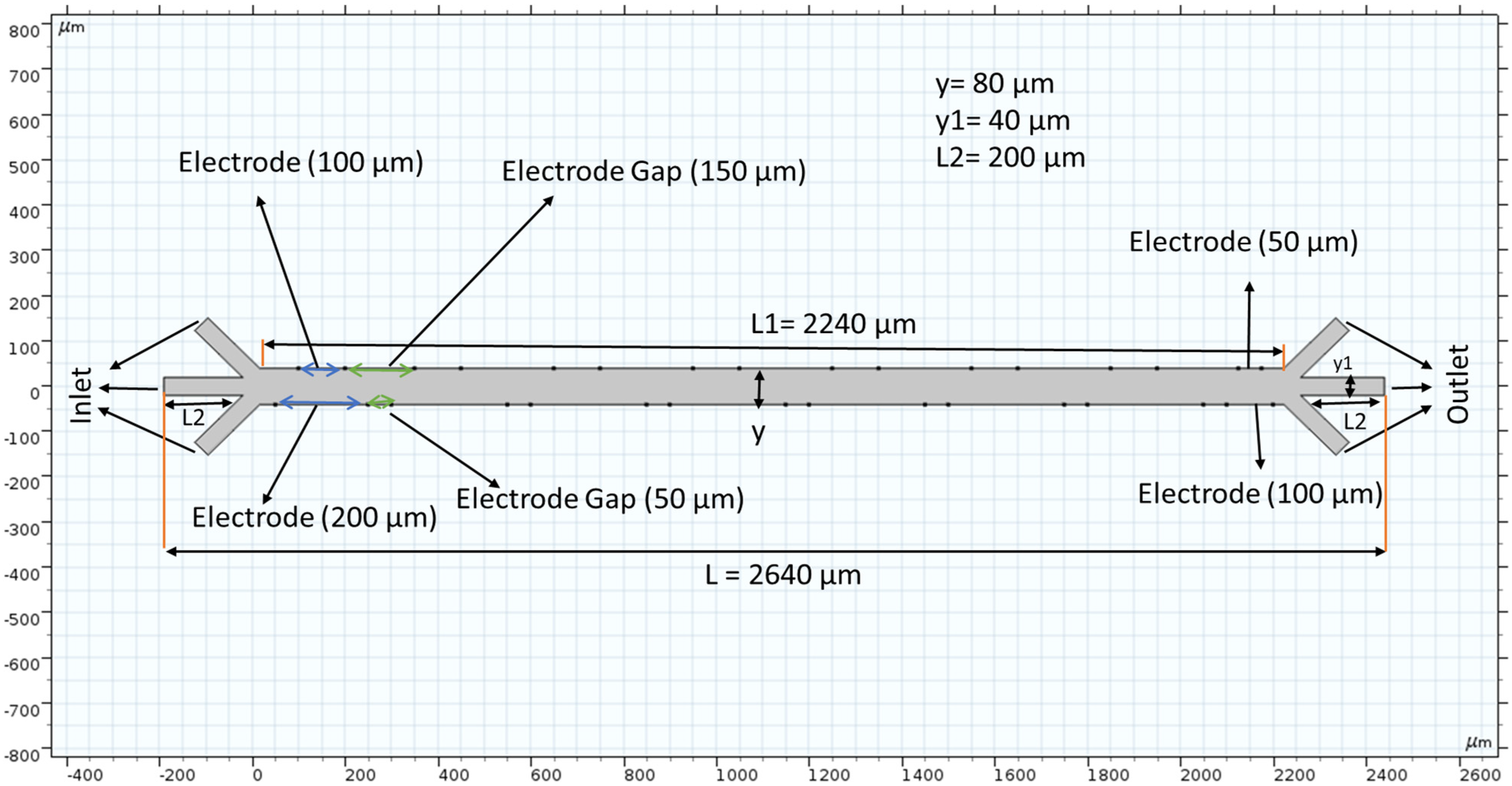
2.2. Schematic
2.3. Boundary Conditions
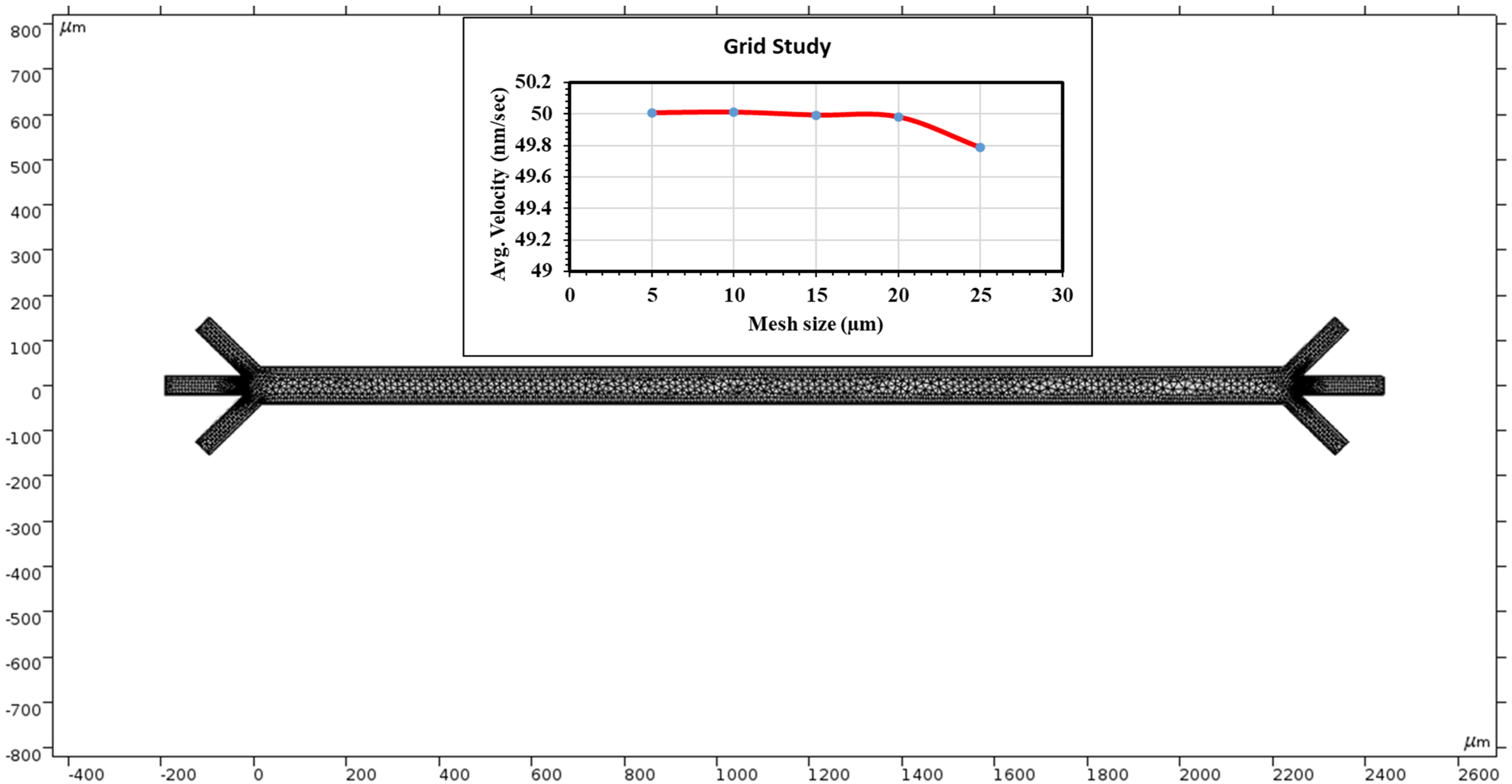
2.4. Mesh
2.5. AI-Use Acknowledgement
3. Simulations and Results
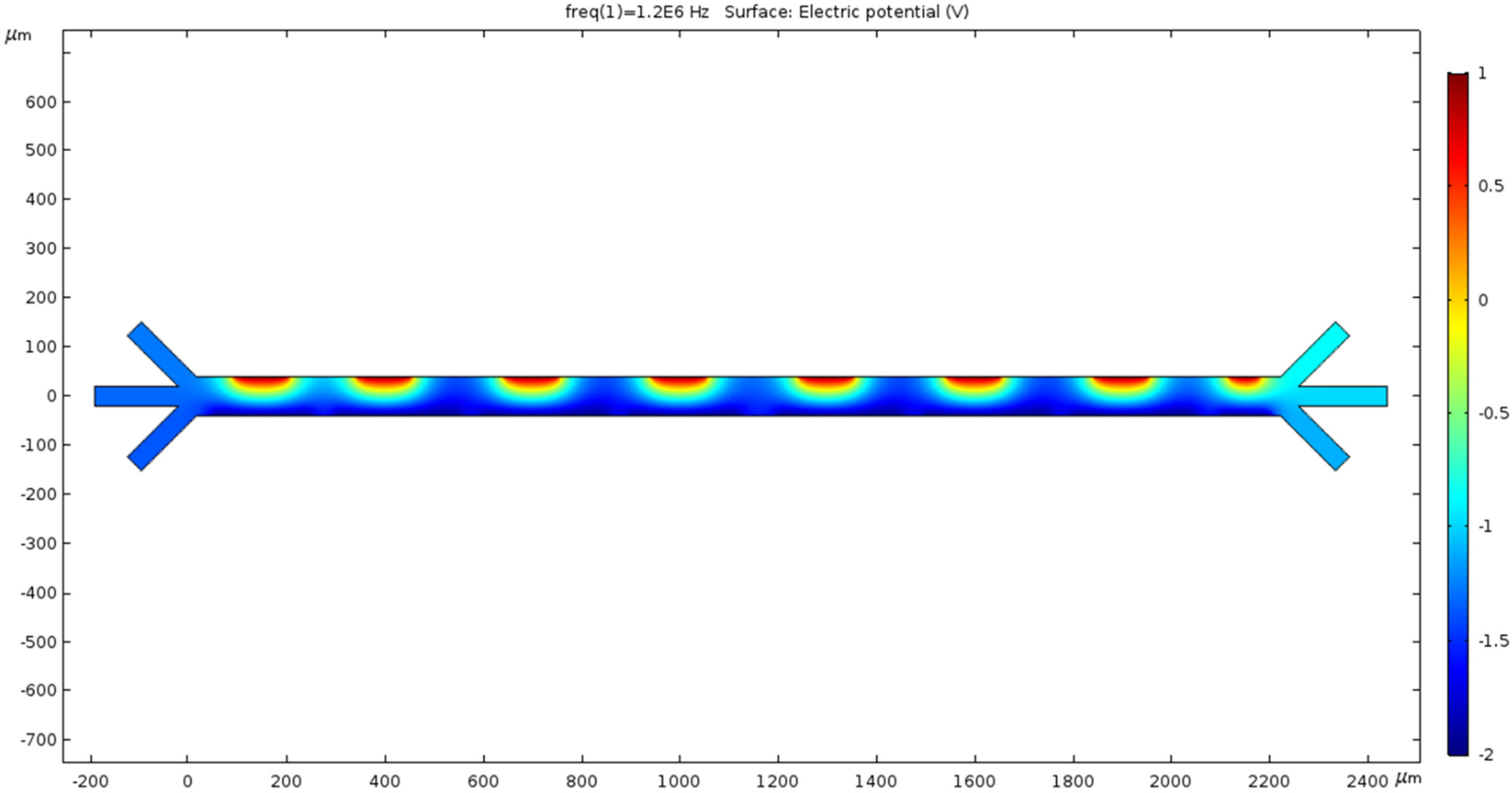
3.1. Voltage Induced in the Microchannel
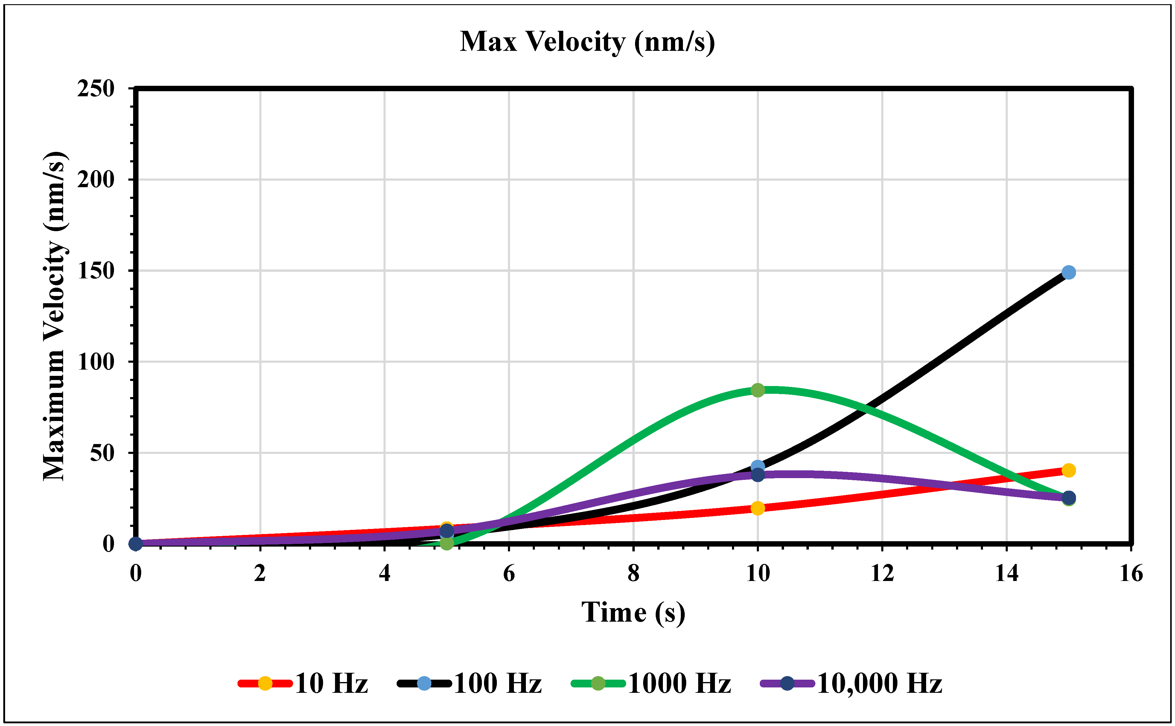
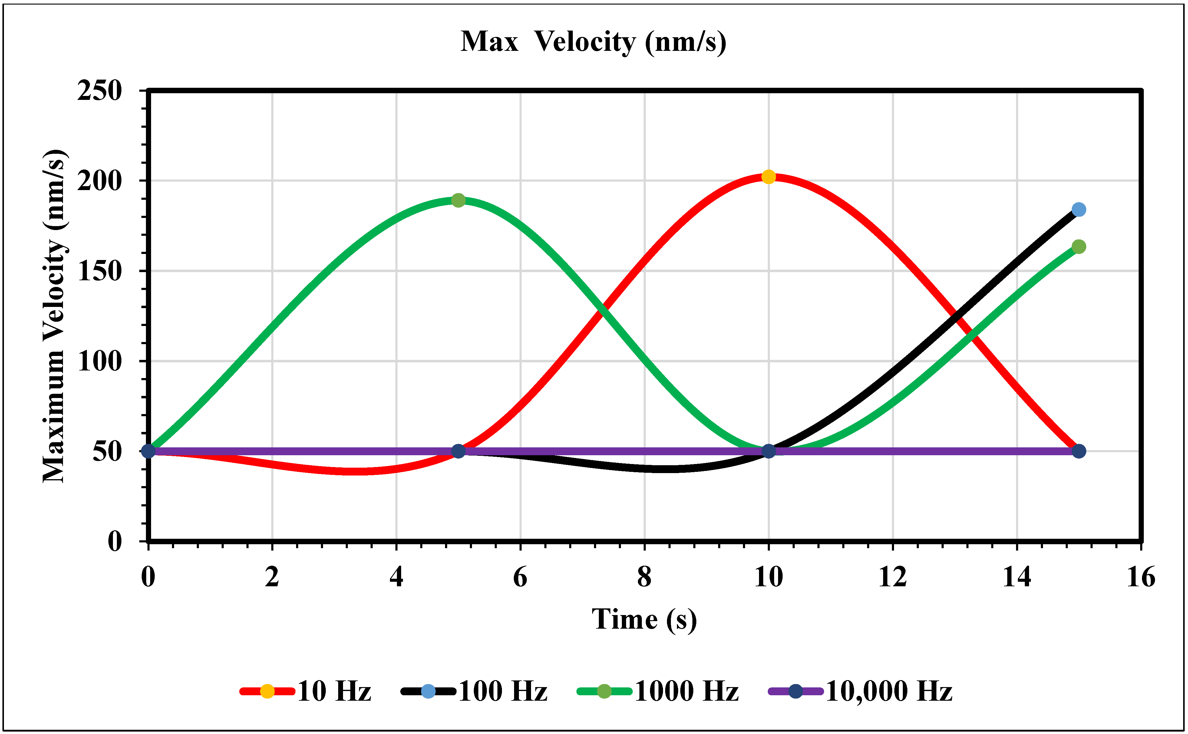
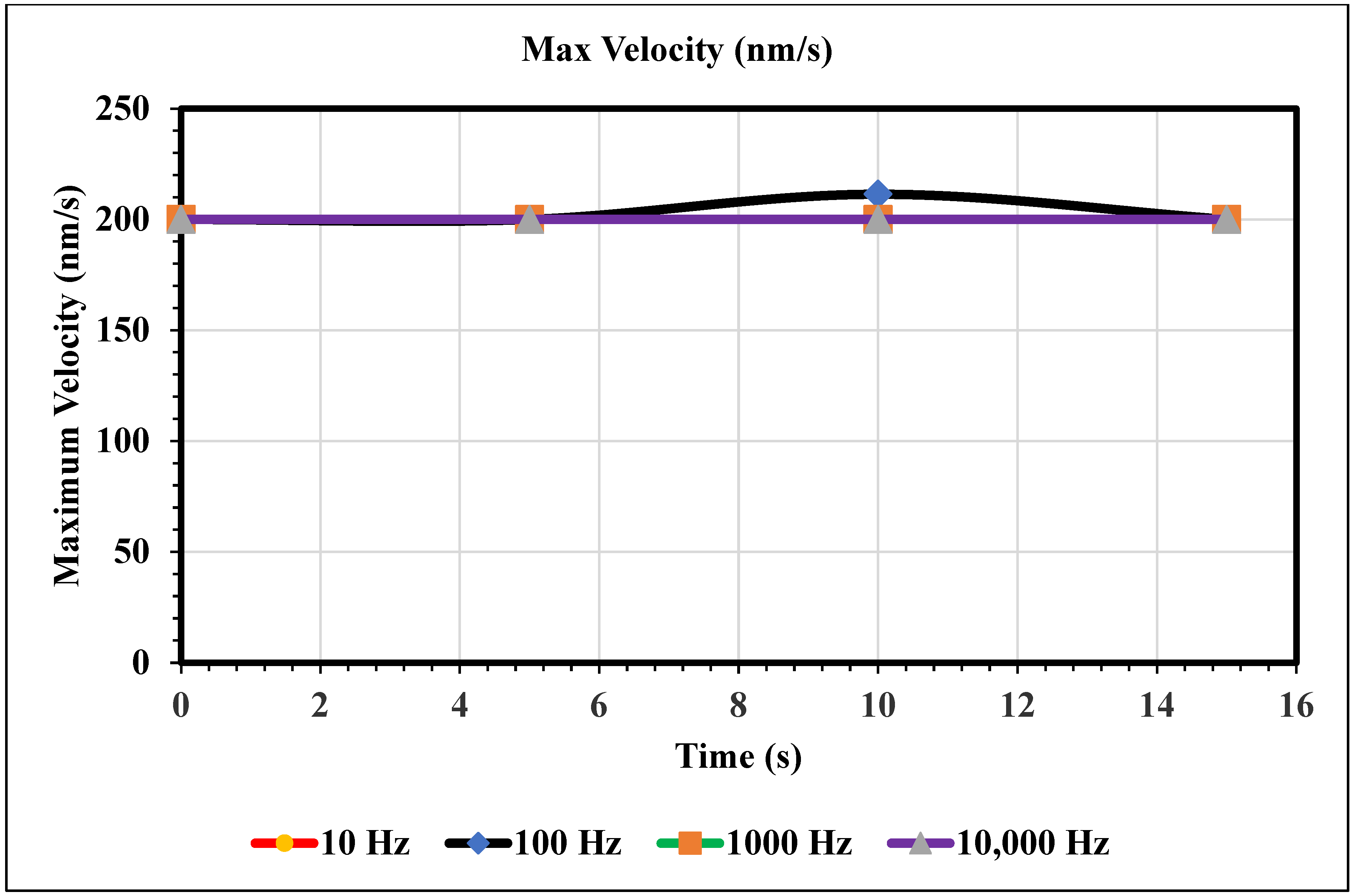
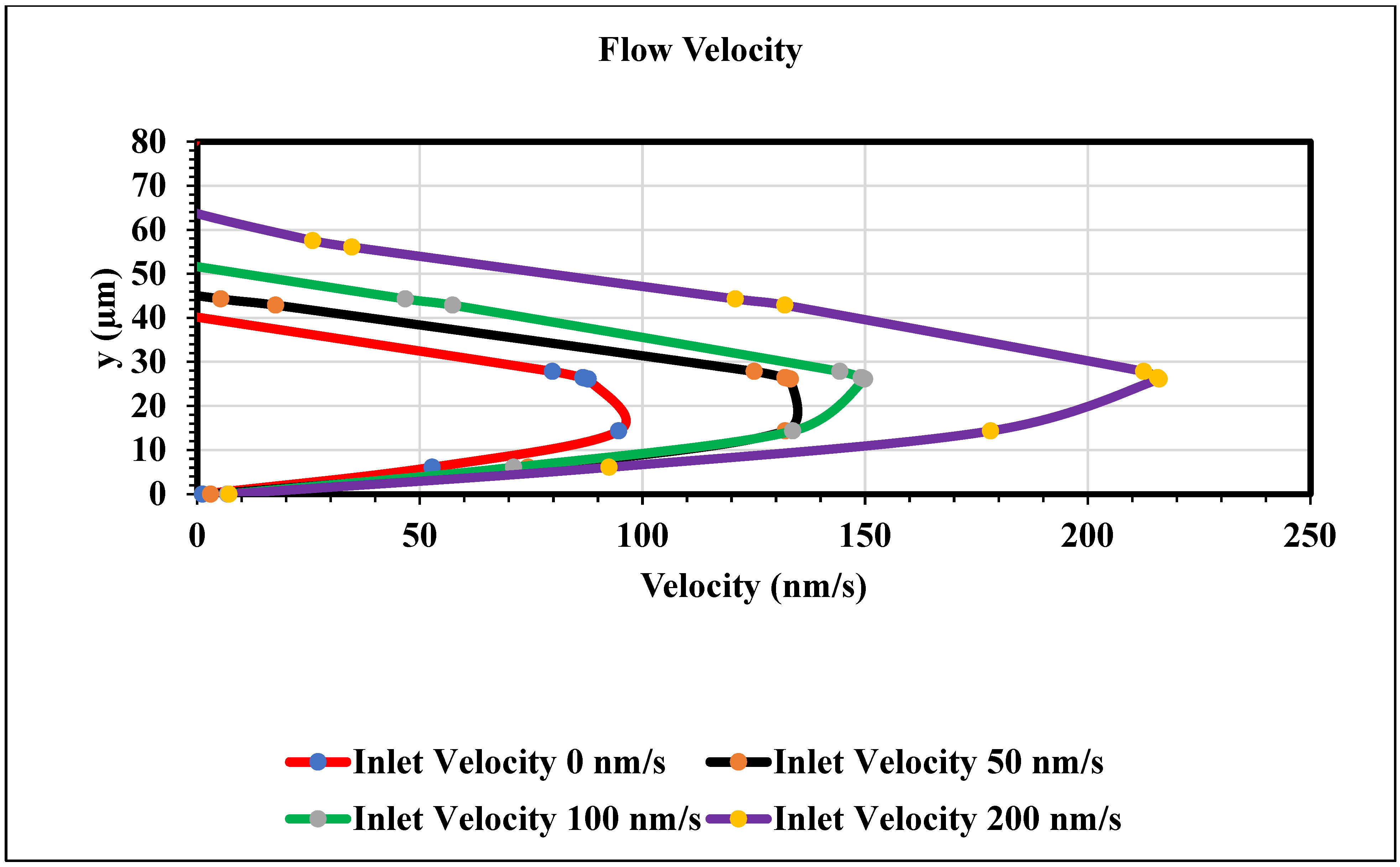
3.2. Microchannel Fluid Velocities Trialed
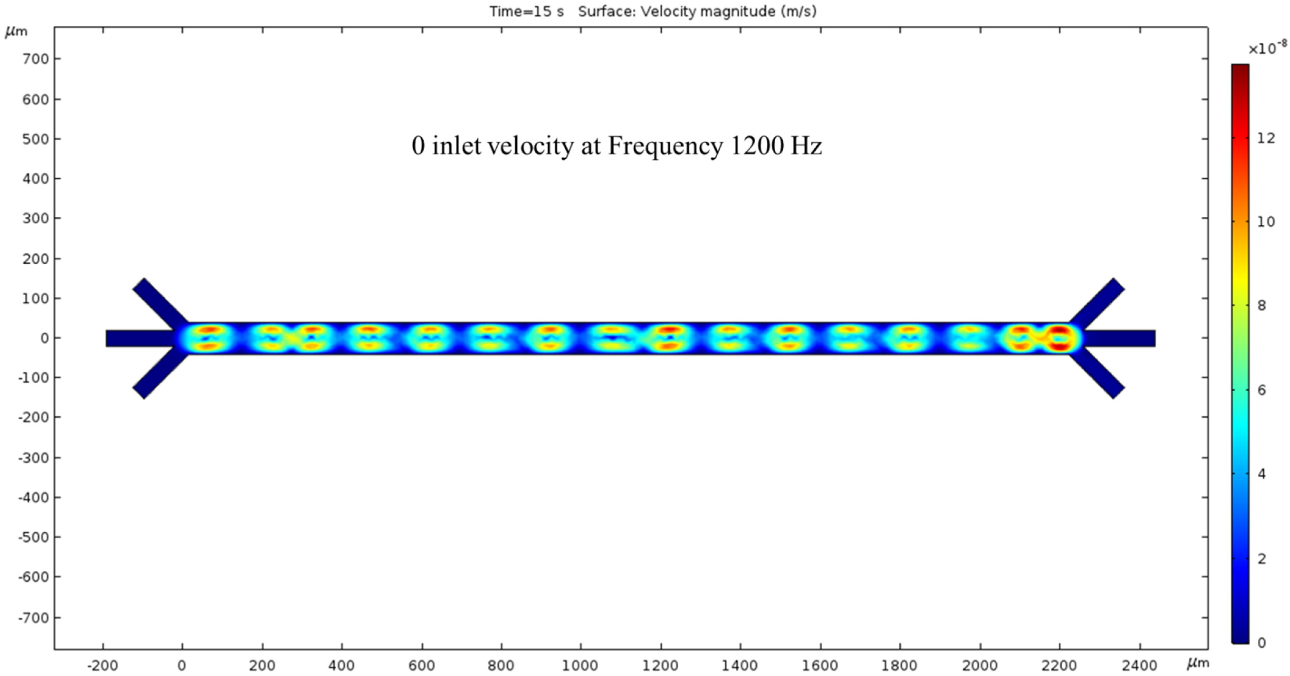
3.2.1. 0 nm/s
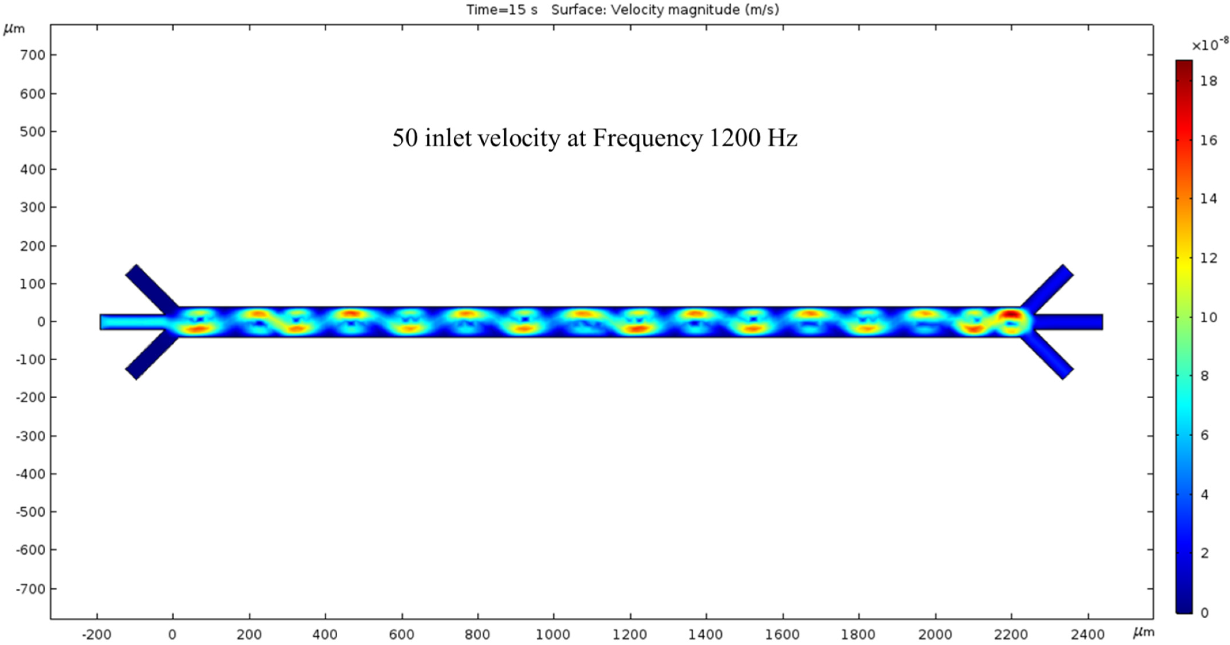
3.2.2. Trial of 50 nm/s Fluid Velocity
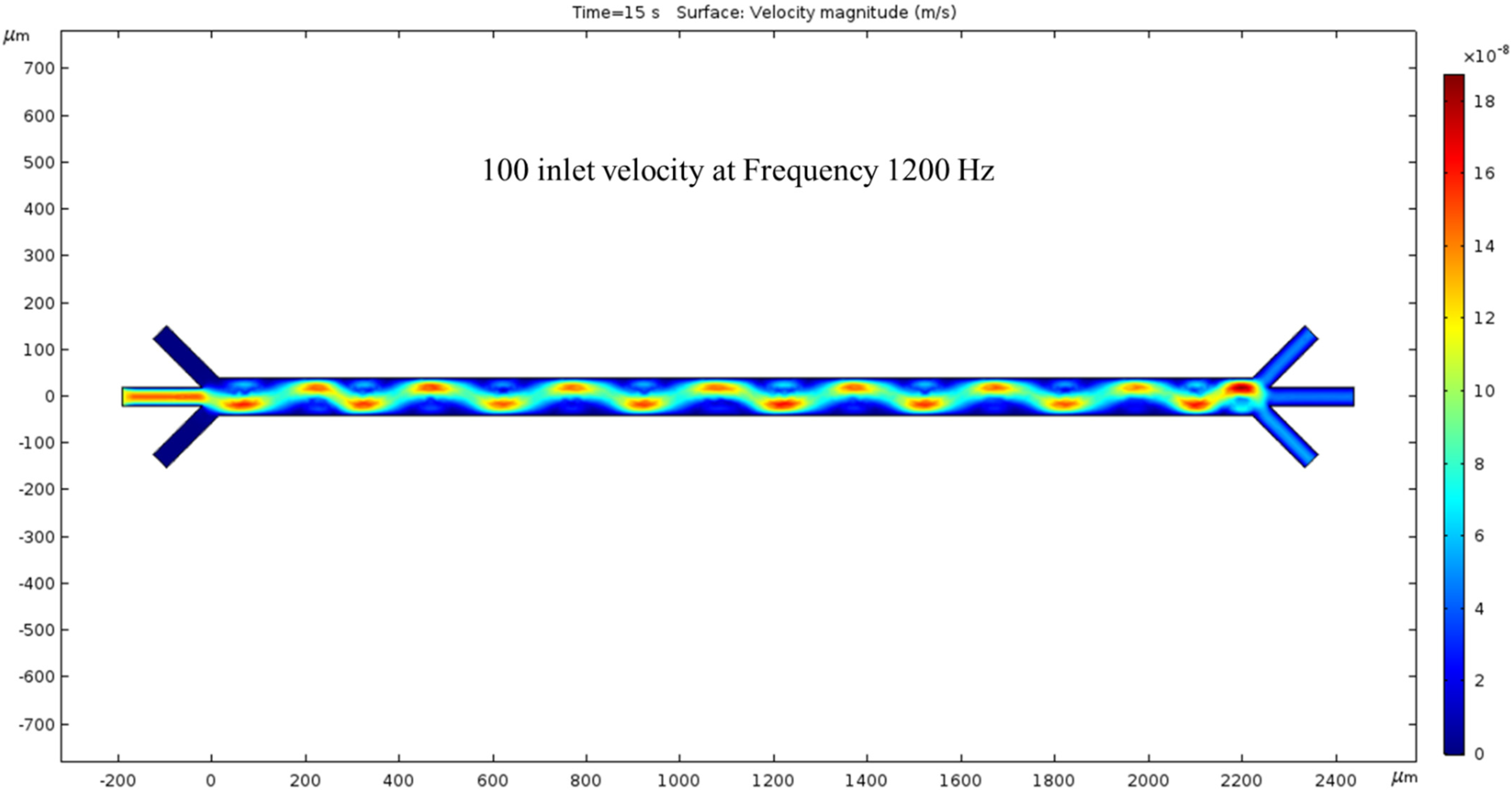
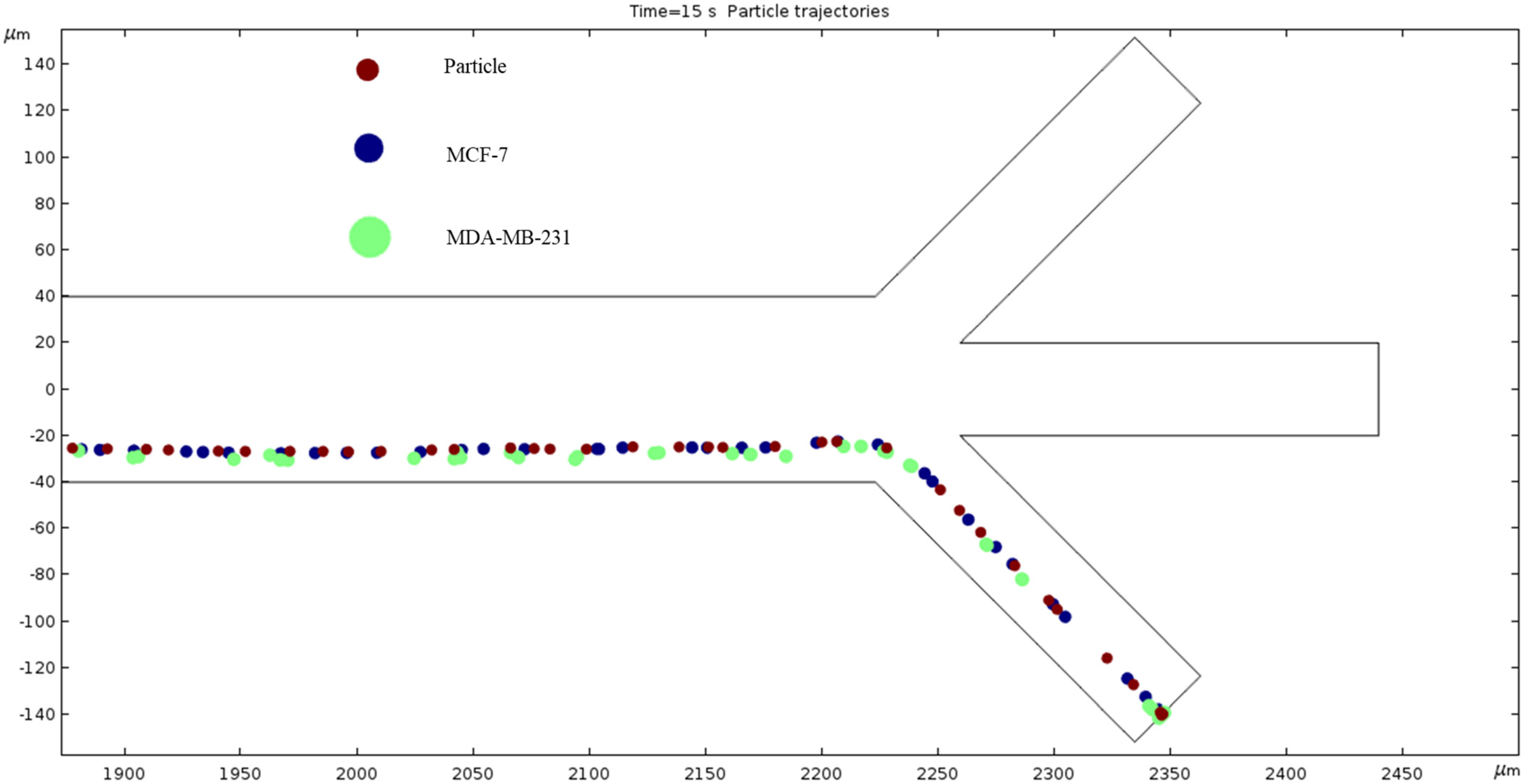
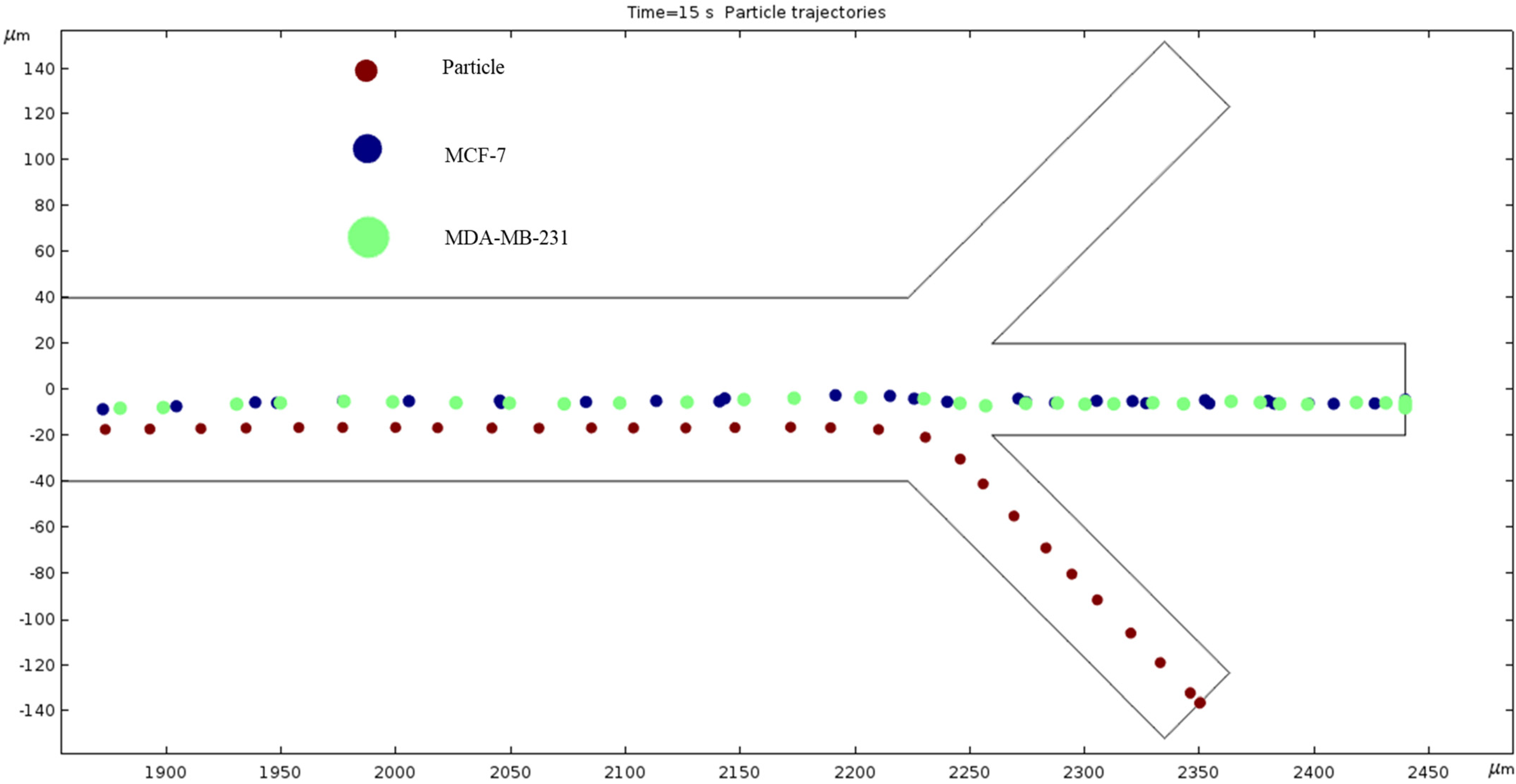
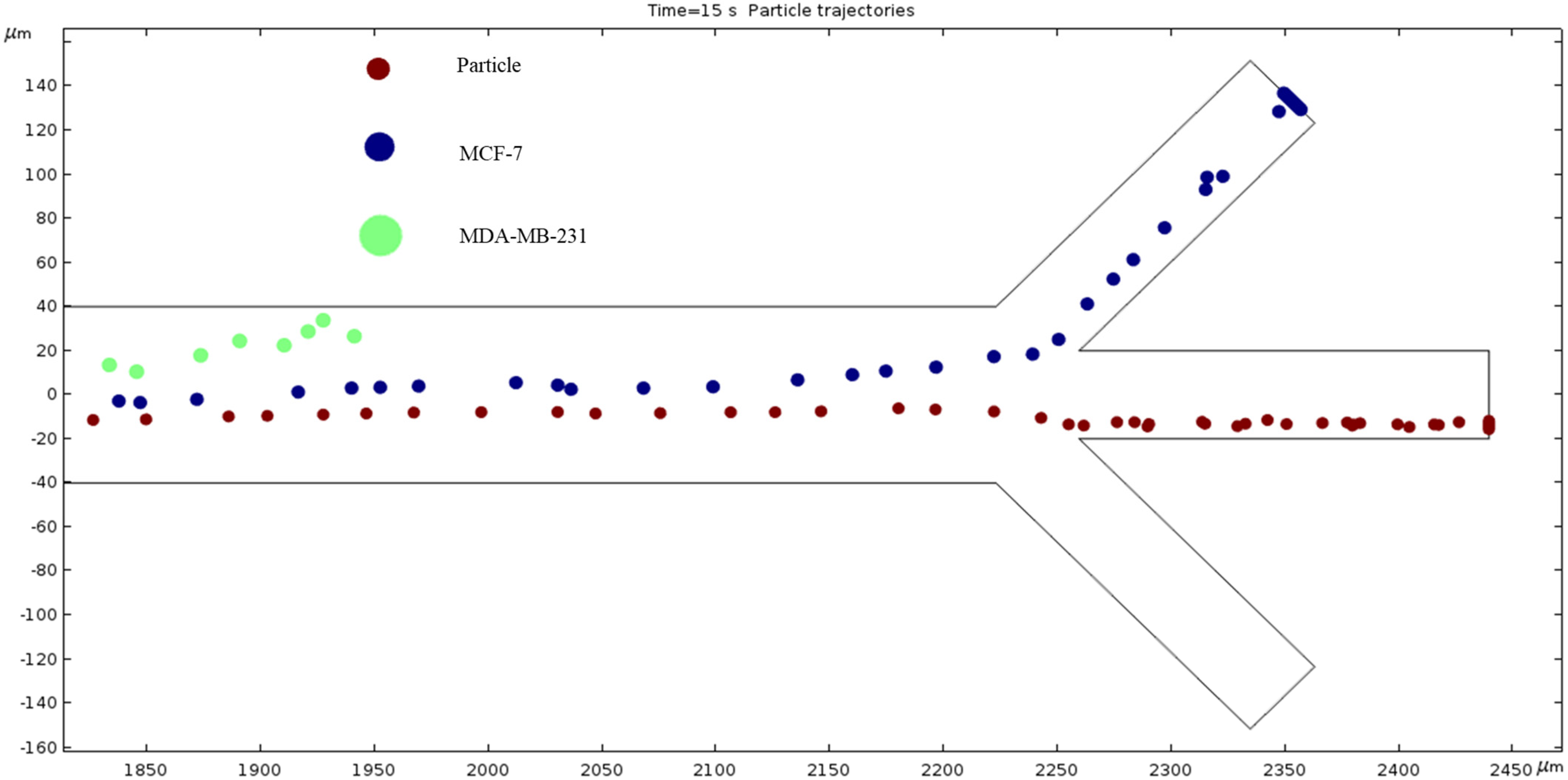
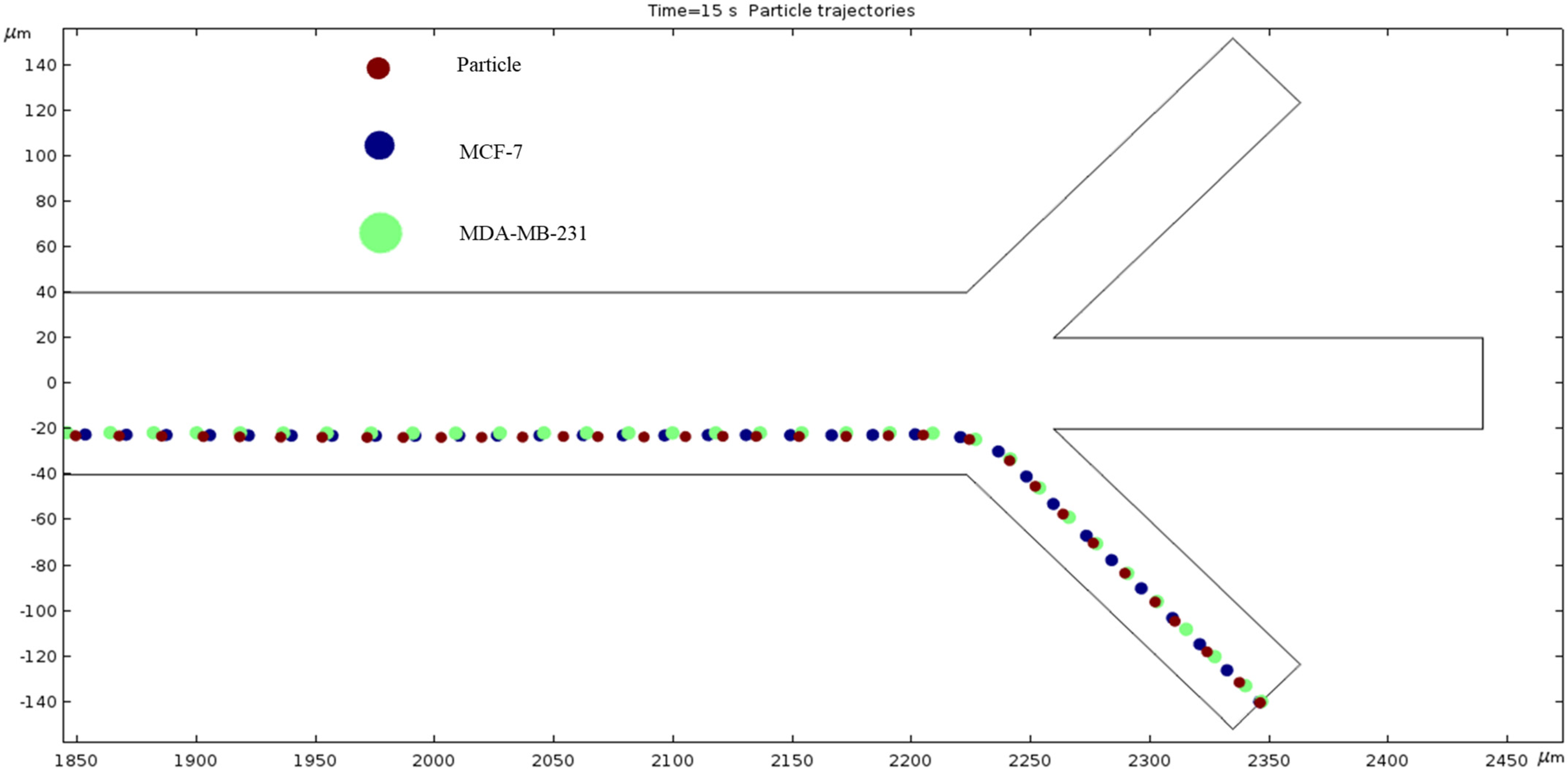
3.2.3. Trial of 100 nm/s Fluid Velocity
4. Discussion
5. Conclusions
Supplementary Materials
Author Contributions
Funding
Data Availability Statement
Acknowledgments
Conflicts of Interest
References
- Karniadakis, G.; Beskok, A.; Aluru, N. Microflows and Nanoflows: Fundamentals and Simulation; Springer Science & Business Media: Berlin/Heidelberg, Germany, 2006; Volume 29. [Google Scholar]
- Hsu, W.-L.; Daiguji, H. Manipulation of Protein Translocation through Nanopores by Flow Field Control and Application to Nanopore Sensors. Anal. Chem. 2016, 88, 9251–9258. [Google Scholar] [CrossRef]
- Chen, X.; Zhang, S.; Zhang, L.; Yao, Z.; Chen, X.; Zheng, Y.; Liu, Y. Applications and theory of electrokinetic enrichment in micro-nanofluidic chips. Biomed. Microdevices 2017, 19, 19. [Google Scholar] [CrossRef] [PubMed]
- Mondal, K.; Ali, M.A.; Srivastava, S.; Malhotra, B.D.; Sharma, A. Electrospun functional micro/nanochannels embedded in porous carbon electrodes for microfluidic biosensing. Sens. Actuators B Chem. 2016, 229, 82–91. [Google Scholar] [CrossRef]
- Matteucci, M.; Heiskanen, A.; Zór, K.; Emnéus, J.; Taboryski, R. Comparison of ultrasonic welding and thermal bonding for the integration of thin film metal electrodes in injection molded polymeric lab-on-chip systems for electrochemistry. Sensors 2016, 16, 1795. [Google Scholar] [CrossRef] [PubMed]
- Hsieh, T.C.; Wijeratne, E.K.; Liang, J.Y.; Gunatilaka, A.L.; Wu, J.M. Differential control of growth, cell cycle progression, and expression of NF-κB in human breast cancer cells MCF-7, MCF-10A, and MDA-MB-231 by ponicidin and oridonin, diterpenoids from the chinese herb Rabdosia rubescens. Biochem. Biophys. Res. Commun. 2005, 337, 224–231. [Google Scholar] [CrossRef] [PubMed]
- Moses, S.L.; Edwards, V.M.; Brantley, E. Cytotoxicity in MCF-7 and MDA-MB-231 breast cancer cells, without harming MCF-10A healthy cells. J. Nanomed. Nanotechnol. 2016, 7, 1–11. [Google Scholar]
- Isfahani, A.M.; Tasdighi, I.; Karimipour, A.; Shirani, E.; Afrand, M. A joint lattice Boltzmann and molecular dynamics investigation for thermohydraulical simulation of nano flows through porous media. Eur. J. Mech.-B/Fluids 2016, 55, 15–23. [Google Scholar] [CrossRef]
- Meghdadi Isfahani, A.H. Parametric study of rarefaction effects on micro-and nanoscale thermal flows in porous structures. J. Heat Transf. 2017, 139, 092601. [Google Scholar] [CrossRef]
- Bagi, M.; Amjad, F.; Ghoreishian, S.M.; Sohrabi Shahsavari, S.; Huh, Y.S.; Moraveji, M.K.; Shimpalee, S. Advances in technical assessment of spiral inertial microfluidic devices toward bioparticle separation and profiling: A critical review. BioChip J. 2024, 18, 1–23. [Google Scholar] [CrossRef]
- Hettiarachchi, S.; Cha, H.; Ouyang, L.; Mudugamuwa, A.; An, H.; Kijanka, G.; Kashaninejad, N.; Nguyen, N.-T.; Zhang, J. Recent microfluidic advances in submicron to nanoparticle manipulation and separation. Lab Chip 2023, 23, 982–1010. [Google Scholar] [CrossRef]
- Dutta, D.; Smith, K.; Palmer, X. Long-Range ACEO Phenomena in Microfluidic Channel. Surfaces 2023, 6, 145–163. [Google Scholar] [CrossRef]
- Suh, Y.K.; Kang, S. A Review on Mixing in Microfluidics. Micromachines 2010, 1, 82–111. [Google Scholar] [CrossRef]
- Chang, C.-C.; Yang, R.-J. Electrokinetic mixing in microfluidic systems. Microfluid. Nanofluid. 2007, 3, 501–525. [Google Scholar] [CrossRef]
- Rashidi, S.; Bafekr, H.; Valipour, M.S.; Esfahani, J.A. A review on the application, simulation, and experiment of the electrokinetic mixers. Chem. Eng. Process. Process. Intensif. 2018, 126, 108–122. [Google Scholar] [CrossRef]
- Johnson, T.J.; Ross, A.D.; Locascio, L.E. Rapid Microfluidic Mixing. Anal. Chem. 2002, 74, 45–51. [Google Scholar] [CrossRef] [PubMed]
- Glasgow, I.; Aubry, N. Enhancement of microfluidic mixing using time pulsing. Lab Chip 2003, 3, 114–120. [Google Scholar] [CrossRef] [PubMed]
- Shang, X.; Huang, X.; Yang, C. Vortex generation and control in a microfluidic chamber with actuations. Phys. Fluids 2016, 28, 122001. [Google Scholar] [CrossRef]
- Daghighi, Y.; Li, D. Numerical study of a novel induced-charge electrokinetic micro-mixer. Anal. Chim. Acta 2013, 763, 28–37. [Google Scholar] [CrossRef] [PubMed]
- Qian, S.; Bau, H.H. Magneto-hydrodynamics based microfluidics. Mech. Res. Commun. 2009, 36, 10–21. [Google Scholar] [CrossRef]
- Cai, G.; Xue, L.; Zhang, H.; Lin, J. A Review on Micromixers. Micromachines 2017, 8, 274. [Google Scholar] [CrossRef]
- Sigdel, I.; Gupta, N.; Faizee, F.; Khare, V.M.; Tiwari, A.K.; Tang, Y. Biomimetic microfluidic platforms for the assessment of breast cancer metastasis. Front. Bioeng. Biotechnol. 2021, 9, 633671. [Google Scholar] [CrossRef] [PubMed]
- Dutta, D.; Palmer, X.L.; Ortega-Rodas, J.; Balraj, V.; Dastider, I.G.; Chandra, S. Biomechanical and Biophysical Properties of Breast Cancer cells under varying glycemic regimens. Breast Cancer Basic Clin. Res. 2020, 14, 1178223420972362. [Google Scholar] [CrossRef] [PubMed]
- Dutta, D.; Russell, C.; Kim, J.; Chandra, S. Differential mobility of breast cancer cells and normal breast epithelial cells under DC electrophoresis and electroosmosis. Anticancer Res. 2018, 38, 5733–5738. [Google Scholar] [CrossRef] [PubMed]
- Jubery, T.Z.; Dutta, P. A fast algorithm to predict cell trajectories in microdevices using dielectrophoresis. Numer. Heat Transf. Part A Appl. 2013, 64, 107–131. [Google Scholar] [CrossRef]
- Shirmohammadli, V.; Manavizadeh, N. Numerical modeling of cell trajectory inside a dielectrophoresis microdevice designed for breast cancer cell screening. IEEE Sens. J. 2018, 18, 8215–8222. [Google Scholar] [CrossRef]
- DM Campos, C.; Uning, K.T.; Barmuta, P.; Markovic, T.; Yadav, R.; Mangraviti, G.; Ocket, I.; Van Roy, W.; Lagae, L.; Liu, C. Use of high frequency electrorotation to identify cytoplasmic changes in cells non-disruptively. Biomed. Microdevices 2023, 25, 39. [Google Scholar] [CrossRef] [PubMed]
- Doh, I.; Cho, Y.H. A continuous cell separation chip using hydrodynamic dielectrophoresis (DEP) process. Sens. Actuators A Phys. 2005, 121, 59–65. [Google Scholar] [CrossRef]
- Farasat, M.; Aalaei, E.; Kheirati Ronizi, S.; Bakhshi, A.; Mirhosseini, S.; Zhang, J.; Nguyen, N.-T.; Kashaninejad, N. Signal-Based Methods in Dielectrophoresis for Cell and Particle Separation. Biosensors 2022, 12, 510. [Google Scholar] [CrossRef]
- Huang, Y.; Holzel, R.; Pethig, R.; Wang, X.B. Differences in the AC electrodynamics of viable and non-viable yeast cells determined through combined dielectrophoresis and electrorotation studies. Phys. Med. Biol. 1992, 37, 1499. [Google Scholar] [CrossRef] [PubMed]
- Mei, L.; Cui, D.; Shen, J.; Dutta, D.; Brown, W.; Zhang, L.; Dabipi, I.K. Electroosmotic mixing of non-newtonian fluid in a microchannel with obstacles and zeta potential heterogeneity. Micromachines 2021, 12, 431. [Google Scholar] [CrossRef]
- TruongVo, T.N.; Kennedy, R.M.; Chen, H.; Chen, A.; Berndt, A.; Agarwal, M.; Zhu, L.; Nakshatri, H.; Wallace, J.; Na, S.; et al. Microfluidic channel for characterizing normal and breast cancer cells. J. Micromech. Microeng. 2017, 27, 035017. [Google Scholar] [CrossRef]


| Cell Name | Diameter (µm) | Conductivity (S/m) | Relative Permittivity |
|---|---|---|---|
| Particles | 10 | 2.00 × 10⁻¹ | 40 |
| MCF-7 | 11.2 | 2.50 × 10⁻¹ | 50 |
| MDA-MB-231 | 12.4 | 3.10 × 10⁻¹ | 59 |
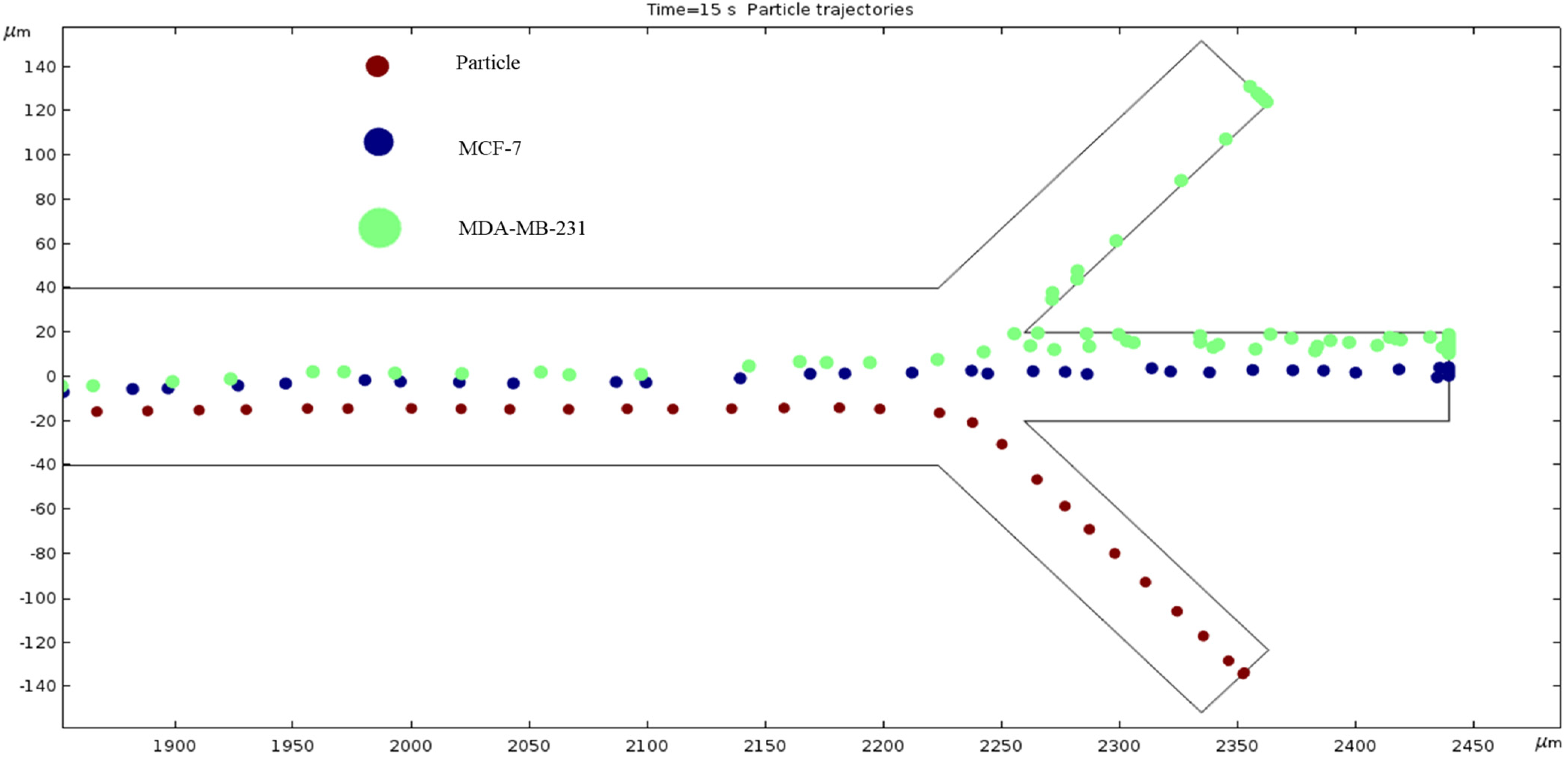
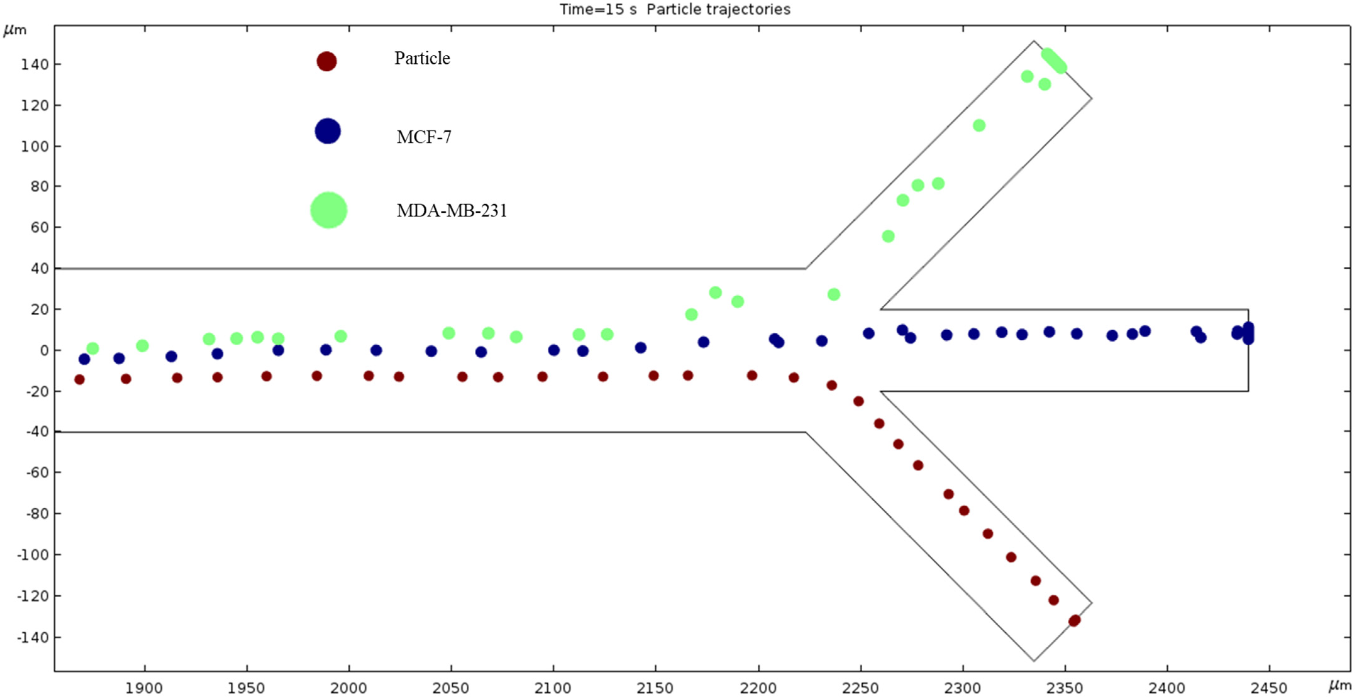
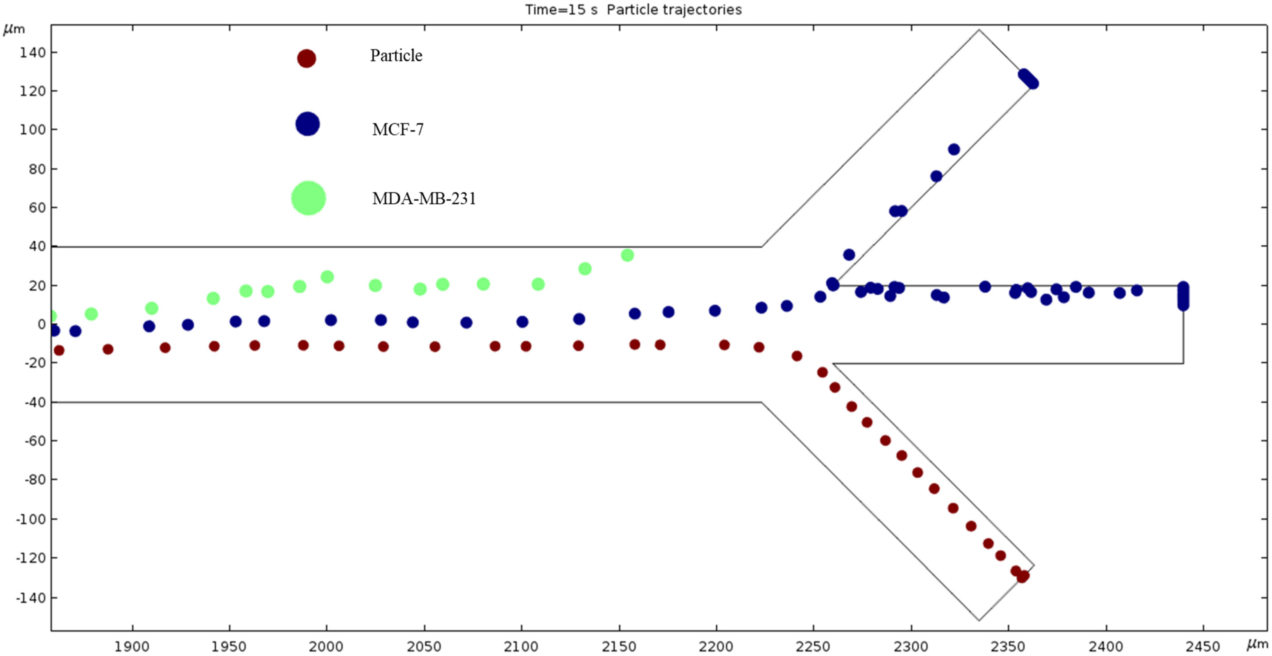
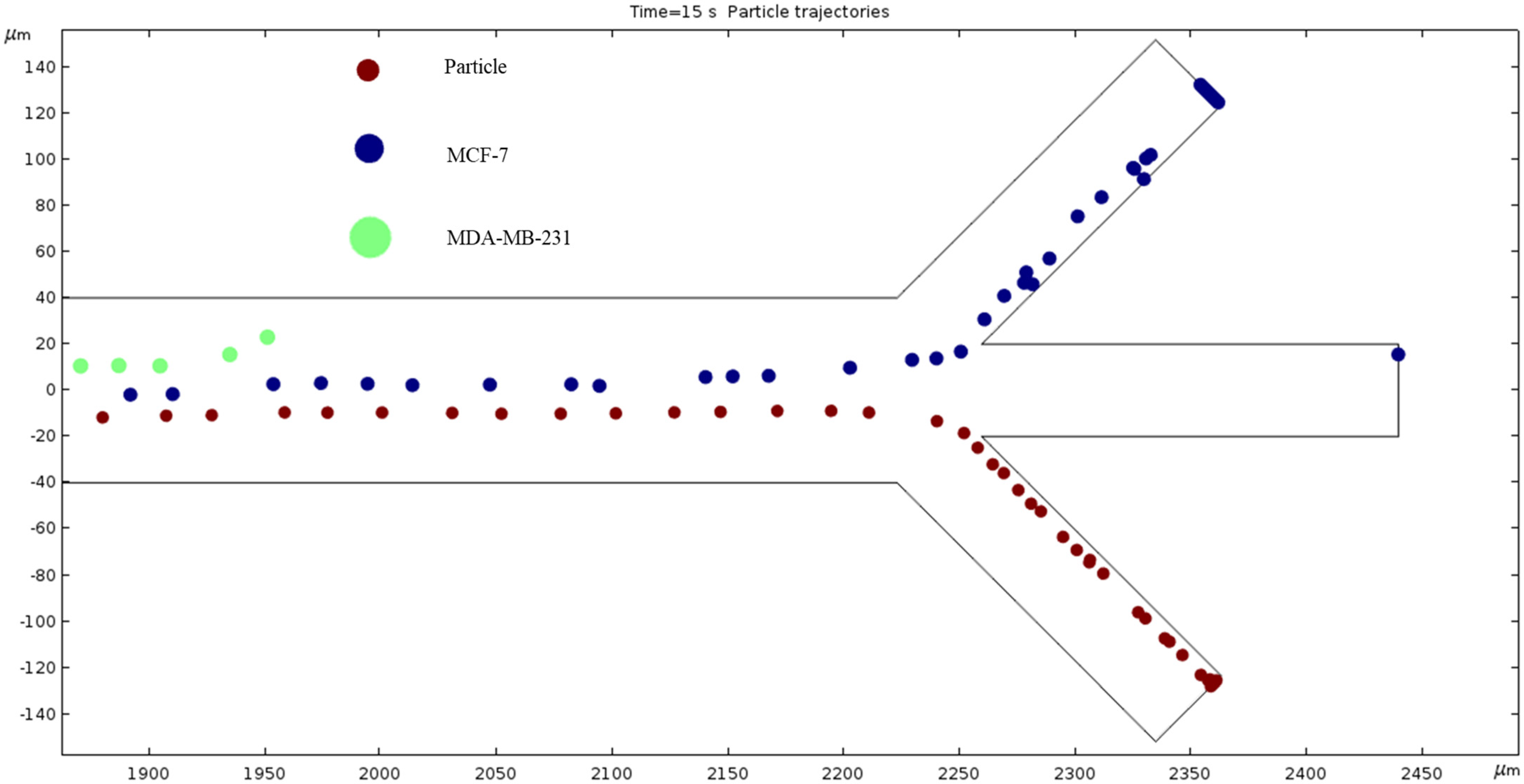
| Frequency | Separation in Outlet | ||
|---|---|---|---|
| Bottom | Middle | Top | |
| 10 KHz | Particles, MCF7, MDA-MB-231 | ||
| 100 KHz | Particles, MCF7, MDA-MB-231 | ||
| 800 KHz | Particles | MCF7, MDA-MB-231 | |
| 1000 KHz | Particles | MCF7, MDA-MB-231 | MDA-MB-231 |
| 1200 KHz | Particles | MCF7 | MDA-MB-231 |
| 1500 KHz | Particles | MCF7 | MCF7 |
| 2000 KHz | Particles | MCF7 | |
| 3000 KHz | Particles | MCF7 | |
| 5000 KHz | Particles | MCF7 | |
| 10,000 KHz | Particles | MCF7 | |
| 100,000 KHz | Particles, MCF7, MDA-MB-231 | ||
Disclaimer/Publisher’s Note: The statements, opinions and data contained in all publications are solely those of the individual author(s) and contributor(s) and not of MDPI and/or the editor(s). MDPI and/or the editor(s) disclaim responsibility for any injury to people or property resulting from any ideas, methods, instructions or products referred to in the content. |
© 2024 by the authors. Licensee MDPI, Basel, Switzerland. This article is an open access article distributed under the terms and conditions of the Creative Commons Attribution (CC BY) license (https://creativecommons.org/licenses/by/4.0/).
Share and Cite
Dutta, D.; Palmer, X.; Lim, J.Y.; Chandra, S. Simulation on the Separation of Breast Cancer Cells within a Dual-Patterned End Microfluidic Device. Fluids 2024, 9, 123. https://doi.org/10.3390/fluids9060123
Dutta D, Palmer X, Lim JY, Chandra S. Simulation on the Separation of Breast Cancer Cells within a Dual-Patterned End Microfluidic Device. Fluids. 2024; 9(6):123. https://doi.org/10.3390/fluids9060123
Chicago/Turabian StyleDutta, Diganta, Xavier Palmer, Jung Yul Lim, and Surabhi Chandra. 2024. "Simulation on the Separation of Breast Cancer Cells within a Dual-Patterned End Microfluidic Device" Fluids 9, no. 6: 123. https://doi.org/10.3390/fluids9060123
APA StyleDutta, D., Palmer, X., Lim, J. Y., & Chandra, S. (2024). Simulation on the Separation of Breast Cancer Cells within a Dual-Patterned End Microfluidic Device. Fluids, 9(6), 123. https://doi.org/10.3390/fluids9060123