Unsteady Multiphase Simulation of Oleo-Pneumatic Shock Absorber Flow

Abstract

The internal flow in oleo-pneumatic shock absorbers is a complex multiphysics problem combining the interaction between highly unsteady turbulent flow and multiphase mixing, among other effects. The aim is to present a validated simulation methodology that facilitates shock absorber performance prediction by capturing the dominant internal flow physics. This is achieved by simulating a drop test of approximately 1 tonne with an initial contact vertical speed of 2.7 m/s, corresponding to a light jet. The flow field solver is ANSYS Fluent, using an unsteady two-dimensional axisymmetric multiphase setup with a time-varying inlet velocity boundary condition corresponding to the stroke rate of the shock absorber piston. The stroke rate is calculated using a two-equation dynamic system model of the shock absorber under the applied loading. The simulation is validated against experimental measurements of the total force on the shock absorber during the stroke, in addition to standard physical checks. The flow field analysis focuses on multiphase mixing and its influence on the turbulent free shear layer and recirculating flow. A mixing index approach is suggested to facilitate systematically quantifying the mixing process and identifying the distinct stages of the interaction. It is found that gas–oil interaction has a significant impact on the flow development in the shock absorber’s upper chamber, where strong mixing leads to a periodic stream of small gas bubbles being fed into the jet’s shear layer from larger bubbles in recirculation zones, most notably in the corner between the orifice plate and outer shock absorber wall.

1. Introduction

1.1. Background

Oleo-pneumatic shock absorbers (OPSAs) have been the standard choice in aircraft landing gear designs for decades, largely due to their high efficiency (energy dissipation per unit weight) [1,2]. Yet, despite the huge leaps in computational methods and power over the years, the internal dynamics of OPSAs remain a challenging problem to simulate, owing to the multiphysics nature of the flow, the complex geometry, and the scarcity of validation data in the public literature. These difficulties manifest in the scarcity of data on OPSA internal flows, leading to a large gap in the present literature around practical methods of simulating OPSAs and predicting their performance.

The main mechanism of energy dissipation in OPSAs usually consists of hydraulic resistance to the flow through an orifice or contraction, leading to strongly turbulent free shear flow in the downstream region (in the upper chamber) [2,3,4]. The hydraulic resistance level can vary during the stroke and can be strongly impacted by different forms of multiphase interaction that could occur, depending on the specific internal design of the shock absorber and the external disturbance applied to the system. General mixing, aeration, foaming, and cavitation, among other phenomena, can modify the effective properties of the working fluid and impact performance [4]. Therefore, as well as understanding the flow conditions in the vicinity of the orifice [5], it is also important to consider the multiphase mixing taking place inside the shock absorber, and its potential impact on performance. However, in order to predict performance reliably, extensive validation must be conducted. The present work is a first step in which an OPSA simulation of a drop test is validated against experimental measurements, and its internal field is discussed.

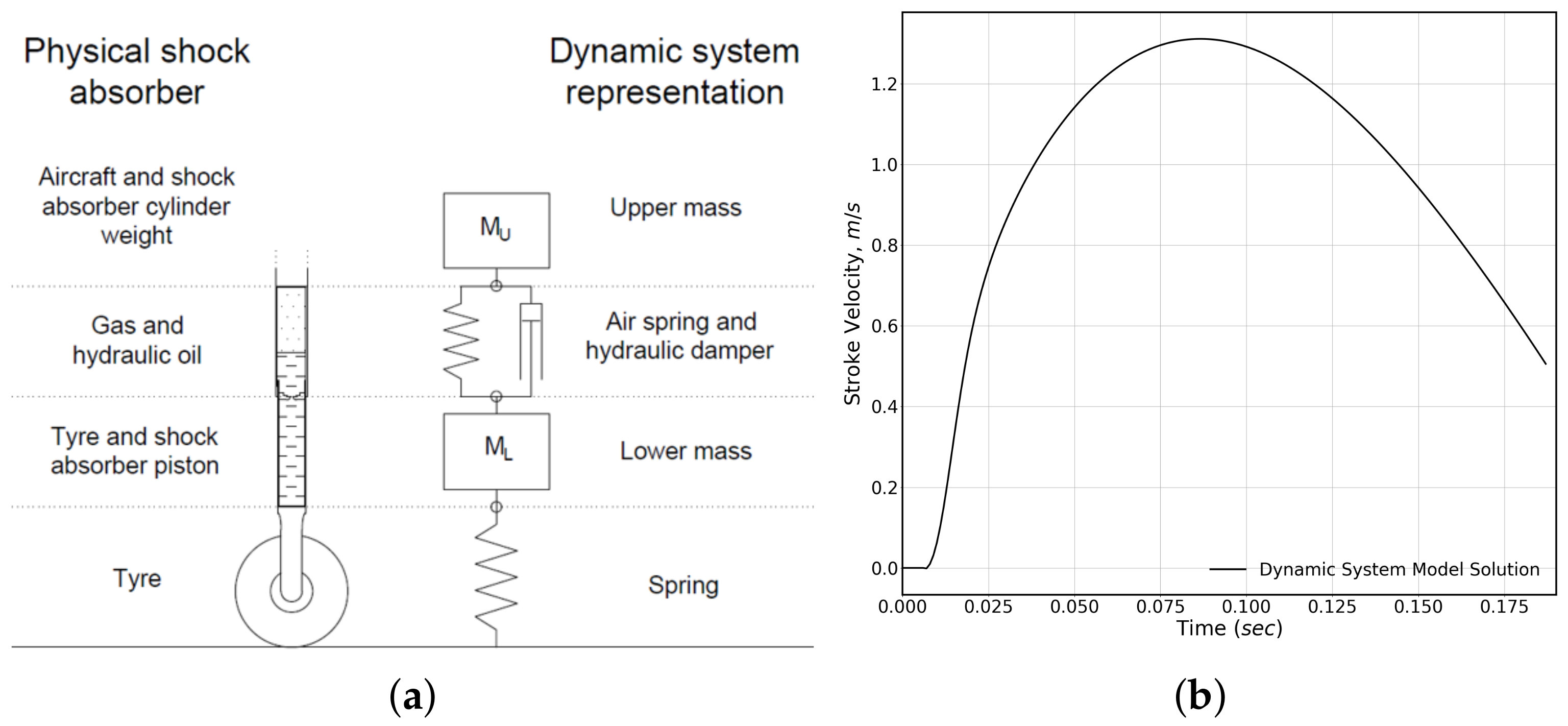
1.2. Oleo-Pneumatic Shock Absorber Modelling

Most of the earlier shock absorber modelling effort concentrated on the development of system-level dynamic models, using mass–spring–damper models and force balance equations of varying complexity, representing the shock absorber system under investigation. This includes the modelling of a small military trainer jet OPSA by Miltwitzky and Cook [3] and the modelling of the A6-Intruder OPSA conducted by Daniels [6] and Horta et al. [7]. Given the lack of data about the internal processes during an OPSA stroke, these models usually include simplifying assumptions about the properties of the working fluid(s) in the OPSA and key parameters, such as the orifice discharge coefficient. Some work has been conducted on expanding the range of applicability of these methods to involve some multiphysics effects, for example, using more advanced equations of state for the gas phase in OPSAs [8]. Nevertheless, these “low-fidelity” system-level methods are attractive in design studies, e.g., metering pin optimisation [9], and when analysing performance over a wide range of conditions, although they do not provide a basic understanding of the complex internal flow physics that can limit performance in challenging cases.

On the other hand, studies focusing on simulating the internal flow of shock absorbers are less frequent, although they are becoming more popular. Owing to the scarcity of comprehensive experimental studies with the internal geometry and measurement data published, it is rare to find complete validated simulations of an OPSA system using realistic geometry and applying realistic boundary conditions corresponding to a drop test or a realistic landing profile. Studies that have looked at internal flow tend to focus on a main feature of interest, such as the discharge coefficient calculation [10], the turbulent free shear layer development in the orifice nearfield [5], or the impact of orifice diameter and thickness [11]. Different assumptions are used to facilitate these simulations, such as assuming single-phase flow and placing an artificial outflow boundary away from the region of interest [5,10], or using a constant compressing velocity value [11]. Hence, the interaction between the turbulent free shear layer and multiphase flow developing in the upper chamber, under a realistic stroke profile, remains unexplored. This is a gap that the present work aims to at least partially address.

1.3. Multiphase Mixing

The existing literature involving multiphase mixing simulation usually focuses on processes in a specific industrial setting, for example, boiling [12,13,14], which is often considered in the context of refrigeration cycles, or bubble dynamics [15,16,17], which is of particular interest in reactor flows [15,18]. However, heat transfer and buoyancy play a dominant role in the flow development of these studies, which is in contrast to the OPSA flow, where a jet through an orifice plate into a confined chamber usually drives the multiphase interaction. On the other hand, the dam-break problem [19,20,21] provides a valuable insight into some unsteady dynamics and modelling challenges that are relevant to OPSA flows. The validation of computational results against experimental measurements of water waves impacting solid obstacles [22,23,24] underlines the challenges associated with correctly capturing the two-phase unsteady vortex generated by the overturning main water wave and the secondary circulation regions. The OPSA flow is further complicated by being confined within a smaller geometry and by the strong jet and its associated shear layers flowing through the domain.

Furthermore, modelling challenges remain, even in accounting for some basic multiphase dynamics inside OPSAs, such as the interaction between bubbles and their coalescence [15,25,26] or their interaction with solid surfaces [15]. Phenomena that involve a phase change introduce an added layer of complexity due to their potential impact on simulation efficiency and stability, apart from the need for additional validation.

1.4. Turbulence Modelling

Free shear layers are a standard turbulent flow that have been successfully modelled using Reynolds-averaged Navier–Stokes (RANS) closure models in a range of complex configurations, such as open jet wind tunnels [27,28], where these were validated against scale-resolved large eddy simulation results [29], demonstrating that the RANS model can predict the deflection of open jet mixing layers under the influence of an airfoil installed in the potential core. RANS models are often suitable when the free shear layer is initiated by geometry-defined separation, as in the case of most OPSA orifice designs, rather than the effect of an adverse pressure gradient. This makes the use of unsteady RANS-based methods an attractive compromise that accounts for the turbulent shear layer development and main recirculation zones while not being excessively demanding in terms of spatial and temporal resolution. Moreover, RANS models have been found to successfully model turbulence in two-phase bubble columns [25].

An important consideration when applying unsteady RANS methods is the presence of a spectral gap between the frequency of mean flow parameter variation and the frequencies of the modelled turbulent fluctuations [30,31,32]. Such a separation between frequencies is expected in the present case, as the overall stroke frequency is much lower than that of turbulent flow.

1.5. Scope of Present Work

The aim of the present work is to investigate the internal dynamics of an OPSA, particularly focusing on the multiphase interaction. The drop test of Milwitzky and Cook [3] is used as the reference case due to the availability of validation data and sufficient information about the internal geometry. The main novelty of this work is the simulation and analysis of multiphase interaction in a realistic shock absorber geometry under a drop test loading profile, leading to a contribution towards better understanding shock absorber internal dynamics and the quantification of the multiphase mixing process. The impact of this work is expected to promote and enable a more accurate assessment of multiphase effects in the design and performance analysis of shock absorbers, for example, as part of a wider multi-fidelity approach [33].

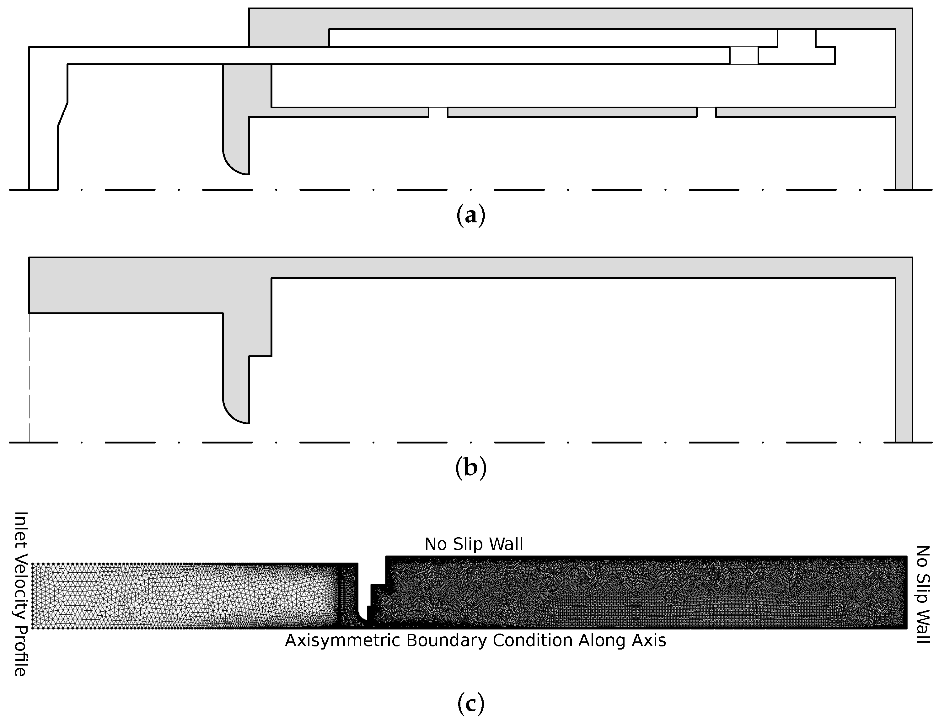
2. Methodology and Computational Setup

The shock absorber used in the drop test [3] is relatively simple, primarily consisting of a fixed orifice plate to provide hydraulic resistance without a metering pin or valve system. Such a simple solution is usually the designer’s first choice, provided that it enables adequate performance and avoids full extension or contraction of the shock absorber under the full range of operational conditions [1]. Nevertheless, the model used in simulations is further simplified to focus on the main multiphase interaction of interest while reducing the geometrical complexity of orifice support tubes, cylinder telescoping bearings, and snubber chamber details, see Figure 1 and Figure 2a,b, particularly since the details of these features are not provided in the available documentation. The computational results are validated against the experimental measurements of Milwitzky and Cook [3], which will be further discussed in the results section.

There are two main options to model the flow inside the shock absorber as it becomes compressed by the telescoping lower wall motion due to an impact. The first is to use a moving mesh algorithm, which allows the physical extent of the computational domain to change with time in accordance with the stroke rate of the shock absorber for a given disturbance. However, this method can lead to degraded mesh quality in critical areas of the computational domain and could add significant computational expense to the overall case. On the other hand, it is possible to simulate the shock absorber stroke using a static mesh with a variable inlet velocity profile that applies the required loading to the shock absorber. This has the advantage of allowing better control over grid quality and being more robust when different loading profiles are used, although it does add some mass into the system (hydraulic oil) to achieve the required loading profile. The second approach is adopted in the present study.

Another challenging aspect of shock absorber multiphase simulations is that the location and shape of the gas–oil interface changes significantly during the simulation; hence, either an adaptive meshing technique or a very fine grid must be used to allow the flow development to be captured accurately. Both of these options add to the cost of simulations. Hence, it is decided, as a compromise, to use a relatively fine upper chamber grid, see Figure 2c, and a 2D axisymmetric boundary condition rather than a full 3D simulation.

A grid convergence study is conducted to establish grid density requirements. Four grid densities are tested, with the most coarse comprising approximately $2\times {10}^4$ cells, while the finest has approximately $4\times {10}^5$ cells. All grids are designed with a higher node density in the upper chamber, downstream of the orifice, to account for the turbulent flow and multiphase mixing taking place there. The results are summarised in

Table 1. Solution grid independence study summary.

Grid	No. of Cells	${\mathit{L}}_{\mathit{SL}}^{\mathit{min}}$$\mathbf{\left(}\mathit{m}\mathbf{\right)}$	${\mathit{L}}_{\mathit{UC}}^{\mathit{max}}$$\mathbf{\left(}\mathit{m}\mathbf{\right)}$	${\mathit{errU}}_{\mathit{CL}}^{\mathit{max}}$	${\mathit{errTi}}_{\mathit{OT}}^{\mathit{max}}$
C1	$1.96\times {10}^4$	$4\times {10}^{-5}$	$6\times {10}^{-3}$	$5.37$%	$2.30$%
C2	$4.88\times {10}^4$	$2\times {10}^{-5}$	$3.7\times {10}^{-3}$	$1.01$%	$0.18$%
C3	$1.34\times {10}^5$	$1\times {10}^{-5}$	$2.1\times {10}^{-3}$	$0.25$%	$0.07$%
C4	$4.18\times {10}^5$	$5\times {10}^{-6}$	$1.06\times {10}^{-3}$	–	–

$L_{SL}^{min}$: minimum grid edge length in orifice shear layer; $L_{UC}^{max}$: maximum grid edge length in shock absorber’s upper chamber; $err{U}_{CL}^{max}$: percentage error in maximum axial velocity value on the centreline; $errT{i}_{OT}^{max}$: percentage error in maximum turbulence intensity along a line downstream of the orifice tip in the x-direction.

, where the flow field is found to converge towards a grid-independent solution around the grid density level of $C3$, which is chosen for the present study.

Multiphase simulations are conducted on an unstructured two-dimensional axisymmetric domain, where the layout and mesh are shown in Figure 2c, with an unsteady velocity inlet profile corresponding to the piston stroke velocity given in Figure 3b. The time varying stroke profile is calculated through solving a two-degree of freedom dynamic system model of the shock absorber system, following Milwitzky and Cook’s analysis [3], where a diagram of the dynamic system model is illustrated in Figure 3a. The details of the case setup and initial conditions are summarised in

Table 2. Setup details of the drop test simulation.

Case Parameter	Value
Hydraulic oil	AN-VV-O-366B
Hydraulic oil density, ${\rho }_h$ (kg/m3)	$8.69\times {10}^2$
Hydraulic oil kinematic viscosity, ${\nu }_h$ (m2/s)	$1.35\times {10}^{-5}$
Gas	Air (assumed ideal gas)
Orifice diameter, m	$8.128\times {10}^{-3}$
Lower chamber diameter, m	$7.462\times {10}^{-2}$
Upper chamber diameter, m	$8.255\times {10}^{-2}$
Air column height, m	$1.8755\times {10}^{-1}$
Time step	Adaptive with $CFL<0.3$ and $min(\Delta t)=1.0\times {10}^{-8}$
Grid size	≈1 $\times {10}^5$ cells
Drop test upper mass (sprung mass), kg	$1.094\times {10}^3$
Drop test lower mass (unsprung mass), kg	$5.94\times {10}^1$
Vertical speed at initial impact, m/s	2.70

.

It should be noted that the multiphase computational simulation here starts when the shock absorber stroke rate becomes non-zero in Figure 3b, as the two-equation dynamic system model developed by Milwitzky and Cook [3] includes the effect of tyre deflection, which delays the response of the shock absorber slightly before it starts compressing. In addition, the streamwise direction in the present simulation is along the horizontal x-direction with the corresponding velocity component and turbulence components, while the vertical y-direction corresponds to the radial direction inside the shock absorber.

3. Numerical Methods

Multiphase simulations are conducted using ANSYS Fluent 2019 R2 [34]. It is a well established, unstructured, finite volume flow solver with a wide range of options for the numerical schemes and flow physics to be included. The Navier–Stokes equation set (mass and momentum conservation) is solved on a two-dimensional domain with an axisymmetric boundary condition applied. The domain is initialised with two phases: hydraulic oil AN-VV-O-366B and air, following the drop test specification [3]. Air is modelled as an ideal gas, which allows its compressibility to be accounted for in the simulation. The influence of high turbulence-intensity regions on multiphase interaction will also be a key area to observe as the flow develops. The two-equation turbulence $k-\omega$ Shear Stress Transport $SST$ RANS model of Menter [35] is used to model turbulence. It is a popular model in aerospace applications, that has been validated and used successfully in numerous academic and industrial projects [36,37].

The spatial discretisation schemes used are the PREssure STaggering Option (PRESTO) scheme for pressure, modified high-resolution interface capturing (HRIC) for volume fraction, and second-order upwind for the rest of the flow variables. The multiphase modelling method is an explicit formulation of the volume-of-fluid (VoF) scheme with sharp interface modelling. A dual-time stepping approach is used with a maximum of 40 sub-iterations per physical time step. A variable time stepping method is applied with a CFL number constraint of 0.3 and a minimum allowed physical time step of $1\times {10}^{-8}$ s.

4. Results and Discussion

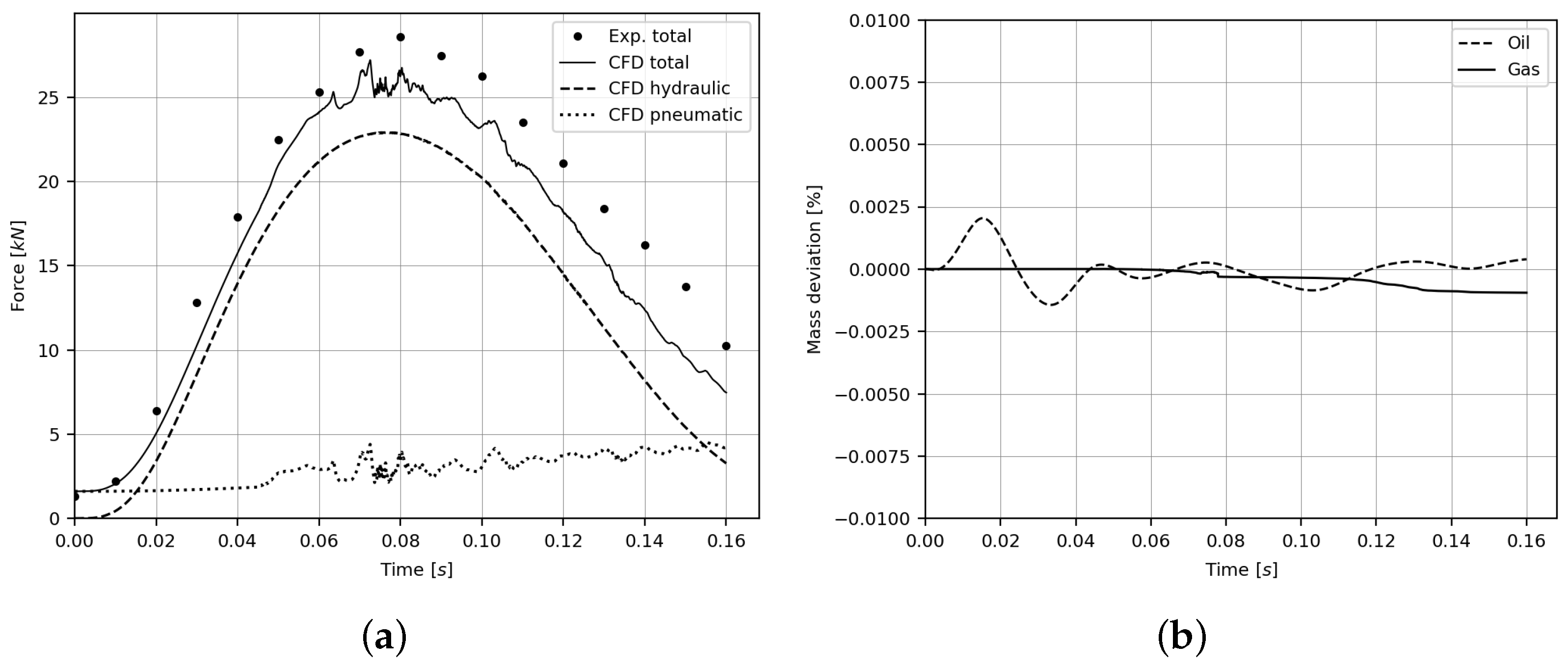
4.1. Case Validation

The validation of the drop test case is performed against the available experimental data [3], which consist of the measured total force exerted by the shock absorber in the time span from impact at 0.0 s to the end of the main stroke at 0.16 s. The total force calculated from the present simulation is compared with the experimental measurements in Figure 4a, where the agreement is found to be strong in the first half of the stroke until roughly the maximum force point, after which there is a nearly constant underprediction of the total force by the computational simulation relative to the experimental measurements. The observed discrepancy in the advanced stages of the stroke is not surprising due to the increasing complexity of the flow physics and the likely impact of simplifying assumptions.

It is worth noting that the total force cannot be extracted directly from the simulation in the manner of an accelerometer that can record the total force in the drop test. Instead, the hydraulic and pneumatic forces are computed separately and then added to arrive at the total force values [3]. The individual curves of the pneumatic and hydraulic forces are also plotted in Figure 4a to provide an insight into their contribution to the total and ensure that their overall shape and values are reasonable. The pneumatic force is calculated using averaged pressure values over the top wall of the shock absorber, accounting for the fact that the jet through the orifice impacts the central portion of the upper wall and also accounting for the strong unsteadiness in the circulating flow reaching the top of the shock absorber. The pneumatic pressure plot follows the approximate shape of the theoretical pressure increase expected for an ideal gas under compression.

The hydraulic force, on the other hand, is less straightforward to determine [10]. As it cannot be directly measured from the available parameters in simulations, it is rather calculated using Equation (1), following Ding et al. [10].

$$F_h=\rho \frac{A_h^3}{2C_D^2{A}_0^2}\dot{s}\left|\dot{s}\right|,$$

(1)

where $A_h$ is the hydraulic area, $C_D$ is the discharge coefficient, $A_0$ is the orifice area, and $|\dot{s}|$ is the stroke rate or inlet velocity in the case of the static mesh in the present simulation. This formula shows that the total force is highly dependent on the stroke rate, which is additionally demonstrated through the shape similarity between the hydraulic force curve in Figure 4a and the shapes of the inlet and orifice velocity curves shown in Figure 5.

In addition, the discharge coefficient $C_D$ is an influential parameter in the hydraulic force calculation. It is calculated using its definition in Equation (2).

$$C_D=\frac{Q_{experimental}}{Q_{theoretical}}=\frac{\dot{m}}{\rho A_0{u}_{max}},$$

(2)

where $\dot{m}$ is the mass flow through the orifice, and $u_{max}$ is the maximum velocity at the point of venna contracta, downstream of the orifice. The maximum velocity is taken as the maximum value from a series of probes placed downstream of the orifice because the position of the venna contracta depends on fluid velocity through the orifice. The maximum orifice velocity values are plotted in Figure 5.

The conservation of mass in the upper chamber is inspected for each phase. The initial quantities of gas and oil are known from experimental data. The amount of gas in the simulation remains constant, and the oil mass addition to the system can be obtained through the applied stroke rate at the inlet and the conservation of mass equation. These values are compared with the respective quantities of each phase present in the simulation as it progresses. Small mass fluctuations are seen in Figure 4b as slight deviations of simulated values from expected levels.

Oil variations are greater at the beginning and could be partially attributed to deviations from the interpolated stroke rate due to the relatively large time steps taken by the CFL-controlled adaptive time stepping when the flow is still calm. Conversely, the gas mass conservation error steadily increases as gas and oil mix vigorously, producing dispersed small gas bubbles. One potential cause of gas mass decrease is cumulative interface position calculation errors, which are more evident when phases are thoroughly mixed, resulting in a longer interface. However, the overall change in mass towards the end of the simulation is less than 0.001% of the original values and does not exceed 0.0025% at any point. Further error reduction could be achieved through grid refinement in the upper chamber, if it were deemed necessary. However, it is small enough to be considered insignificant for the purposes of the current study.

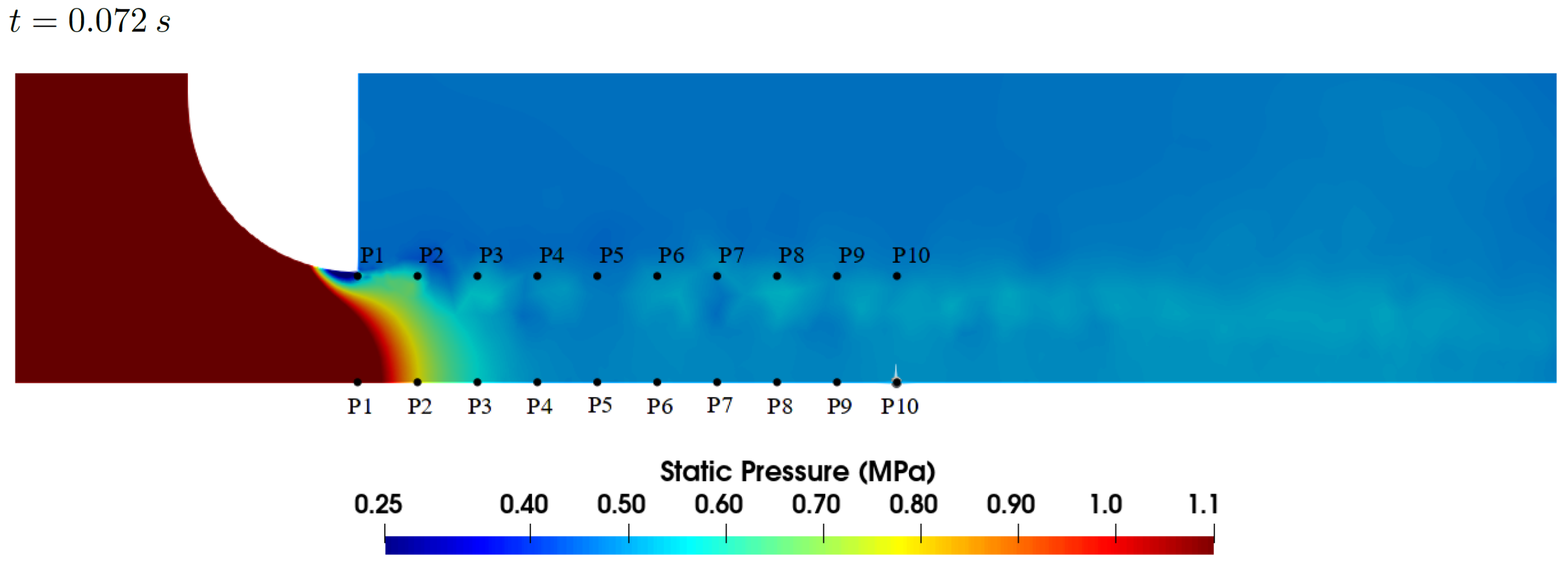
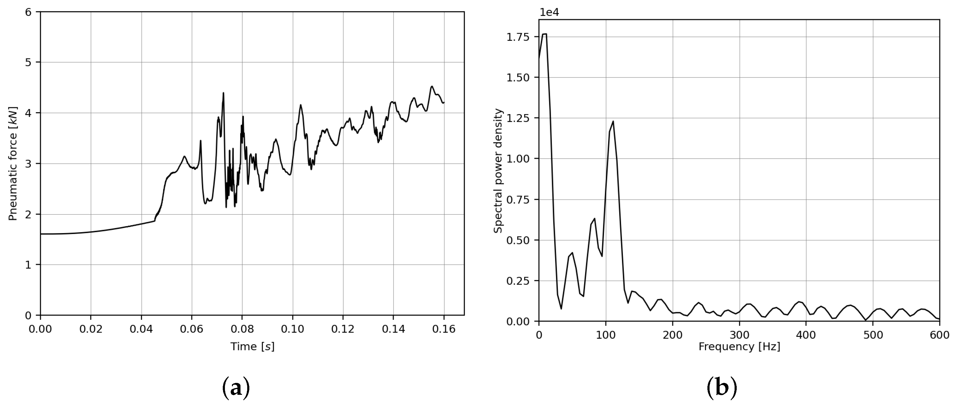
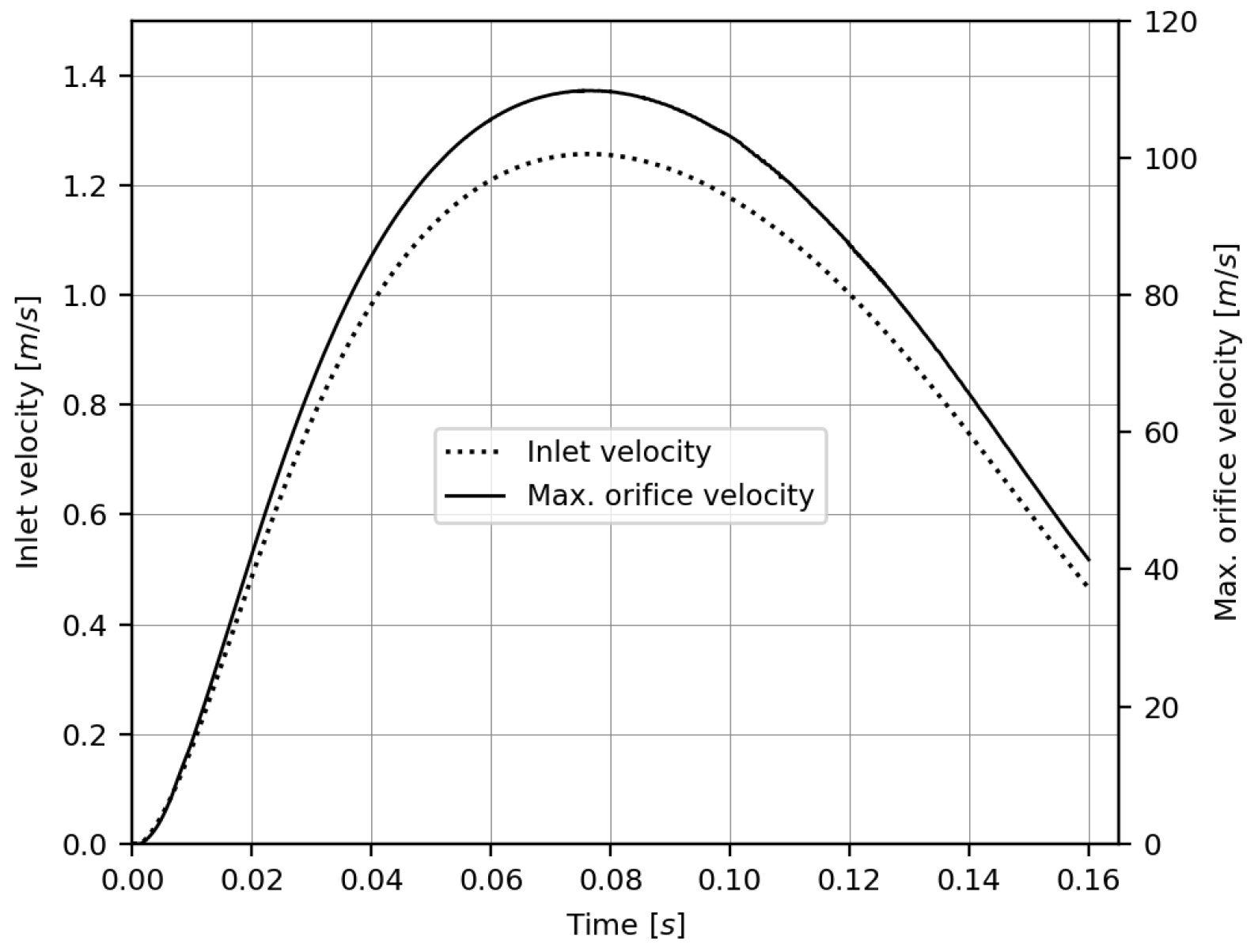
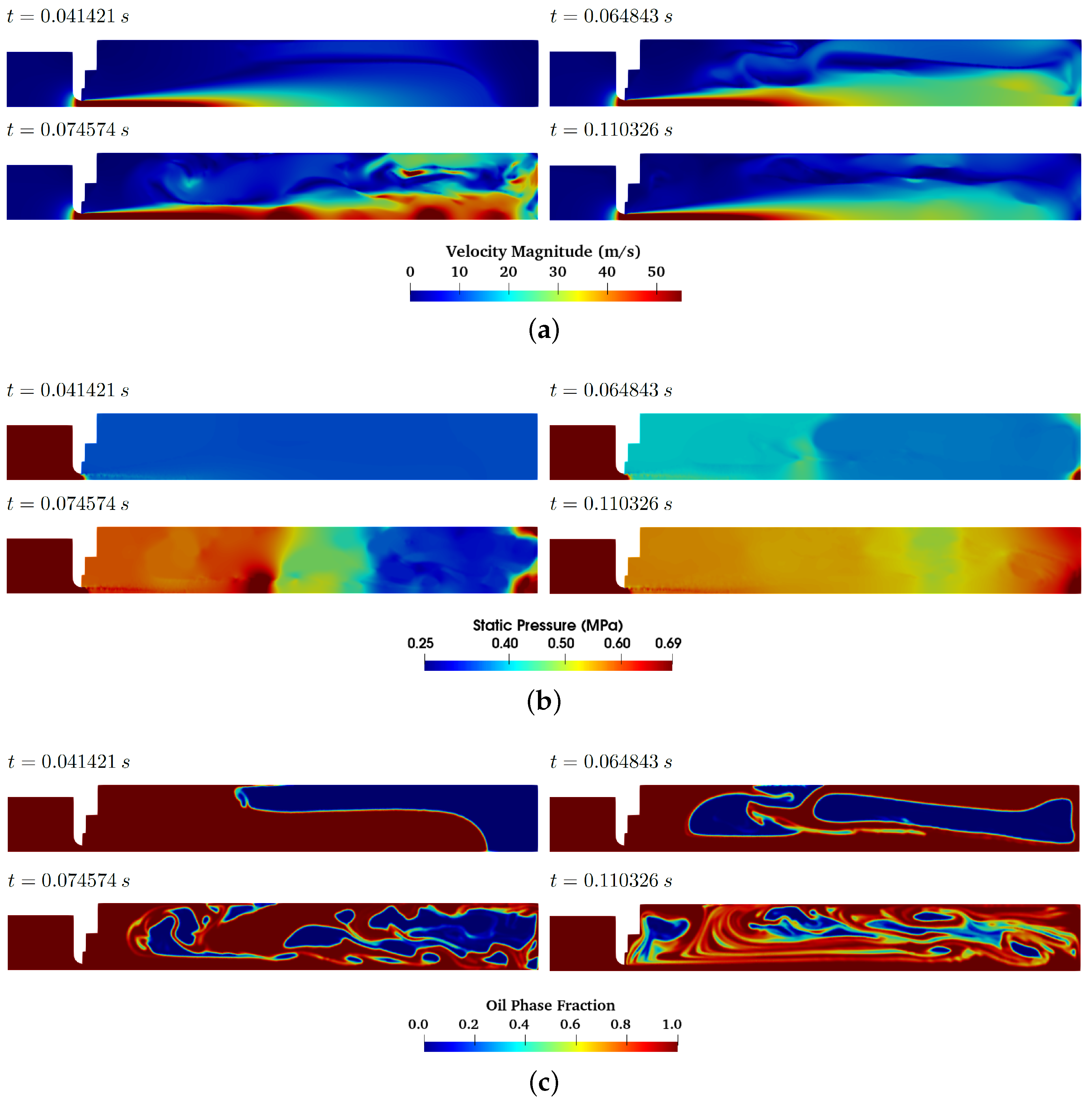
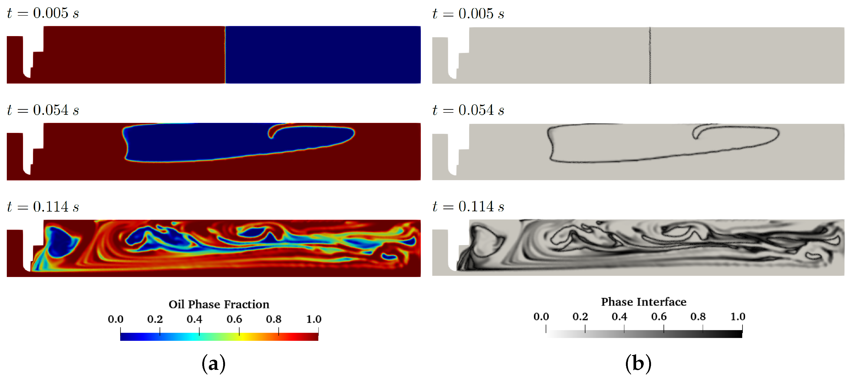
4.2. Shock Absorber Internal Flow Field Development

The shock absorber simulation is initialised with oil and gas completely separated, with the gas on top of the oil and in free contact in the upper chamber. Contour plots at four time values along the stroke are displayed in Figure 6, showing the development of velocity magnitude, oil phase fraction, and static pressure with stroke.

The simulated drop down impact on the shock absorber forces the oil through the orifice plate with strong acceleration of the fluid passing through the orifice, as can be seen from the velocity magnitude contours in Figure 6a. The jet rising through the orifice protrudes into the initially quiescent fluid in the upper chamber, generating a mixing layer along the perimeter of the jet around the potential core. This mixing layer grows laterally as the jet develops in the streamwise direction under the influence of the strong primary instability caused by the discontinuity in the velocity profile, expanding the region of high turbulence intensity towards the axis of symmetry until it closes the potential core around five orifice diameters downstream of the orifice exit. The nearfield flow development is generally consistent with the development observed in the scale resolving LES results [5]. The point of maximum velocity is found slightly downstream of the orifice along the axis at the point of vena contracta, while the velocity along the axis decreases as it approaches the upper chamber ceiling.

The confined, closed geometry of the upper chamber becomes an increasingly dominant factor in flow development as the stroke progresses. The central jet impacts the upper wall and is redirected towards the sidewalls, creating a large recirculating region extending along the entire upper chamber length. The recirculating flow interacts with the main jet, causing large-scale fluctuations of the main jet flow that become more severe as they approach the maximum stroke rate values, as seen from the plot at time t = 0.075 s in Figure 6a. However, these large-scale velocity fluctuations become weaker as the stroke rate decreases towards the final stage of the stroke at time t = 0.11 s. The free shear layer development in space and time is of interest in shock absorber simulations because the majority of the impact energy is dissipated through hydraulic resistance in the turbulent flow downstream of the orifice [2,3,4]. The changing structure of the velocity field observed in Figure 6a could be further investigated in full 3D-scale resolving simulations by applying spacial spectral analysis [38] to identify the critical regions for energy dissipation at different times along the stroke.

The static pressure contours, presented in Figure 6b, are consistent with the development observed in other flow variables. A pressure drop occurs across the orifice in all cases, as expected. Initially, the pressure in the upper chamber is relatively uniform at the beginning of the stroke at t = 0.041 s. However, strong fluctuations develop as the maximum stroke rate is approached around time t = 0.075 s, as observed with the velocity magnitude field in Figure 6a. Pressure fluctuations also become weaker towards the end of the stoke. However, the pressure in the upper chamber remains considerably less uniform than at the beginning of the stroke. It is noteworthy that the pressure near the axis of symmetry on the upper wall shows a local maxima due to the impact of the jet hitting the upper wall and becoming diverted towards the side walls. This indicates that variations in jet area or properties are likely to have a significant impact on the force felt on the upper shock absorber wall.

The oil phase fraction contour plots in Figure 6c reflect the flow development discussed above. The jet through the main orifice accelerates the hydraulic oil from the lower chamber and through the main orifice towards the upper wall of the shock absorber, which is seen to reach the top wall at approximately t = 0.041 s. This effectively forces the gas away from the top of the upper chamber towards the side wall, with it initially remaining in a single bubble; however, the violently circulating oil breaks the main gas bubble into increasingly smaller bubbles as the stroke develops. This unsteady two-phase vortex shares some similarities in its initial development with overturning water waves after impacting an obstacle in dam-break flows [20,21,22]; however, the interaction in OPSAs has a distinctive periodic character due to the confined circulating flow and persistent jet through the orifice during the stroke. It is particularly interesting to note the interaction between the gas bubbles and the free shear layer (the mixing layer) just downstream of the orifice. The larger gas bubbles break down into smaller ones on contact with the highly unsteady edge of the jet and are convected downstream with the jet, as can be seen clearly in Figure 6c at time t = 0.075 s. Furthermore, this interaction between the gas bubbles and the jet strongly corresponds to the jet’s large-scale fluctuations observed in the velocity magnitude contours in Figure 6a. As the stroke rate decreases towards the end of the stroke, time t = 0.11 s in Figure 6c, traces of the interaction between the gas bubbles and the main jet remain visible, and there is also the appearance of lower activity areas where the gas is observed to agglomerate into a slightly larger bubble, as seen around the far corner of the orifice, where there is a relatively large bubble of gas circulating in the dead-flow region. This bubble also periodically feeds gas into the oil jet as it exits the orifice.

The complexity of the interaction between the oil and gas observed in Figure 6c highlights the need for a quantitative approach to systematically assess the multiphase mixing as the stroke progresses from a straight line interface initially, shown in Figure 7a, advancing towards its full complexity as the gas bubble breaks into smaller ones. Slightly different variations in a mixing quality parameter were proposed in the literature to quantify mixing processes [39,40,41]. A similar idea is implemented here, where the mixing index (MI) in the present study, defined according to Equation (3), is used to isolate the interface between the two phases at a specific volume fraction value, taken to be $\alpha =0.5$ in all MI analyses presented.

$$MI=\mathrm{\Sigma }(1-\sqrt{{(2\alpha -1)}^2})$$

(3)

where the MI has a value of $1.0$ when $\alpha =0.5$, indicating an interface cell, while $MI=0$ when $\alpha =0$ or 1, corresponding to a cell with only a single phase. The utility of the MI as a method of isolating the interface between the phases is demonstrated in Figure 7b, where it clearly captures the developing complexity of the interaction. Furthermore, a measure of the interface area (length in 2D) can be obtained by multiplying the MI value by the local cell area (per unit depth in 2D simulations).

The interface area between the two phases corresponding to the drop test case is plotted in Figure 8. The initial value is zero because the initialisation of the two phases splits the domain into two perfectly defined regions ($\alpha =0$ or $\alpha =1$) with an instantaneous transition between the oil and gas phases. However, the full range of $\alpha$ values develops immediately after the simulation begins. A few distinctive stages of the phase mixing process can be identified and linked with the field development seen in the contour plots of Figure 6:

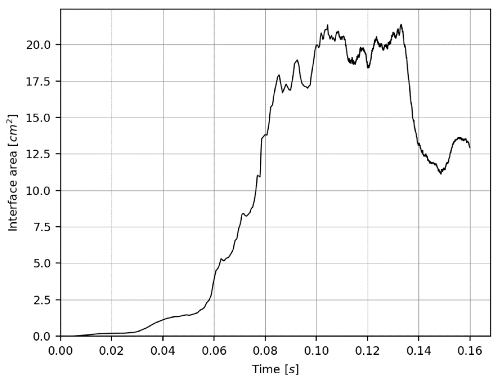
• Initial slow increase in interface area while the gas remains mainly in a single bubble, which continues until approximately t = 0.06 s in the present drop test simulation;
• A sharp increase in interface area after the main bubble starts breaking up into smaller ones over the highest stroke rate values between t = 0.06 s and t = 0.1 s;
• An approximate plateau of fluctuating values around a roughly steady interface area value, extending from t = 0.1 s to t = 0.135 s;
• A sharp decrease in interface area towards the end of the stroke, beyond t = 0.135 s, probably caused by the agglomeration of the gas into larger bubbles as the stroke rate decreases and the flow begins to settle again.

Cavitation is another important phenomenon linked to the pressure field. It occurs when the static pressure falls below a critical value, depending on the type of cavitation [42,43], leading to the formation of incipient gas bubbles that grow in low pressure regions and are then convected to higher-pressure regions, where they could violently collapse, leading to the formation of shock waves that apply high stresses on nearby surfaces. Thus, cavitation often adversely impacts the operational life span of internal components. While cavitation modelling is beyond the scope of the present work, it is possible to monitor the potential for its occurrence and to identify the regions that are most susceptible to it. Probes are placed along the orifice exit line and along the axis of symmetry, as marked in Figure 9, to assist in monitoring the flow parameters in the vicinity of the orifice over the stroke duration. Ten probes are placed on the axis of symmetry, and ten probes along the orifice tip in the downstream direction. The probe’s coordinate system origin is taken to be on the axis of symmetry line at the intersection with the orifice exit plane. The probes are uniformly distributed in the downstream direction between x = 0 m and x = 0.018 m, giving a separation between them of $\delta x$ = 0.002 m.

The static pressure contours around the orifice at approximately the maximum stroke rate, t = 0.072 s, are shown in Figure 9. The pressure falls on the orifice lip surface as the stream lines follow the curvature of its semi-circular geometry, leading to a low pressure point near the tip of the orifice at the orifice exit plane. This is consistent with the previous LES simulation of the orifice nearfield [5] and the pressure gradient contours around the orifice investigated in that study.

The P1 probes record the static pressure at the orifice tip and on the axis at the orifice exit. The general shape of the pressure history on the axis probe in Figure 10a is closely coupled to the velocity acceleration and then deceleration, corresponding to the drop test’s stroke rate profile. On the other hand, the probe at the orifice tip, in Figure 10a, records the gradual rise in pressure due to the general compression experienced in the upper chamber during the stoke, as this probe falls just outside the jet rising through the orifice. Despite the difference in the general trend, both probe plots in Figure 10a share important similarities. High-frequency oscillations abruptly appear at t = 0.06 s, which roughly corresponds to the breakup of the main gas bubble observed in Figure 6c and Figure 7a. After that, a periodic fluctuation develops at both probes, with a high amplitude peak around the maximum stroke rate time value.

Although the overall trend of static pressure values at P1 probes was observed to increase in Figure 10a, the minimum pressure on the orifice surface, slightly upstream of the orifice tip, is plotted in Figure 10b. The pressure there decreases significantly during the stroke, indicating the potential for cavitation near the orifice surface. The sharp drop and recovery of pressure values at minima hints at the possibility of violent cavitation bubble collapse when local pressure values increase sharply. This tendency towards cavitation is likely to become more significant when the loading is increased on the shock absorber or when the internal orifice design generates higher streamline curvature around the orifice, e.g., due to a sharp leading edge on the orifice. Having detected the potential for cavitation in the drop test simulated here, it is possible to conduct further studies with a suitable cavitation model [44] or use a high-order specialised code [45] to focus on cavitation in a high-fidelity study of cavitation physics using realistic boundary conditions from the unsteady shock absorber simulation.

The pneumatic force presented in Figure 4a is part of the validation discussion. It is isolated in Figure 11a for clarity. The average pressure recorded on the upper shock absorber wall also rises smoothly until the start of the gas bubble breakup process, at which point a clear periodic pattern develops. The dominant features and structure of the pneumatic force can be further investigated by taking its fast Fourier transform (FFT), as shown in Figure 11b. The FFT plot confirms that there are two dominant frequencies. The main low frequency with the highest amplitude is the stroke frequency, which provides the underlying compressive force driving the internal flow. The second highest amplitude peak is at a frequency of approximately $f\approx 110$, which corresponds to the frequency of the periodic fluctuations observed in the pneumatic force history after the time corresponding to the breakup of the gas bubble and the appearance of large-scale instabilities in the contour plots in Figure 6. These are strongly connected to the multiphase interaction and the circulation developing in the upper chamber that convects small gas bubbles in the shear layer from the recirculation region towards the upper wall. While there are some higher frequencies that appear in the pneumatic force plot, Figure 11a, it is seen in the FFT plot, Figure 11b, that they have no further dominant frequencies beyond $f\approx 110$ and appear to have a less significant impact overall. It must be noted that the signal analysed here is the time history of the averaged pressure over the shock absorber’s upper wall, where this spatial averaging process might hide some local variations. Nevertheless, the dominant features are not expected to be significantly affected.

An important feature of Figure 11b is that it confirms the dominance of relatively low frequencies in the mean flow variation, reflected in the pneumatic force signal. This implies the presence of a spectral gap between the mean flow field fluctuations and the frequencies of the turbulent flow modelled by the RANS model, which is an important consideration for the suitability of an unsteady RANS approach [30,31,32].

5. Conclusions

A multiphase oleo-pneumatic shock absorber simulation was conducted to investigate the internal dynamics of the shock absorber in a drop test case study. The results were validated against experimental measurements by Milwitzky and Cook [3].

The challenging nature of the internal shock absorber dynamics is accentuated by the lack of public validation data and geometry parameters to accurately model the internal components. This leaves many internal details, particularly in three-dimensional cases, to be estimated when reconstructing the shock absorber geometry. The simplified geometry used in the present study facilitated the identification of the main elements of internal multiphase interaction under realistic drop test boundary conditions.

Multiphase mixing was observed to progress through distinctive stages as the shock absorber stroke progressed. The initial jet through the main orifice caused a large recirculation region to develop in the upper chamber, engulfing the gas and causing the main gas bubble to break up into smaller ones with a sharp rise in the interface area between the oil and gas phases. After reaching the maximum stroke rate point, the interface area continued around roughly a plateau, with prominent fluctuations as the stoke rate decreased, until a sharp fall was observed towards the end of the stroke, probably linked to the agglomeration of gas into larger bubbles as the internal motion started settling.

Including further geometry details in the upper chamber, such as a snubber chamber, telescoping bearings, orifice support tubes, etc., will probably not affect the overall qualitative observations made in the present work, although the precise characteristics of the captured interaction and features might show some dependency on internal details. For example, the gas bubble breakup might be exacerbated by more complex internal components. This is an area that could be further investigated in future work to quantify the impact of these simplifications.

Finally, this work provided new insights into the multiphase–turbulence flow interaction influencing the dynamics and performance of OPSA systems at different stages during the stroke, thus facilitating the development of more accurate system-level models that can predict performance over a wider range of conditions.

References

1. Young, D. Aircraft landing gears—The past, present and future. Proc. Inst. Mech. Eng. Part D Transp. Eng. 1986, 200, 75–92. [Google Scholar] [CrossRef]
2. Currey, N. Aircraft Landing Gear Design: Principles and Practices; AIAA Education Series; American Institute of Aeronautics and Astronautics: Reston, VA, USA, 1988. [Google Scholar]
3. Milwitzky, B.; Cook, F.E. Analysis of Landing-gear Behavior. NACA Tech. Rept No. NACA-TR-1154. 1952. Available online: https://ntrs.nasa.gov/citations/19930092181 (accessed on 13 December 2023).
4. Schmidt, R.K. The Design of Aircraft Landing Gear; SAE International: Warrendale, PA, USA, 2021. [Google Scholar]
5. Sheikh Al-Shabab, A.A.; Grenko, B.; Vitlaris, D.; Tsoutsanis, P.; Antoniadis, A.F.; Skote, M. Numerical Investigation of Orifice Nearfield Flow Development in Oleo-Pneumatic Shock Absorbers. Fluids 2022, 7, 54. [Google Scholar] [CrossRef]
6. Daniels, J.N. A Method for Landing Gear Modeling and Simulation with Experimental Validation. NASA Rept. No. NASA-CR-201601. 1996. Available online: https://ntrs.nasa.gov/citations/19960049759 (accessed on 13 December 2023).
7. Horta, L.G.; Daugherty, R.H.; Martinson, V.J. Modeling and Validation of a Navy A6-Intruder Actively Controlled Landing Gear System. NASA Tech. Pub. No. NASA/TP-1999-209124. 1999. Available online: https://ntrs.nasa.gov/citations/19990046416 (accessed on 13 December 2023).
8. Heininen, A.; Aaltonen, J.; Koskinen, K.; Huitula, J. Equations of State in Fighter Aircraft Oleo-pneumatic Shock Absorber Modelling. Linköping Electron. Conf. Proc. 2019, 162, 64–70. [Google Scholar] [CrossRef]
9. Shi, F.; Dean, W.I.A.; Suyama, T. Single-objective Optimization of Passive Shock Absorber for Landing Gear. Am. J. Mech. Eng. 2019, 7, 107–115. [Google Scholar] [CrossRef]
10. Ding, Y.W.; Wei, X.H.; Nie, H.; Li, Y.P. Discharge coefficient calculation method of landing gear shock absorber and its influence on drop dynamics. J. Vibroengineering 2018, 20, 2550–2562. [Google Scholar] [CrossRef]
11. Du, S.; Zhang, C.; Zhou, K.; Zhao, Z. Study of the Two-Phase Flow Characteristics of a Damping Orifice in an Oleo-Pneumatic Shock Absorber. Fluids 2022, 7, 360. [Google Scholar] [CrossRef]
12. Kharangate, C.R.; Mudawar, I. Review of computational studies on boiling and condensation. Int. J. Heat Mass Transf. 2017, 108, 1164–1196. [Google Scholar] [CrossRef]
13. Mohammed, H.I.; Giddings, D.; Walker, G.S. CFD simulation of a concentrated salt nanofluid flow boiling in a rectangular tube. Int. J. Heat Mass Transf. 2018, 125, 218–228. [Google Scholar] [CrossRef]
14. Pothukuchi, H.; Kelm, S.; Patnaik, B.; Prasad, B.; Allelein, H.J. CFD modeling of critical heat flux in flow boiling: Validation and assessment of closure models. Appl. Therm. Eng. 2019, 150, 651–665. [Google Scholar] [CrossRef]
15. Mulbah, C.; Kang, C.; Mao, N.; Zhang, W.; Shaikh, A.R.; Teng, S. A review of VOF methods for simulating bubble dynamics. Prog. Nucl. Energy 2022, 154, 104478. [Google Scholar] [CrossRef]
16. Vaishnavi, G.S.; Ramarajan, J.; Jayavel, S. Numerical studies of bubble formation dynamics in gas-liquid interaction using Volume of Fluid (VOF) method. Therm. Sci. Eng. Prog. 2023, 39, 101718. [Google Scholar] [CrossRef]
17. Rabha, S.S.; Buwa, V.V. Volume-of-fluid (VOF) simulations of rise of single/multiple bubbles in sheared liquids. Chem. Eng. Sci. 2010, 65, 527–537. [Google Scholar] [CrossRef]
18. Lahey, R.T., Jr.; Baglietto, E.; Bolotnov, I.A. Progress in multiphase computational fluid dynamics. Nucl. Eng. Des. 2021, 374, 111018. [Google Scholar] [CrossRef]
19. Lauber, G.; Hager, W.H. Experiments to dambreak wave: Horizontal channel. J. Hydraul. Res. 1998, 36, 291–307. [Google Scholar] [CrossRef]
20. Stansby, P.; Chegini, A.; Barnes, T. The initial stages of dam-break flow. J. Fluid Mech. 1998, 374, 407–424. [Google Scholar] [CrossRef]
21. Tan, T.; Ma, Y.; Zhang, J.; Niu, X.; Chang, K.A. Experimental study on flow kinematics of dam-break induced surge impacting onto a vertical wall. Phys. Fluids 2023, 35, 025127. [Google Scholar] [CrossRef]
22. Issakhov, A.; Zhandaulet, Y.; Nogaeva, A. Numerical simulation of dam break flow for various forms of the obstacle by VOF method. Int. J. Multiph. Flow 2018, 109, 191–206. [Google Scholar] [CrossRef]
23. Abdolmaleki, K.; Thiagarajan, K.; Morris-Thomas, M. Simulation of the dam break problem and impact flows using a Navier-Stokes solver. Simulation 2004, 13, 17. [Google Scholar]
24. Zhainakov, A.Z.; Kurbanaliev, A. Verification of the open package OpenFOAM on dam break problems. Thermophys. Aerom. 2013, 20, 451–461. [Google Scholar] [CrossRef]
25. Besagni, G.; Varallo, N.; Mereu, R. Computational Fluid Dynamics Modelling of Two-Phase Bubble Columns: A Comprehensive Review. Fluids 2023, 8, 91. [Google Scholar] [CrossRef]
26. Besagni, G.; Inzoli, F.; Ziegenhein, T. Two-phase bubble columns: A comprehensive review. ChemEngineering 2018, 2, 13. [Google Scholar] [CrossRef]
27. Al-Shabab, A.A.S.; Tucker, P.G. Toward Active Computational Fluid Dynamics Role in Open Jet Airfoil Experiments Design. AIAA J. 2018, 56, 3205–3215. [Google Scholar] [CrossRef]
28. Al-Shabab, A.S.; Tucker, P. RANS prediction of open jet aerofoil interaction and design metrics. Aeronaut. J. 2019, 123, 1275–1296. [Google Scholar] [CrossRef]
29. Sheikh-AlShabab, A.A.; Tucker, P.G. Numerical Investigation of Installation Effects in Open Jet Wind Tunnel Airfoil Experiments. In Proceedings of the 52nd Aerospace Sciences Meeting, AIAA Paper, National Harbor, MD, USA, 13–17 January 2014. [Google Scholar] [CrossRef]
30. Tucker, P. Computation of unsteady turbomachinery flows: Part 1—Progress and challenges. Prog. Aerosp. Sci. 2011, 47, 522–545. [Google Scholar] [CrossRef]
31. Tucker, P. Computation of unsteady turbomachinery flows: Part 2—LES and hybrids. Prog. Aerosp. Sci. 2011, 47, 546–569. [Google Scholar] [CrossRef]
32. Tucker, P. Trends in turbomachinery turbulence treatments. Prog. Aerosp. Sci. 2013, 63, 1–32. [Google Scholar] [CrossRef]
33. Sheikh Al Shabab, A.; Grenko, B.; Vitlaris, D.; Tsoutsanis, P.; Antoniadis, A.; Skote, M. Numerical investigation of oleo-pneumatic shock absorber: A multi-fidelity approach. In Proceedings of the ECCOMAS Congress 2022—8th European Congress on Computational Methods in Applied Sciences and Engineering, ECCOMAS, Oslo, Norway, 5–9 June 2022. [Google Scholar] [CrossRef]
34. ANSYS Fluent. Release 2019 R2, Theory Guide; ANSYS Inc.: Southpoint, Canonsburg, PA, USA, 2019. [Google Scholar]
35. Menter, F.R. Two-equation eddy-viscosity turbulence models for engineering applications. AIAA J. 1994, 32, 1598–1605. [Google Scholar] [CrossRef]
36. Menter, F.R.; Kuntz, M.; Langtry, R. Ten years of industrial experience with the SST turbulence model. Turbul. Heat Mass Transf. 2003, 4, 625–632. [Google Scholar]
37. Menter, F.R. Review of the shear-stress transport turbulence model experience from an industrial perspective. Int. J. Comput. Fluid Dyn. 2009, 23, 305–316. [Google Scholar] [CrossRef]
38. Tsoutsanis, P.; Nogueira, X.; Fu, L. A short note on a 3D spectral analysis for turbulent flows on unstructured meshes. J. Comput. Phys. 2023, 474, 111804. [Google Scholar] [CrossRef]
39. Solehati, N.; Bae, J.; Sasmito, A.P. Numerical investigation of mixing performance in microchannel T-junction with wavy structure. Comput. Fluids 2014, 96, 10–19. [Google Scholar] [CrossRef]
40. Wang, S.; Huang, X.; Yang, C. Mixing enhancement for high viscous fluids in a microfluidic chamber. Lab Chip 2011, 11, 2081–2087. [Google Scholar] [CrossRef] [PubMed]
41. Nguyen, Q.; Papavassiliou, D.V. Quality Measures of Mixing in Turbulent Flow and Effects of Molecular Diffusivity. Fluids 2018, 3, 53. [Google Scholar] [CrossRef]
42. Yan, Y.; Thorpe, R. Flow regime transitions due to cavitation in the flow through an orifice. Int. J. Multiph. Flow 1990, 16, 1023–1045. [Google Scholar] [CrossRef]
43. Osterland, S.; Günther, L.; Weber, J. Experiments and Computational Fluid Dynamics on Vapor and Gas Cavitation for Oil Hydraulics. Chem. Eng. Technol. 2023, 46, 147–157. [Google Scholar] [CrossRef]
44. Folden, T.S.; Aschmoneit, F.J. A classification and review of cavitation models with an emphasis on physical aspects of cavitation. Phys. Fluids 2023, 35, 081301. [Google Scholar] [CrossRef]
45. Antoniadis, A.F.; Drikakis, D.; Farmakis, P.S.; Fu, L.; Kokkinakis, I.; Nogueira, X.; Silva, P.A.; Skote, M.; Titarev, V.; Tsoutsanis, P. UCNS3D: An open-source high-order finite-volume unstructured CFD solver. Comput. Phys. Commun. 2022, 279, 108453. [Google Scholar] [CrossRef]
Figure 1. Schematic view of the simplified shock absorber geometry.
Fluids 09 00068 g001
Figure 2. Shock absorber geometry simplification: (a) telescoping internal geometry; (b) fixed shock absorber geometry; (c) unstructured mesh used with boundary conditions.
Fluids 09 00068 g002
Figure 3. Shock absorber geometry and some setup details: (a) dynamic system model; (b) stroke rate profile calculated from the 2-DOF dynamic system model.
Fluids 09 00068 g003
Figure 4. Shock absorber case validation: (a) force validation; (b) mass conservation of the oil and gas phases.
Fluids 09 00068 g004
Figure 5. The specified inlet velocity (stroke) and the maximum orifice velocity along the axis of symmetry.
Fluids 09 00068 g005
Figure 6. Drop test contour plots at four time values along the stroke showing the internal flow field development with stroke progress. (a) Velocity magnitude; (b) static pressure; (c) oil phase fraction.
Fluids 09 00068 g006
Figure 7. Multiphase contour plots demonstrating how the mixing index can be applied to visualise the interface cells in order to quantify the mixing intensity. (a) Phase fraction; (b) Phase interface.
Fluids 09 00068 g007
Figure 8. Multiphase interface time history demonstrating the different stages of mixing and the sharp gradients that indicate the occurrence of strong mixing.
Fluids 09 00068 g008
Figure 9. Static pressure field around the orifice, with pressure data probes displayed showing the region of low pressure around the orifice.
Fluids 09 00068 g009
Figure 10. Pressure probes’ analysis plots: (a) P1 orifice and axis probe plots over time; (b) pressure over time plot at the point of greatest pressure drop, revealing the sharp pressure fall with stroke progress, creating the potential for cavitation to occur if the pressure falls far enough.
Fluids 09 00068 g010
Figure 11. Pneumatic force on upper wall showing periodic fluctuations similar to the ones observed in the data from the probes near the orifice. (a) Pneumatic force; (b) fast Fourier transform (FFT) of upper wall pneumatic force.
Fluids 09 00068 g011