Abstract
This study presents a novel approach to using a gated recurrent unit (GRU) model, a deep neural network, to predict turbulent flows in a Lagrangian framework. The emerging velocity field is predicted based on experimental data from a strained turbulent flow, which was initially a nearly homogeneous isotropic turbulent flow at the measurement area. The distorted turbulent flow has a Taylor microscale Reynolds number in the range of 100 < < 152 before creating the strain and is strained with a mean strain rate of 4 in the Y direction. The measurement is conducted in the presence of gravity consequent to the actual condition, an effect that is usually neglected and has not been investigated in most numerical studies. A Lagrangian particle tracking technique is used to extract the flow characterizations. It is used to assess the capability of the GRU model to forecast the unknown turbulent flow pattern affected by distortion and gravity using spatiotemporal input data. Using the flow track’s location (spatial) and time (temporal) highlights the model’s superiority. The suggested approach provides the possibility to predict the emerging pattern of the strained turbulent flow properties observed in many natural and artificial phenomena. In order to optimize the consumed computing, hyperparameter optimization (HPO) is used to improve the GRU model performance by 14–20%. Model training and inference run on the high-performance computing (HPC) JUWELS-BOOSTER and DEEP-DAM systems at the Jülich Supercomputing Centre, and the code speed-up on these machines is measured. The proposed model produces accurate predictions for turbulent flows in the Lagrangian view with a mean absolute error (MAE) of 0.001 and an score of 0.993.
1. Introduction
Turbulent flow is a high-dimensional and nonlinear phenomenon [1]. It can be found in many artificial and natural applications, and it is therefore of great interest to study its features [1,2,3]. All turbulent flows have random characteristics, rendering deterministic approaches impossible to apply. Therefore, existing analyses rely on statistical methods addressing the energy cascade theory [1,2]. The use of computational fluid dynamic (CFD) methods is a convenient approach for simulating turbulent flows, mainly via direct numerical simulation (DNS) and large eddy simulation (LES) [1]. Although LES is less accurate than DNS, both methods require extensive computing [4] on high-performance computing (HPC) systems. Solving Reynolds-averaged Navier Stokes (RANS) equations is a cheap method used widely in the industry, though it does not provide results on the level of accuracy of LES or DNS. The size and scalability of HPC systems is continuously growing, allowing for more and more fine-grained simulations. However, current numerical methods are far from being able to compute every CFD problem, especially those featuring highly complex and detailed flow structures [4,5]. Furthermore, in many CFD applications, a validation of the solution via empirical data is essential, which is another disadvantage [4]. Experiments are frequently used to study the turbulent flow. However, due to their scale and size limitations, they can only be applied to particular and size-limited problems [1,3,6,7]. These constraints underpin the demands for a reliable tool to overcome the obstacles mentioned above and analyze turbulent flows in a broader range of scales [4]. Several methods extract the dominant features via the reduced-order model (ROM). Proper orthogonal decomposition (POD), dynamical mode decomposition (DMD), and Koopman analyses are some of the well-known techniques to yield ROM [8]. Moreover, dimensionality reduction, feature extraction, super-resolution, applying ROM, turbulence closure, shape optimization, and flow control are some of the crucial tasks in CFD [9].
In many areas, deep learning (DL) models have demonstrated an extensive capability to extract hidden features from nonlinear events and create predictions [8,9]. The applicability of DL models has also been studied in fluid dynamics [4]. Recent studies show that with DL, model-free predictions of spatiotemporal dynamical systems, particularly for high-dimensional, dynamical systems [8], are possible. Recurrent neural networks (RNN) are neural networks composed of an individual hidden layer with a feedback loop, in which the hidden layer output and the current input are turned to the hidden layer [9]. They are well-suited for sequential datasets [9]. They determine a temporal relationship, as they learn from sequential input data and are characterized by featuring three weight metrics and two biases. However, RNN cannot learn long-range temporal dependencies from sequential data due to the vanishing gradient problem [9]. The long short-term memory (LSTM) model was developed in 1995 [10]. It features a gating structure to control the recurrent connector transients. In contrast to RNN, vanishing gradients are avoided. It is therefore a proper tool to model longer temporal dependencies [9]. Gated recurrent unit (GRU) models are variants of LSTM models that work with fewer parameters [11,12]. Besides, in GRU architectures, the forget and input gates of LSTM are altered only with one update gate. In the literature, it has been shown that GRU models can be trained faster while still achieving results similar to LSTM, even with fewer training data [12]. Duru et al. [13] apply DL to predict the transonic flow around airfoils. Srinivasan et al. [9] use Multilayer Perceptron (MLP) and DL networks to predict a turbulent shear flow from equations known from a Moehlis model [14]. LSTM’ susceptibility has led to hybrid models such as autoencoders-LSTM, LSTM/RNN, and Convolutional Neural Network (CNN)-LSTM [12]. Eivazi et al. [8] present a DL application for the nonlinear model reduction in unsteady flows. The review of Gu, Chengcheng, and Li, Hua [12] reports on an LSTM network being applied to predict the wind speed, which has turbulent behavior. Bukka et al. [5] employ a hybrid, deeply reduced model to predict unsteady flows. Most fluid flow studies that applied DL use data extracted from CFD computations [4,9]. Furthermore, most works include pre-processing steps to identify the dominant features, such as POD or DMD [4]. Recently, Hassanian et al. [15] used LSTM and GRU models to predict a turbulent flow with only temporal features. Moreover, the Transformer model, as an up-to-date DL technique, displays successful capabilities to simulate and forecast emerging unknown patterns of turbulent flow [16].
This study proposes an innovative idea, using a GRU model to predict turbulent flows with spatial-temporal data based on raw data from flow measurements in an experiment of strained turbulent flow [17]. The Lagrangian particle tracking (LPT) technique is applied to extract 2D (two components of each property, such as velocity) from the 3D experiment (consisting of all components of each property) of the strained turbulent flow. As the turbulent flow manifests as a three-dimensional phenomenon, employing experimental data yields a dataset containing authentic and comprehensive turbulence characteristics. The data contain information on the time t, location x and y, and the velocity components in the X and the Y directions. The Lagrangian framework is defined by particle traces in a spatiotemporal way [6,7]. A particle in the flow with a specific velocity and position at each particular time t is followed [1,6]. This way, the particle’s velocity over time can be represented as a time series [4], which is a function of the particle’s location. Relying on this concept, a GRU model can be trained with the spatiotemporal data and predict the velocity. The velocity time series in fluid dynamics have been recorded in several biological and industrial applications via special devices [4] and can be used in combination with the suggested model. Since the turbulent flow is a nonlinear problem and there is no deterministic approach to solve or forecast the emerging period of its feature, the suggested method in the present study provides a transparent window to study turbulent flow.
In prior research on turbulent flow employing deep learning models, a hybrid approach incorporating Proper Orthogonal Decomposition (POD), Reduced Order Modeling (ROM) [18], and deep learning techniques was employed to address nonlinear parametrized Partial Differential Equations (PDEs) [19,20]. The superiority of this proposed method is that it eliminates the steps of extracting the dominant data and the necessary pre-processing steps before the application of DL, and directly provides predictions of the future flow through DL models. This advantage renders the model adaptable for training with raw measurement data, eliminating the need for processing, such as ROM or POD. Its novelty in applying training data for a DL model is based on spatio-temporal attributes. In sequential DL models such as LSTM and GRU, the training data are times series and, therefore, temporal. The current study employs the spatial attributes of the turbulent flow since, in the Lagrangian framework, the location is a function of the time. Furthermore, the preeminence of the present study is utilizing the GRU model to be trained with measured property, forecasting it in the following period without training, and informing the model with flow characteristics such as the Reynolds number, Stokes number, length, or time scale. In many industries and applications, fluid flow properties such as velocity, flow rate, vorticity, and acceleration can be measured with technical devices. This consistency helps the proposed approach to be broadly utilized. The experimental dataset used in the present study stems from a strained turbulence flow in the presence of gravity and tracking tracer particles. However, the prediction model only relies on the velocity and location time series, and the training does not include parameters such as particle size, turbulence intensity, gravity, and strain rate. The parallel computing machines JUWELS-BOOSTER and DEEP-DAM [21] from the Jülich Supercomputer Centre are used to accelerate the GRU model training process. Hence, this manuscript is organized as follows. The applied methodology is introduced in Section 2. Subsequently, the results and discussion are provided in Section 3. Finally, conclusions are drawn in Section 4.
2. Methodology
This section represents the theory of the LPT, which is used to employ a dataset from the experiment in this study. Furthermore, the dataset details have been explained. Thus, the employed GRU model and its setup for training and prediction have been demonstrated.
2.1. The Lagrangian Framework and Fluid Particles
In a Lagrangian framework, individual fluid particles’ position and velocity vectors are tracked [1,6]. A fluid particle is a point that streams with the local flow velocity; thus, it identifies the velocity and position at time t. The arithmetic definition of a fluid particle is [1,4]:
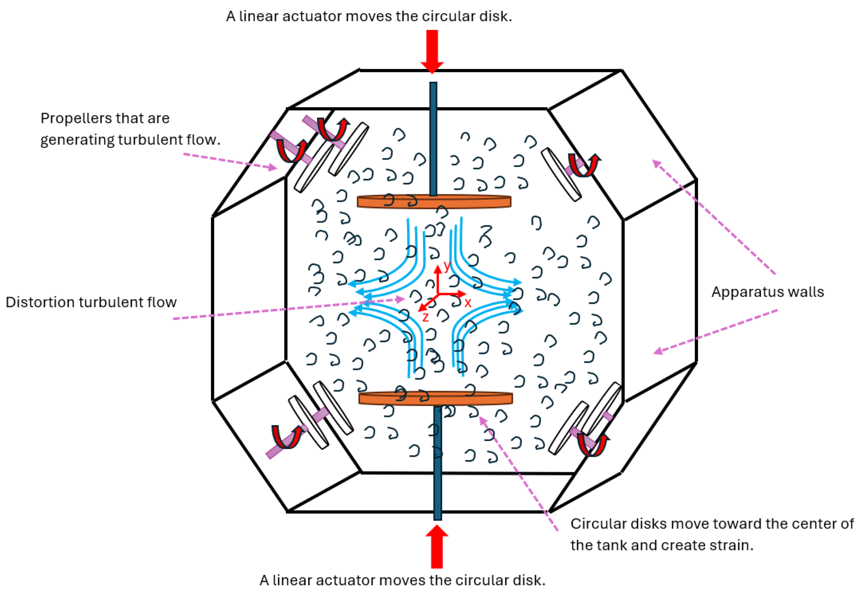
where the velocity U is determined in 3D coordinates, x is the position vector, t is the time, and i specifies the vector components in the X, the Y, and the Z directions. Notation (1) defines the particle velocity in sequential time series and is frequently used in turbulent flow statistics, where no universal velocity function is available. ascertains the initial condition of the particle in the i direction. Figure 1 displays a sketch of the strained turbulent flow.
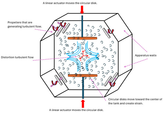
Figure 1.
A sketch displays the strain acting on the turbulent flow. The turbulent flow at the measurement area, located at the center of the tank, is a nearly stationary homogeneous isotropic turbulence flow initially and before the distortion. The measured data are used in the current study to train a GRU model.
2.2. Experimental Data
The experiment was conducted within a water tank featuring eight impellers strategically positioned at the corners of a cube and directed toward the tank’s center, as displayed in Figure 1. These impellers rotated at specific speeds falling within the range of 100 < < 152, effectively simulating the turbulent flow before creating the strain deformation. The resulting flow in the central region of the tank, where measurements were taken, exhibited a nearly stationary homogeneous isotropic turbulence [22]. The tank, with dimensions of 60 cm × 60 cm × 60 cm, had transparent Plexiglas for XT walls that were 20 mm thick, allowing optical access to the data. An aluminum frame held the components of the turbulence box in place. The fluid in the tank was seeded with tracer particles with median diameters of 8–10 . Tracer particles had a specific gravity of 1.1 (hollow glass). Two circular flat disks positioned vertically in the center of the tank moved towards each other, generating a specified mean strain rate. The experiment involved a mean strain rate, primarily in the y-direction of −4 . The measurement area, situated in the center of the tank, had dimensions of 24.5 × 24.5 .
The Lagrangian particle tracking (LPT) technique was employed to monitor and extract the dynamic features of the particles. Lagrangian Particle Tracking (LPT) [23,24,25] is a non-intrusive optical methodology that is widely utilized in experimental fluid dynamics. This technique involves capturing images of particles suspended in a fluid and subsequently tracking the movement of individual particles within a small interrogation window. In the context of two-dimensional LPT, the flow field is observed within a thin plane illuminated by a laser sheet, allowing for the measurement of particle motion within that specific slice of the flow. Introducing low-density particles into the flow of interest allows each particle to be individually tracked across multiple frames.
In this particular experiment, a single camera was utilized to reconstruct particle tracks in two dimensions, providing valuable insights into the initial turbulence and Lagrangian statistics of the turbulent flow. The construction of particle tracks in 2D-LPT involves two primary tasks. Firstly, the images captured by the camera undergo processing to determine the two-dimensional positions of the particles within the camera’s image space. Secondly, a tracking algorithm, based on the principle of the 4-frame best estimate pioneered by Ouelette et al. [25], is applied to establish the paths followed by the particles over time using a sequence of images.
A solitary high-speed CMOS camera equipped with a 105 mm focal length lens was employed to capture LPT images, set at a resolution of 512 × 512 pixels. The detection system operated at 10 kHz, equivalent to 10,000 frames per second (fps), ensuring well-resolved particle velocity and acceleration statistics. This exceptionally high temporal resolution (0.1–0.2 ms) is significantly smaller than the Kolmogorov time (16.6–31.6 ms) of the smallest eddies in the flow, allowing for the resolution of dissipation range properties. It is reported that the Stokes number (relaxation time over the Kolmogorov scale) for the tracer particles is in the range of 0.0063–0.0094 [17]. For illuminating the tracer particles; an Nd-YAF laser (527 nm) was utilized, synchronized at the same sampling frequency as the camera. The laser operated in an internal mode, with a 14 A Q-switch current and a pulse width of 2.5 . To ensure accurate statistics of the particle-laden turbulent flow, the recording process was iterated 20 times for each flow case. It is important to note that the present study uses a dataset to train a GRU model originated from the LPT measurement based on Ouelette et al. [25] and Hassanian et al. [17]. The original work [17] details the experiments and their measurements.
2.3. Sequential Velocity Dataset
The velocity dataset is extracted from the LPT experiment described in the previous section, following the procedure of Hassanian et al. [17]. The dataset is composed of 6,225,457 tracking points for every vector, as follows:
- Velocity component in the Y direction, ;
- Velocity component in the X direction, ;
- Location in the x coordinate;
- Location in the y coordinate;
- The time vector specifies the time t for every tracking point.
These tracking points comprise velocity and location vectors, attained via 20 recordings to provide sufficient statistical data. As expected, the tracking yields several tracking lines, as illustrated in the result section, and every tracking line specifies the fate of a single particle. This study employed different ratios of the training dataset to determine the optimal model with accurate predictions for the strained turbulent flow. To measure the performance of the forecasting model, the data are split into 80% training data and 20% test data. The prediction quality of the model is evaluated on the unseen test data. The model is trained in a way that individually predicts the velocity in the X direction and the Y direction. This design makes the model applicable to higher-dimensional data. For instance, if there are data with a third component in the Z direction, this model can forecast the corresponding velocity component in a separate training run. It should be noted that the dataset in this study underwent strain deformation in the Y direction, which is the dominant orientation in this flow; therefore, it is expected to see more fluctuation in this direction [3,17].
2.4. Gated Recurrent Unit Model
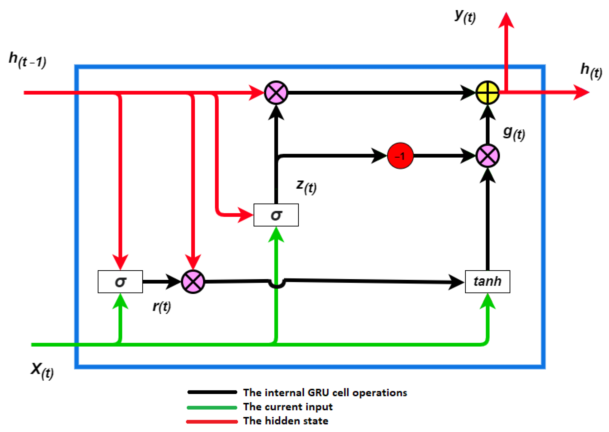
The study relies on the concept that the flow properties in the Lagrangian frameworks are carried by the velocity, which is a function of time and location. Therefore, the input data from the 2D measurement involves the location in the x and the y coordinates in addition to velocity components in both orientations. The current study trained a DL model on these data to assess the ability to forecast flow fields, because the concept of sequentiality is an inherent feature in the Lagrangian framework. The DL model thereby takes into account all historical impacts. Despite the mean strain rate, turbulence intensity, geometry of the boundary condition as an effectiveness parameter [26,27], and gravity as a presence effect [17], they are not part of the model input. The only inputs to train the model are locations and the velocity. The target is the velocity in the future. A GRU is based on the LSTM model with slight changes in the architecture [28]. The literature reports that a GRU is faster to compute than an LSTM and has a streamlined model [11,12,29]. A GRU cell, which is displayed in Figure 2, is composed of a hidden state , a reset gate , and an update gate . The reset gate controls how much of the previously hidden state is remembered. Via the update gate, it can be quantified how much of the new hidden state is just a copy of the old hidden state. This architecture establishes two significant features: the reset gate captures short-term dependencies and the update gate models’ long-term dependencies in sequences [28].

Figure 2.
Architecture of a GRU model: is the hidden state from the previous step, is the current input, is a new hidden state, is the output, is the reset gate, is the update gate, is the candidate hidden state, is the sigmoid function, and is the hyperbolic tangent function [15].
2.5. Forecasting Model Set Up and Parallel Computing
The models are coded in Python with the TensorFlow library [30,31]. The GRU model is set up with 100 layers and one dense layer, and Adam is specified as an optimizer [15]. The dataset was normalized by the MinMaxScaler transformation [32], scaling the minimum and maximum values to be 0 and 1. In the GRU model, is _, and the learning rate is 0.001. Since the model training runs on the JUWELS-BOOSTER [33] and DEEP-DAM [21] machines, a distribution strategy from the TensorFlow interface to distribute the training across multiple GPU with custom training loops is applied [34]. The training has been set up to use 1 to 4 GPU on one node. The result of the computing and the models’ performance distinction are reported in Section 3.
3. Results
The current study makes use of a dataset from an LPT measurement, which provides spatial and temporal information. The visualization of the velocity that is measured in the X and Y directions is obtained to observe the flow turbulency behavior. The velocity in a specific direction at location x and y is used as input training data with a ratio of . The velocity prediction was evaluated with the rest of the data (). The trained model performs the forecast for both velocities individually. In this section, the results and discussion are presented.
3.1. Measured Turbulent Flow Velocity
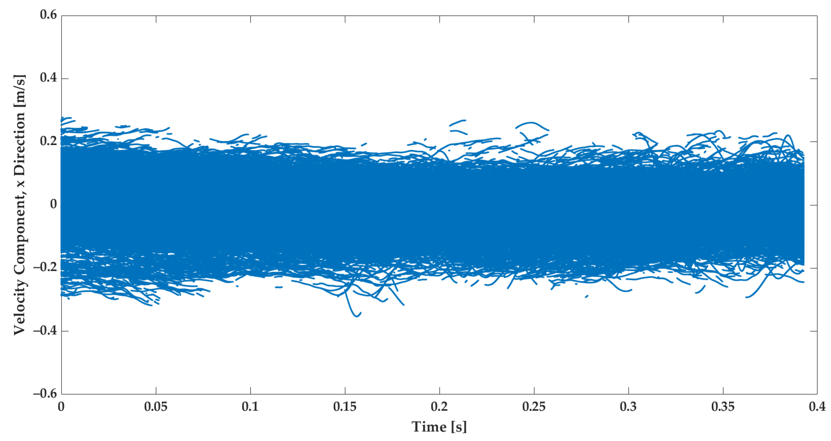
The subject of this study is to employ the dataset from the experiment in the training of the GRU model and to analyze its training and predictive performance. The data extracted from the experiments contain the velocities of tracer particles in the Lagrangian framework [17]. Figure 3 and Figure 4 illustrate the measured velocity component in the X and Y directions, respectively.
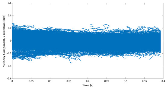
Figure 3.
The measured velocity in the X direction from 20 videos for strained turbulent flow. The experiments have been repeated in analogous conditions.
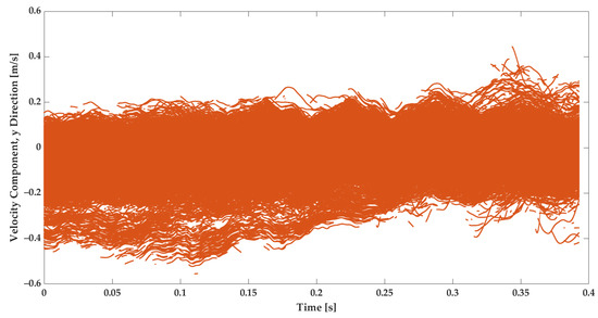
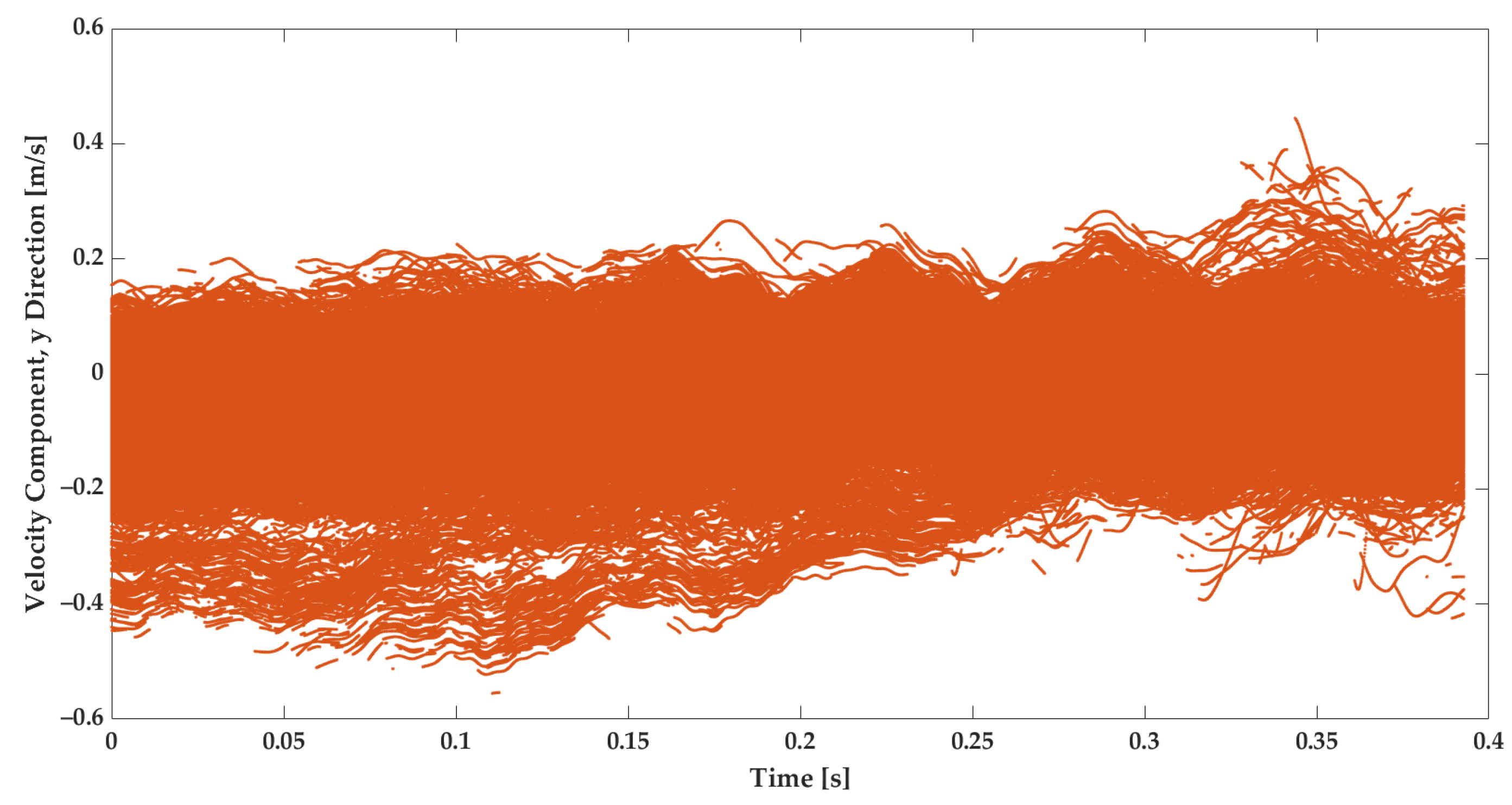
Figure 4.
The measured velocity in the Y direction from 20 videos for strained turbulent flow. The experiments have been repeated in analogous conditions.
The velocity measurements in the X and Y directions both show fluctuations. Comparing Figure 3 and Figure 4 reveals that in the Y direction, the turbulence is more intense. This is due to the fact that the strain direction mainly points to this orientation [17]. That is, the velocity in the Y direction has a gradient that is caused by the strain. It is, therefore, much more visible than the velocity in the X direction. The literature emphasizes that the strain could lead to extra fluctuations [2,3,17]. Besides the strain and turbulence intensity, the geometry boundary influences the flow velocity [3].
3.2. Predicted Velocity and GRU Model Evaluation
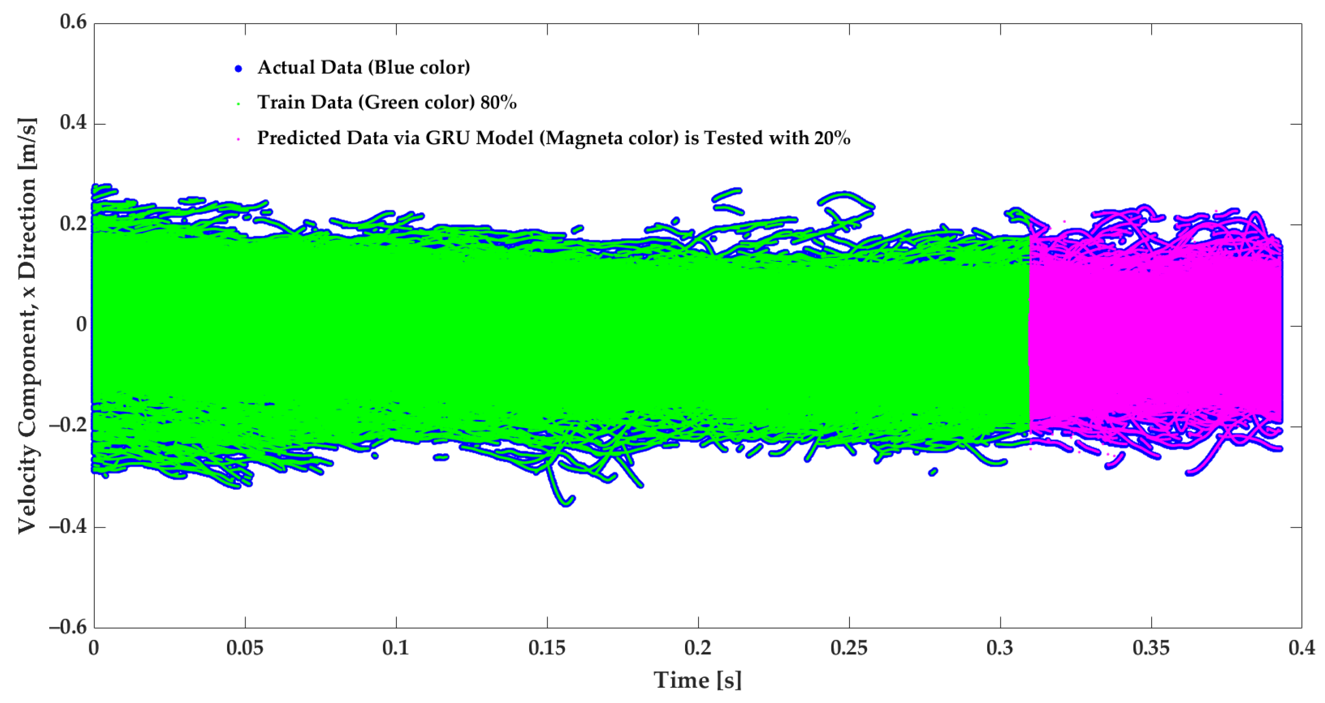
Figure 5 and Figure 6 illustrate that of the velocity time series are used to train the GRU model in this study. The rest of the data () are applied as test data to assess the predicted velocity via the GRU model.
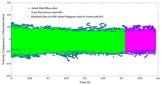
Figure 5.
Velocity prediction of the velocity in the X direction from the GRU model. The model is trained on of the data, while the remaining is used for testing. The filled blue circles are actual data, the green points are train data, and the magenta points are GRU-predicted data.
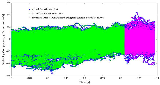
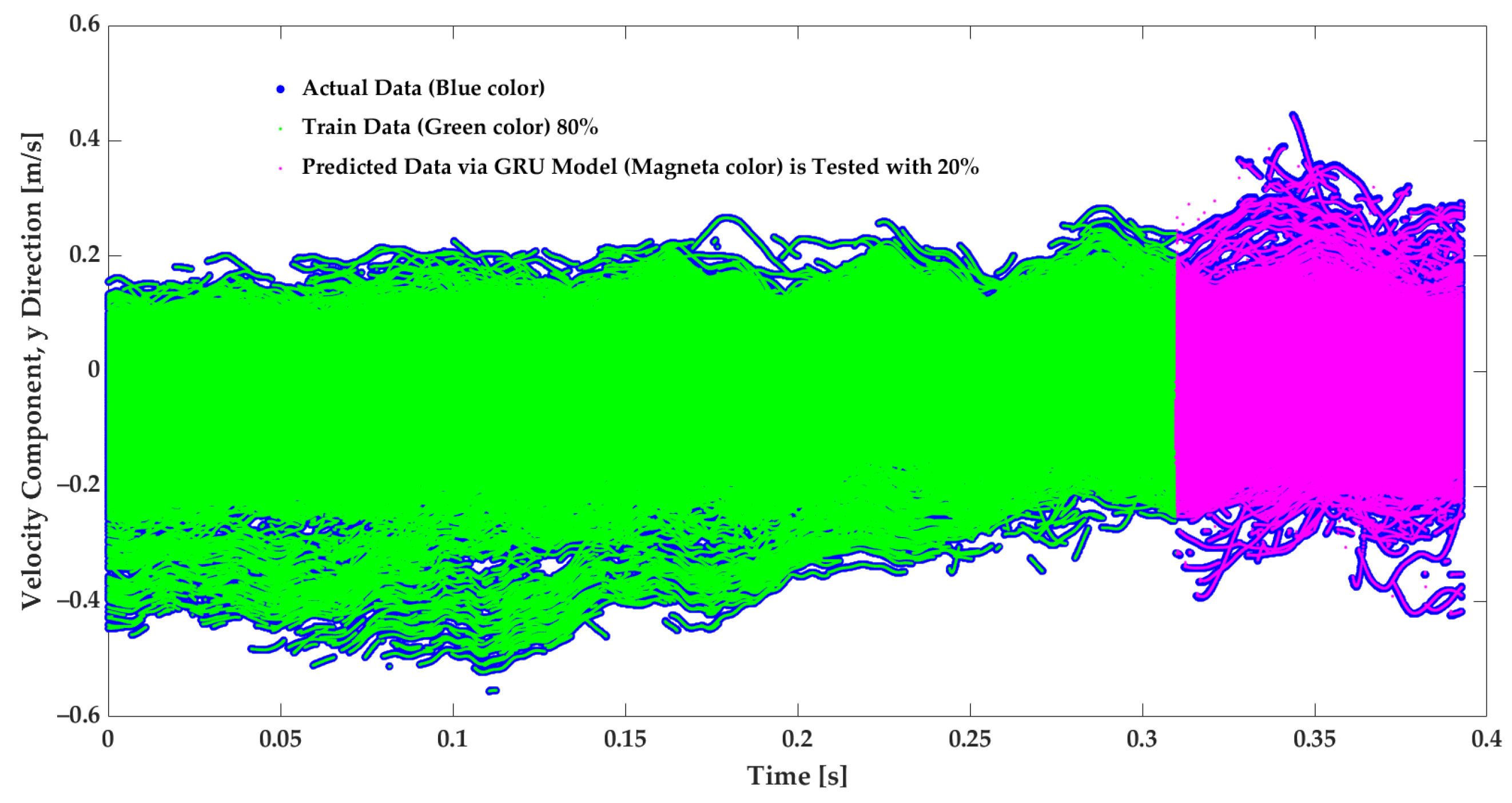
Figure 6.
Velocity prediction of the velocity in the Y direction from the GRU model. The model is trained on of the data, while the remaining is used for testing. The filled blue circles are actual data, the green points are trained data, and the magenta points are GRU-predicted data.
The model provides considerably accurate velocity forecasting. The MAE and the score metrics are applied to evaluate the model; with training data, the MAE and scores are and , respectively. It must be noted that the actual data in Figure 5 and Figure 6 are in the filled blue circles and are because of the high level of the predictions covered by the prediction.To evaluate the designed GRU model, its performance is compared to model applications from previous studies that used LSTM, GRU, and Transformer models trained only with temporal features. The comparison is displayed in Table 1. In the present study, the dataset included 6,225,457 tracking points and four sequential variables composed of x, y, and to predict the and in the following periods. The model of this work is tuned for performance in terms of the runtime and accuracy with HPO, evaluating different batch sizes, . The accuracy of the model, trained with the optimal batch size found, is specified by GRU-h in Table 1. From the previous study of the author’s research group, LSTM, GRU, and Transformer models have been applied with 2,862,119 tracking points, with two sequential variable inputs (temporal feature) composed of and to predict the and [15,16]. Table 1 shows that the GRU-h model of this study is faster than the GRU model with a smaller dataset, and it is and faster than the LSTM and Transformer models, respectively. Since the dataset in this study is approximately larger, with twice the size of input features, the modification and hyperparameter tuning made it faster, around 14–20%, which is a remarkable speed up for extensive data that could be employed in this model. Moreover, the GRU-h led to slightly more accurate predictions with an equal to 0.99 and an MAE of 0.001; see Table 1.

Table 1.
Comparison table of the GRU-h model of the current study that is improved by HPO and trained with larger data and four sequential variable inputs: x, y, , and . Transformer, LSTM, and GRU, illustrated in the table, are models from previous studies [15,16], with smaller boundary conditions and two sequential variable inputs and and without HPO.
3.3. Parallel Computing Assessment
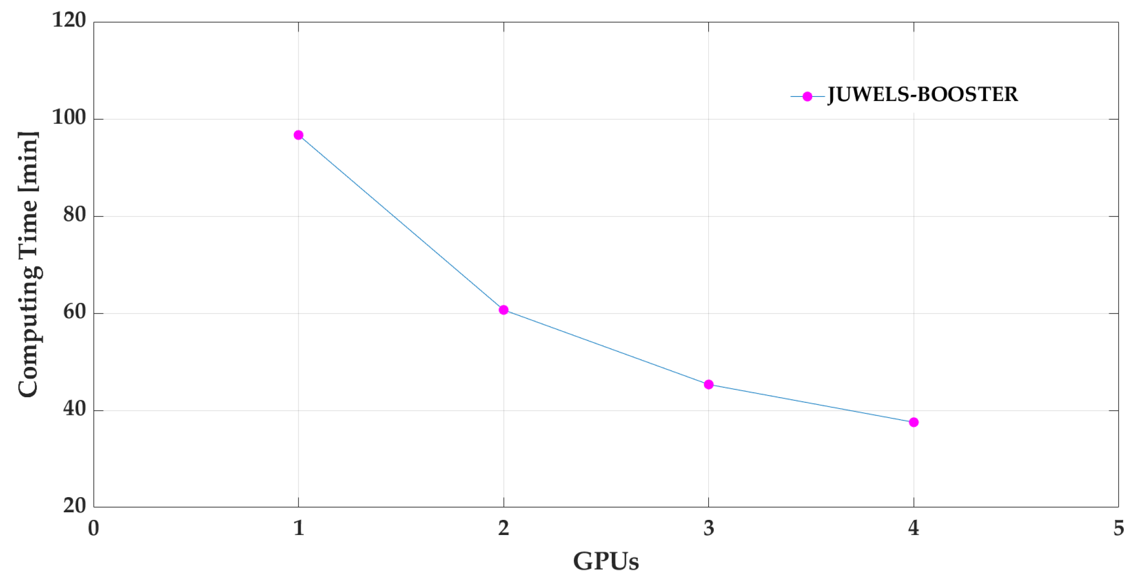
It is reported that GRU is faster and produces similar prediction results as LSTM with fewer data [4,11,12,15]. In this study, 6,225,457 tracking points are available just from the s long period of the experiment. To cope with the amount of data, the GRU is trained on parallel computing architectures, and its speed-up is examined. The training of the GRU is performed on two machines, i.e., on the DEEP-DAM and JUWELS-BOOSTER machines. On DEEP-DAM, the training is performed on a single node using one GPU. The corresponding training time using this setup is 5802.60 s, serving as a baseline. By varying the number of GPU on the JUWELS-BOOSTER, it is possible to measure the speed-up gained by the additional GPU. Here, strong scaling is the metric of choice, as the amount of work stays constant no matter how many processors are used [35]. The goal of parallelizing the computation is to reduce the time to solution. As is obvious from the data in Table 2 and Figure 7, the speed-up of the model increased with , , and for using 2, 3, and 4 GPU, respectively.
Table 2.
Parallel computing machine scalability to train the GRU model with GPU.
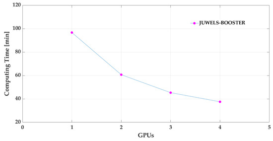
Figure 7.
Computing time on the JUWELS-BOOSTER on one node assessed with one to four GPU for the GRU training model.
In addition to the MAE, the HPO process for optimizing the batch size also affects the runtime of the training, which is reported in Table 3. As the batch size per GPU increases with a factor of 2, the total training runtime reduces approximately with the same factor. This indicates that the GPU are not fully utilized with small batch sizes, and for the computational efficiency, the training should be conducted with larger batch sizes. The lowest MAE is observed for a batch size of 512, which is an indication that this batch size is the optimal trade-off between speed-up and accuracy.
Table 3.
Effect of the size of the batch size on the computing time and the MAE.
4. Summary and Conclusions
This study employed empirical data from strained turbulence flow experiments conducted in a laboratory setup to create a velocity prediction model. The simulated turbulent flow has a Taylor microscale Reynolds number in the range of 100 < < 152. The turbulent flow at the measurement area was a nearly stationary homogeneous isotropic before the deformation. Tracer particles with a median diameter of 8–10 and a specific gravity of 1.1 were seeded in the flow. The mean strain rate in the Y direction is generated to be 4 , and the LPT technique is applied to record the flow features. Based on the Lagrangian perspective, the extracted velocity and location dataset has been used to train a GRU model for flow predictions. The strained turbulent flow is a type of shear flow that can be observed in many applications, such as the external flow over an airfoil and internal flow within a variable cross-section pipe, internal combustion in engines, particle interactions in mixing chambers, erosion at the leading edges, dispersion of pollutants in the atmosphere, formation of rain within clouds, and dispersion of sediments in oceans and rivers [17].
A GRU network is a version of the LSTM network that can perform training faster and with fewer data. As has been noted in the literature, the turbulence intensity, boundary geometry, and strain rate affect the flow velocity. Moreover, this experiment was performed in the presence of gravity, which was not investigated in previous numerical studies on deformed turbulent flow, and its effect remains unknown. This study relies on the concept that the velocity as a function of the locations and sequential feature of the flow carries all relevant information affecting the above-mentioned factors. Therefore, in the training of the GRU, the model is evaluated to observe how it is capable of learning how the historical effect of all parameters will impact the following period, since DL can extract hidden features. Each velocity component and location are measured by LPT in sequence form, and the locations x, y, and velocity components in the corresponding directions are applied as input data to train the GRU model. Based on the training, the GRU predicts the velocity component individually in the following period. In this study, of the data was used as training data, and the remaining of the data were employed to test the prediction and validate it.
The predictions from the GRU model are considerably accurate, as the MAE and score are 0.001 and 0.993, respectively. The suggested approach leads to predicting turbulence flow in many applications. However, it is essential to evaluate the model with extensive data and long-term predictions, as well as apply different boundary conditions and vary the Reynolds number range to observe the limit of the projections. The current model has been compared to previous DL models with a similar application. The results in Table 1 show that the proposed model, with larger data and two times more input variables, has a faster performance of 14–20% than similar model applications of LSTM, GRU, and Transformer because of the HPO. This performance is a remarkable achievement, particularly when applying the model to a more extensive dataset. Besides the accurate predictions generated by this model, the model was executed on the parallel machines JULES-BOOSTER and DEEP-DAM at the Jülich Supercomputer Centre to investigate the training’s speed-up. The performance on one node and one to four GPU has been examined in JUWELS-BOOSTER. The results show the speed-up to increase in two GPU. With four GPU, the model trains faster than the metric measurement with a single GPU. To further enhance this model, its performance with respect to the prediction accuracy and scalability will be examined extensively using more data. Furthermore, the impact of the hyperparameters in this model will be investigated to accelerate the model under the constraint of keeping the accuracy at suitable conditions.
Author Contributions
R.H. contributed to the conceptualization, method, software, data analysis, and writing—original draft preparation. M.A. contributed to the software, methodology, and model analysis. A.L. contributed to the review and editing. Á.H. contributed to the review and editing. M.R. contributed to the writing, review editing, and supervision. All authors have read and agreed to the published version of the manuscript.
Funding
The research leading to these results has been conducted in the Center of Excellence (CoE) Research on AI and Simulation-Based Engineering at Exascale (RAISE), the EuroCC two projects receiving funding from EU’s Horizon 2020 Research and Innovation Framework Programme, and European Digital Innovation Hub Iceland (EDIH-IS) under the grant agreement no. 951733, no. 101101903, and no. 101083762, respectively.
Institutional Review Board Statement
Not applicable.
Informed Consent Statement
Not applicable.
Data Availability Statement
The data presented in this study are available on request from the corresponding author.
Acknowledgments
We thank Ármann Gylfason from Reykjavik University for his technical comments on the experimental data and Lahcen Bouhlali from Reykjavik University for his experimental work in data preparation. The authors thank the technical support of the FreaEnergy team (Energy, AI, HPC, and CFD solutions), at Mýrin located in the Gróska -innovation and business growth center- in Reykjavik.
Conflicts of Interest
The authors declare no conflicts of interest.
Abbreviations
| CFD | Computational Fluid Dynamics |
| CNN | Convolutional Neural Network |
| CPU | Central Processing Unit |
| DL | Deep Learning |
| DMD | Dynamical Mode Decomposition |
| DNS | Direct Numerical Simulation |
| GPU | Graphics Processing Unit |
| GRU | Gated Recurrent Unit |
| HPC | High-Performance Computing |
| HPO | Hyperparameter Optimization |
| LES | Large Eddy Simulation |
| LPT | Lagrangian Particle Tracking |
| LSTM | Long Short-Term Memory |
| MAE | Mean Absolute Error |
| ML | Machine Learning |
| MLP | Multilayer Perceptron |
| MPI | Message Passing Interface |
| POD | Proper Orthogonal Decomposition |
| RANS | Reynolds-Averaged Navier Stokes |
| RANS | Reynolds-Averaged Navier Stokes |
| RNN | Recurrent Neural Network |
| ROM | Reduced-Order Model |
References
- Pope, S.B. Turbulent Flows; Cambridge University Press: London, UK, 2000. [Google Scholar]
- John, L.; Lumley, H.T. A First Course in Turbulence; MIT Press: Cambridge, MA, USA, 1972. [Google Scholar]
- Davidson, P.A. Turbulence: An Introduction for Scientists and Engineers; Oxford University Press: London, UK, 2004. [Google Scholar]
- Hassanian, R.; Riedel, M.; Bouhlali, L. The Capability of Recurrent Neural Networks to Predict Turbulence Flow via Spatiotemporal Features. In Proceedings of the 2022 IEEE 10th Jubilee International Conference on Computational Cybernetics and Cyber-Medical Systems (ICCC), Reykjavík, Iceland, 6–9 July 2022; pp. 000335–000338. [Google Scholar] [CrossRef]
- Bukka, S.R.; Gupta, R.; Magee, A.R.; Jaiman, R.K. Assessment of unsteady flow predictions using hybrid deep learning based reduced-order models. Phys. Fluids 2021, 33, 013601. [Google Scholar] [CrossRef]
- Cengel, Y.; Cimbala, J. Fluid Mechanics Fundamentals and Applications; McGraw Hill: New York, NY, USA, 2013. [Google Scholar]
- White, F. Fluid Mechanics; McGraw Hill: New York, NY, USA, 2015. [Google Scholar]
- Eivazi, H.; Veisi, H.; Naderi, M.H.; Esfahanian, V. Deep neural networks for nonlinear model order reduction of unsteady flows. Phys. Fluids 2020, 32, 105104. [Google Scholar] [CrossRef]
- Srinivasan, P.A.; Guastoni, L.; Azizpour, H.; Schlatter, P.; Vinuesa, R. Predictions of turbulent shear flows using deep neural networks. Phys. Rev. Fluids 2019, 4, 054603. [Google Scholar] [CrossRef]
- Hochreiter, S.; Schmidhuber, J. Long Short-Term Memory. Neural Comput. 1997, 9, 1735–1780. [Google Scholar] [CrossRef] [PubMed]
- Wang, Y.; Zou, R.; Liu, F.; Zhang, L.; Liu, Q. A review of wind speed and wind power forecasting with deep neural networks. Appl. Energy 2021, 304, 117766. [Google Scholar] [CrossRef]
- Gu, C.; Li, H. Review on Deep Learning Research and Applications in Wind and Wave Energy. Energies 2022, 15, 1510. [Google Scholar] [CrossRef]
- Duru, C.; Alemdar, H.; Baran, O.U. A deep learning approach for the transonic flow field predictions around airfoils. Comput. Fluids 2022, 236, 105312. [Google Scholar] [CrossRef]
- Moehlis, J.; Faisst, H.; Eckhardt, B. A low-dimensional model for turbulent shear flows. New J. Phys. 2004, 6, 56. [Google Scholar] [CrossRef]
- Hassanian, R.; Helgadottir, A.; Riedel, M. Deep Learning Forecasts a Strained Turbulent Flow Velocity Field in Temporal Lagrangian Framework: Comparison of LSTM and GRU. Fluids 2022, 7, 344. [Google Scholar] [CrossRef]
- Hassanian, R.; Myneni, H.; Helgadottir, A.; Riedel, M. Deciphering the dynamics of distorted turbulent flows: Lagrangian particle tracking and chaos prediction through transformer-based deep learning models. Phys. Fluids 2023, 35, 075118. [Google Scholar] [CrossRef]
- Hassanian, R.; Helgadottir, A.; Bouhlali, L.; Riedel, M. An experiment generates a specified mean strained rate turbulent flow: Dynamics of particles. Phys. Fluids 2023, 35, 015124. [Google Scholar] [CrossRef]
- Pant, P.; Doshi, R.; Bahl, P.; Barati Farimani, A. Deep learning for reduced order modelling and efficient temporal evolution of fluid simulations. Phys. Fluids 2021, 33, 107101. [Google Scholar] [CrossRef]
- Fresca, S.; Manzoni, A. POD-DL-ROM: Enhancing deep learning-based reduced order models for nonlinear parametrized PDEs by proper orthogonal decomposition. Comput. Methods Appl. Mech. Eng. 2022, 388, 114181. [Google Scholar] [CrossRef]
- Papapicco, D.; Demo, N.; Girfoglio, M.; Stabile, G.; Rozza, G. The Neural Network shifted-proper orthogonal decomposition: A machine learning approach for non-linear reduction of hyperbolic equations. Comput. Methods Appl. Mech. Eng. 2022, 392, 114687. [Google Scholar] [CrossRef]
- Riedel, M.; Sedona, R.; Barakat, C.; Einarsson, P.; Hassanian, R.; Cavallaro, G.; Book, M.; Neukirchen, H.; Lintermann, A. Practice and Experience in using Parallel and Scalable Machine Learning with Heterogenous Modular Supercomputing Architectures. In Proceedings of the 2021 IEEE International Parallel and Distributed Processing Symposium Workshops (IPDPSW), Portland, OR, USA, 17–21 June 2021; pp. 76–85. [Google Scholar] [CrossRef]
- Hassanian, R.; Riedel, M. Leading-Edge Erosion and Floating Particles: Stagnation Point Simulation in Particle-Laden Turbulent Flow via Lagrangian Particle Tracking. Machines 2023, 11, 566. [Google Scholar] [CrossRef]
- Cowen, E.A.; Monismith, S.G. A hybrid digital particle tracking velocimetry technique. Exp. Fluids 1997, 22, 199–211. [Google Scholar] [CrossRef]
- Hassanian, R. An Experimental Study of Inertial Particles in Deforming Turbulence Flow, in Context to Loitering of Blades in Wind Turbines. Master’s Thesis, Reykjavik University, Reykjavik, Iceland, 2020. [Google Scholar]
- Ouellette, N.T.; Xu, H.; Bodenschatz, E. A quantitative study of three-dimensional Lagrangian particle tracking algorithms. Exp. Fluids 2006, 40, 301–313. [Google Scholar] [CrossRef]
- Lee, C.M.; Gylfason, A.; Perlekar, P.; Toschi, F. Inertial particle acceleration in strained turbulence. J. Fluid Mech. 2015, 785, 31–53. [Google Scholar] [CrossRef]
- Ayyalasomayajula, S.; Warhaft, Z. Nonlinear interactions in strained axisymmetric high-Reynolds-number turbulence. J. Fluid Mech. 2006, 566, 273–307. [Google Scholar] [CrossRef]
- Cho, K.; van Merriënboer, B.; Bahdanau, D.; Bengio, Y. On the Properties of Neural Machine Translation: Encoder–Decoder Approaches. arXiv 2014, arXiv:1409.1259. [Google Scholar]
- Chung, J.; Gulcehre, C.; Cho, K.; Bengio, Y. Empirical evaluation of gated recurrent neural networks on sequence modeling. arXiv 2014, arXiv:1412.3555. [Google Scholar]
- Abadi, M.; Agarwal, A.; Barham, P.; Brevdo, E.; Chen, Z.; Citro, C.; Corrado, G.S.; Davis, A.; Dean, J.; Devin, M.; et al. Tensorflow: Large-scale machine learning on heterogeneous distributed systems. arXiv 2016, arXiv:1603.04467. [Google Scholar]
- Abadi, M.; Barham, P.; Chen, J.; Chen, Z.; Davis, A.; Dean, J.; Devin, M.; Ghemawat, S.; Irving, G.; Isard, M.; et al. Tensorflow: A system for large-scale machine learning. In 12th USENIX Symposium on Operating Systems Design and Implementation; USENIX Association: Berkeley, CA, USA, 2016. [Google Scholar]
- Kramer, O. Scikit-learn. Mach. Learn. Evol. Strateg. 2016, 20, 45–53. [Google Scholar]
- Alvarez, D. JUWELS Cluster and Booster: Exascale Pathfinder with Modular Supercomputing Architecture at Juelich Supercomputing Centre. J. Large-Scale Res. Facil. JLSRF 2021, 7, A183. [Google Scholar] [CrossRef]
- TensorFlow. TensorFlow Core Tutorials; TensorFlow: Mountain View, CA, USA, 2022. [Google Scholar]
- Hager, G.; Wellein, G. Introduction to High Performance Computing for Scientists and Engineers; Chapman & Hall/CRC Computational Science: London, UK, 2010. [Google Scholar]
Disclaimer/Publisher’s Note: The statements, opinions and data contained in all publications are solely those of the individual author(s) and contributor(s) and not of MDPI and/or the editor(s). MDPI and/or the editor(s) disclaim responsibility for any injury to people or property resulting from any ideas, methods, instructions or products referred to in the content. |
© 2024 by the authors. Licensee MDPI, Basel, Switzerland. This article is an open access article distributed under the terms and conditions of the Creative Commons Attribution (CC BY) license (https://creativecommons.org/licenses/by/4.0/).