Abstract
Pipe structures are commonly encountered in the geophysical context, and in particular in sedimentary basins, where they are associated with fluid migration structures. We investigate pipe formation through laboratory experiments by injecting water locally at a constant flow rate at the base of water-saturated sands in a Hele–Shaw cell (30 cm high, 35 cm wide, gap 2.3 mm). The originality of this work is to quantify the effect of a discontinuity. More precisely, bilayered structures are considered, where a layer of fine grains overlaps a layer of coarser grains. Different invasion structures are reported, with fluidization of the bilayered sediment over its whole height or over the finer grains only. The height and area of the region affected by the fluidization display a non-monotonous evolution, which can be interpreted in terms of fluid focusing vs. scattering. Theoretical considerations can predict the critical coarse grains height for the invasion pattern transition, as well as the maximum topography at the sediment free surface in the regime in which only the overlapping finer grains fluidize. These results have crucial geophysical implications, as they demonstrate that invasion patterns and pipe formation dynamics may control the fluid expulsion extent and localization at the seafloor.
1. Introduction
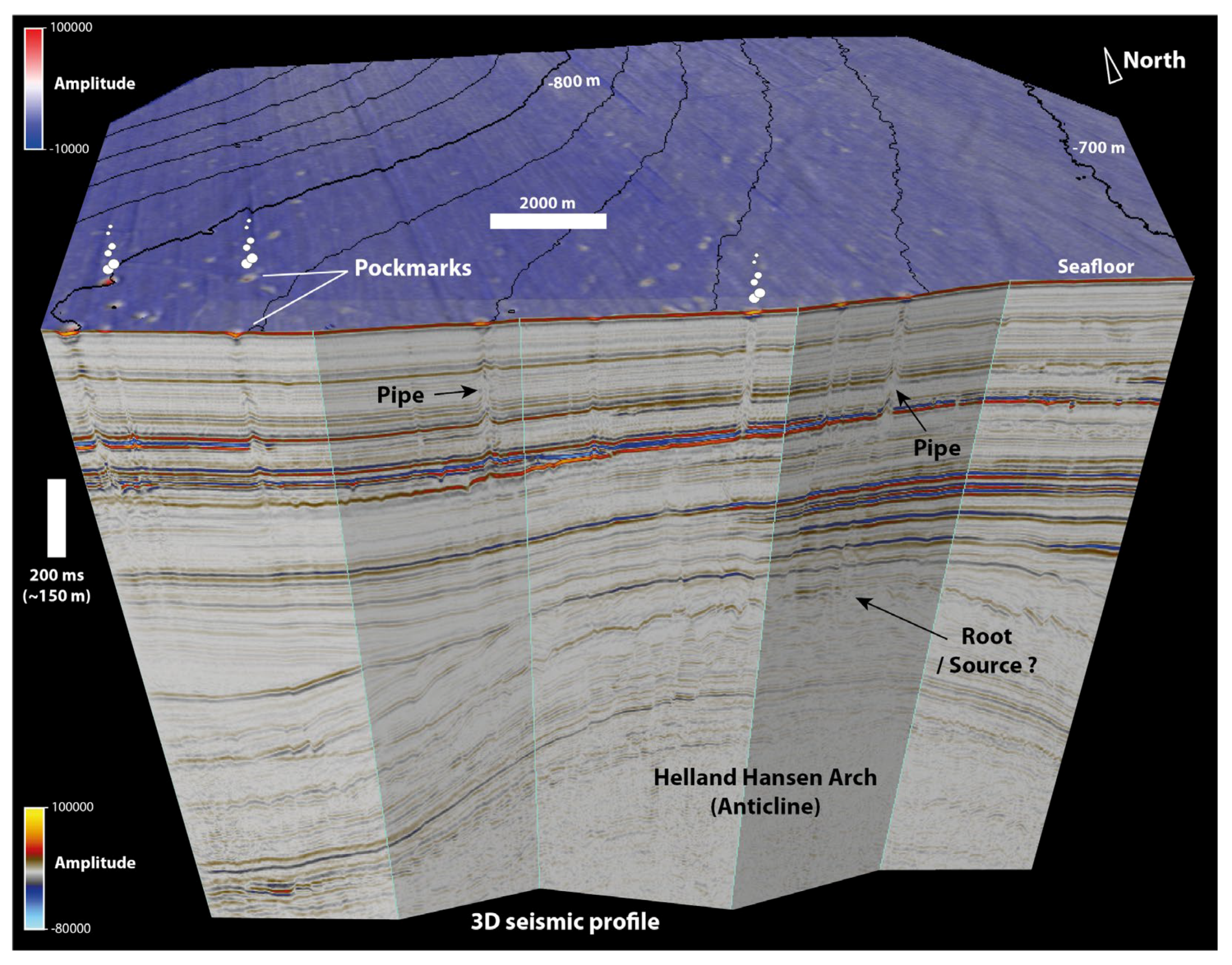
In the geophysical context, “pipes” refer to structures of upward fluid migration in sedimentary basins, followed by fluid expulsion at the seafloor [1,2,3,4]. They are easily recognizable in seismic profiles, where reflectors corresponding to the different sedimentary layers are locally disturbed by the fluid rise and exhibit a vertical chimney (Figure 1). On the seafloor, these structures display a topography anomaly ranging from tens of meters up to a few kilometers [5]. In recent decades, they have increasingly focused the attention of the geophysical community due to their risk potential. On the one hand, fluid expulsion at the seafloor may trigger slope instability and large submarine landslides; on the other hand, they represent strong geohazards for anthropic activities such as offshore resources, transoceanic telecom fibers and CO2 sequestration. Lastly, massive greenhouse fluid emissions have been correlated to important climate changes in Earth’s history [6,7,8,9,10,11].
Although pipes in sedimentary basins have been extensively characterized (see, among many other examples, [2,5,12,13,14]) and new technologies provide more and more extensive and high-quality geophysical data, images and measurements at the seafloor only provide a present-day picture of these processes. The challenge, therefore, is to obtain insights into their dynamics—either short or long term—to evaluate their risk potential [15]. To do so, many analogue experiments [16,17,18,19,20,21,22,23,24,25] and numerical models [4,13,22,25,26,27,28] have been proposed in the literature (see also [29] for a complementary review). However, these models mostly consider a homogeneous sedimentary bed and scarcely account for its complex structure. Sedimentary basins are characterized by successive deposits, which appear as multiple reflectors in the seismic profiles, making it look like a geological millefeuille, with multiple layers exhibiting different physical properties (Figure 1). To our knowledge, few studies in the literature consider the effect of discontinuities, i.e., interfaces between two layers of different properties, on sediment mobilization and fluid escape structures [16,19,30]. The few existing works mainly focus on the effect of cohesion of the covering layer. Therefore, there is a gap in the literature about fundamental studies of the effect of a discontinuity between two layers of different granulometry on upward fluid migration and pipe formation.

Figure 1.
A 3D view of a fluid expulsion province in the Norway Basin (Helland Hansen Arch) [31]. Deep and shallow fluids migrate through a millefeuille of layers with different physical properties (porosity, permeability, cohesion, etc.) leading to focused fluid migration (pipes) and expulsion (pockmarks). These structures are identified on geophysical records as high-amplitude anomalies and/or dimming of reflectors. Even with the best resolution available, the root (or source) of fluids remains debated.
The present work aims at quantifying pipe formation and evolution in a bilayered sediment, considering non-cohesive granular materials. The goal here is to provide a precise quantification of the pipe dynamics in a non-cohesive sediment, in the presence of a discontinuity, to investigate its effect on the fluid focalization. To do so, we will consider a bilayer made of large grains at the bottom, and small grains overlaying the large grains. “Large grains” here refer to grains large enough so that without the smaller grains on their top, the fluid percolates through them—except for very thin monolayers. Conversely, a monolayer of “small grains” always displays fluidization in the range of parameters explored in this work. In the following, we present the materials and methods (Section 2). We then describe the formation of pipes, i.e., focalized fluid migration, in bilayered sediments, when varying the total sediment height or the ratio between the large and small grains height (Section 3). The results are finally discussed in Section 4.
2. Materials and Methods
2.1. Experimental Setup
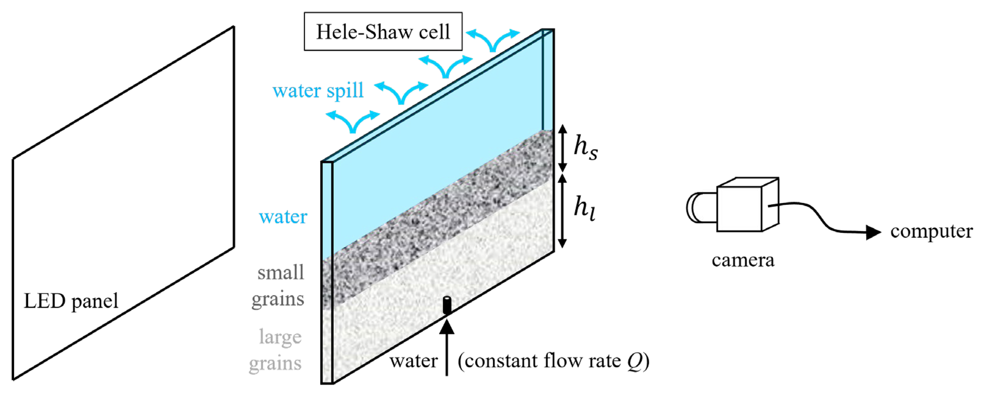
The experimental setup (Figure 2) consists of a Hele–Shaw cell made of two glass plates (height 30 cm, width cm) separated by a thin gap ( mm). This configuration makes it possible to visualize the migration pattern of the incoming fluid, which is otherwise impossible to see in opaque granular media. The cell is filled with a granular bed (see Section 2.2), initially immersed in clear distilled water (density kg.m−3). At the beginning of the experiment, water at a constant flow rate is injected locally at the bottom center of the cell via a cylindrical nozzle (inner diameter 1.1 mm). The injected water is dyed in dark blue (food dye Meilleur du Chef E133, 0.6% vv.) so that it can be distinguished from the water in which the grains are initially deposited. It has been checked that the dye does not modify the physical properties of the liquid. The flow rate is imposed using a pump (Tuthill 7.11.468) coupled with a flow controller (Bronkhorst mini CORI-FLOW M14-AAD-22-0-S) and can be varied in the range of 2–100 mL/min. The water exits the system uniformly by the top cell aperture by overflow (Figure 2) and is collected using a gully surrounding the cell’s top part.
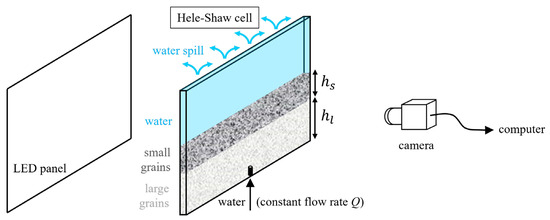
Figure 2.
Experimental setup. The water spill system (by overflow) and the flow controller devices are not shown.
The cell is illuminated by transmission with a homogeneous light panel (Just Normlicht Classic Line) located behind the cell. Images are recorded with a camera (Basler monochrome, acA2040-90 μm, 2048 × 2048 pixels) mounted with a 16 mm or 25 mm lens, depending on the experiments. A calibration grid is used prior to each experiment to provide a precise conversion from pixels to mm. The acquisition frequency is set between 10 and 36 fps depending on the experiment. All experiments are performed at room temperature.
2.2. Granular Media
The grains used in the experiments are polydisperse spherical glass beads with a density kg.m−3. Polydispersity is chosen on purpose; first, to avoid crystallization, a process that classically occurs in monodisperse spherical beads; and second, to mimick the polydispersity of natural sands. Two batches have been used to compose the bilayered sediment. The bottom layer (height , Figure 2) is made of the larger grains (USF Matrasur, diameter 425–600 μm). The smaller grains (Wheelabrator, diameter 106–212 μm) are located in the top layer (height , Figure 2), covering the sediments of a larger size. In the following, we will refer to these two batches as the “large grains” and “small grains”, respectively. In the following, the total initial sediment height is .
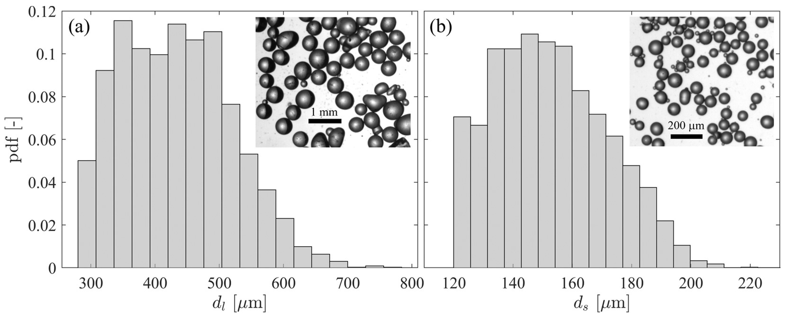
The particle size distribution has been measured with a macroscope (Wild Makroscop M420 1.25×) mounted with a Makrozoom Leica 1:5 lens. Figure 3 displays the particle size distribution for the two grain batches.
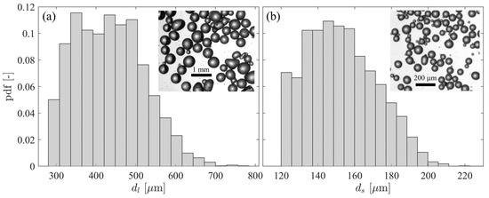
Figure 3.
Particle size distribution (power density function) (a) for the large grains ( 425–600 μm, over 3653 particles) and (b) the small grains ( 106–212 μm, over 3333 particles).
3. Results
3.1. Invasion Regimes
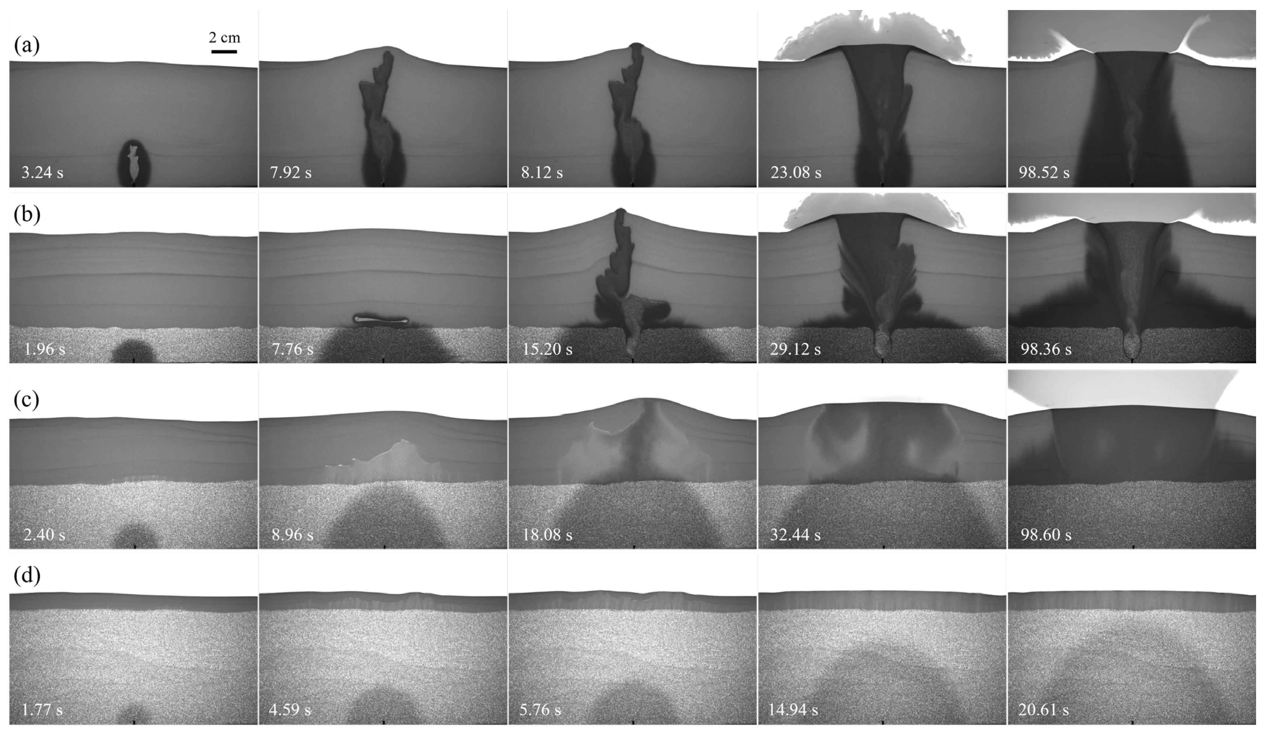
Figure 4 displays the different invasion regimes for a constant total granular layer height (here, 11 cm) when varying the ratio between the large and small grains, . As stated in the introduction, the “small grains” are chosen so that, in our experimental range, a monolayer of such grains always fluidizes (Figure 4a, Supplemental Video S1). The fluid penetrates the granular layer, forming a finger, which propagates upwards until reaching the granular free surface. At long times (Figure 4a, t = 98.52 s), the central fluidized zone has a specific shape well known in the geophysical context as the “stem and corolla” shape, with a vertical chimney topped by a flared area, also referred to as a “funnel and pipe” structure [5,32]. Note that the granular layer fluidization is coupled with percolation around the central zone since the initial invasion (Figure 4a, t = 3.24 s), and the lateral invasion due to this process increases in time (Figure 4a, t = 98.52 s).
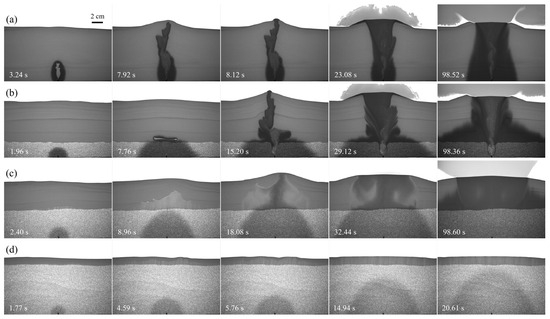
Figure 4.
Different invasion regimes for a constant height when varying the large-to-small grain ratio [ mL/min]. (a) Monolayer of small grains [ cm, Video S1]. (b) Fluidization of both layers of grains [ cm, cm, Video S2]. (c) Percolation in the bottom layer, fluidization of the small grains [ cm, cm, Video S3]. (d) Percolation in the bottom layer, fluidization of the small grains [ cm, cm, Video S4].
Conversely, the “large grains” are chosen so that a monolayer of such grains, when high enough ( cm), is in the percolation regime, i.e., the invading fluid will propagate through the pore network without moving the grains significantly. For very thin layers ( cm), a “large-grain” monolayer exhibits fluidization. When introducing a small large-grain layer at the bottom of the experiment (Figure 4b, Supplemental Video S2), independently of the monolayer behavior, a percolation invasion regime always occurs at the first instant (Figure 4b, t = 1.96 s). However, when the invading fluid reaches the interface, it generates a horizontal decompaction zone (Figure 4b, t = 7.76 s, light region above the interface). This decompaction zone fluidizes the upper small-grain layer by generating, as in the above monolayer configuration, a finger that propagates upwards. In addition, it is capable of fluidizing the large grains layer, too, by entraining the particles above the injection nozzle.
An interesting change in the invasion regime appears when the ratio reaches a critical value. Above this value, the flow-scattering due to the percolation process is strong enough that the effective flux crossing the interface is not able to entrain the large particles anymore, even at long times (Figure 4c,d, Supplemental Videos S3 and S4). Note that for our experimental parameters, the above small-grain layer is always fluidized. It is interesting to note that due to the fluid’s incompressibility, the decompaction and fluidization above the interface starts before the dyed injected fluid reaches the interface (see, for instance, Figure 4c, t = 2.40 s). It therefore acts as a secondary source, located at the interface, with a spatial extent given by the properties of the medium.
Figure 5 summarizes the different invasion patterns when varying the total height of the sediments and the ratio between the large and small grains. The experimental points for a large or small-grain monolayer are reported in black with, as expected, percolation (black squares) or fluidization (black triangles), respectively. In the bilayer, the region where both layers fluidize (gray region, gray diamonds) can be clearly distinguished from the region where the invading fluid always percolates in the bottom (large-grain) layer, while it fluidizes the above (small-grain) layer (white region, white dots). Interestingly, the transition does not depend on and seems controlled by a critical large-grain height, cm. This constant value will be discussed in Section 4.1. Note that for this critical value, an intriguing behavior arises. Indeed, a monolayer of large grains with exhibits percolation. When adding a small-grain layer on top, the large grains still exhibit a percolation regime (white dots, Figure 5) until a critical load. When reaching cm, the system exhibits fluidization in both layers. The reproducibility of such behavior has been checked by repeating the experiments (double symbols, Figure 5).
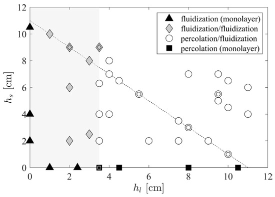
Figure 5.
Regime diagram for the invasion patterns [ mL/min]. For a monolayer, the system always fluidizes (small grains, black triangles) or percolates (large grains, black squares). Note that a large-grain monolayer may exhibit fluidization for a small height ( cm). For a bilayer, we report either fluidization of both layers (gray region, gray diamonds) or percolation in the large grains topped by fluidization of the above small grains layer (white region, white dots). The dashed line represents a constant total height cm, corresponding to the series of experiments most studied in this work. Double symbols indicate reproducibility check.
Next, in Section 3.2, we investigate the pipe formation dynamics. Unless otherwise stated, we will present results associated with a constant total sediment height, when varying the ratio (Figure 5, dashed line).
3.2. Pipe Formation Dynamics
3.2.1. Decompaction Front
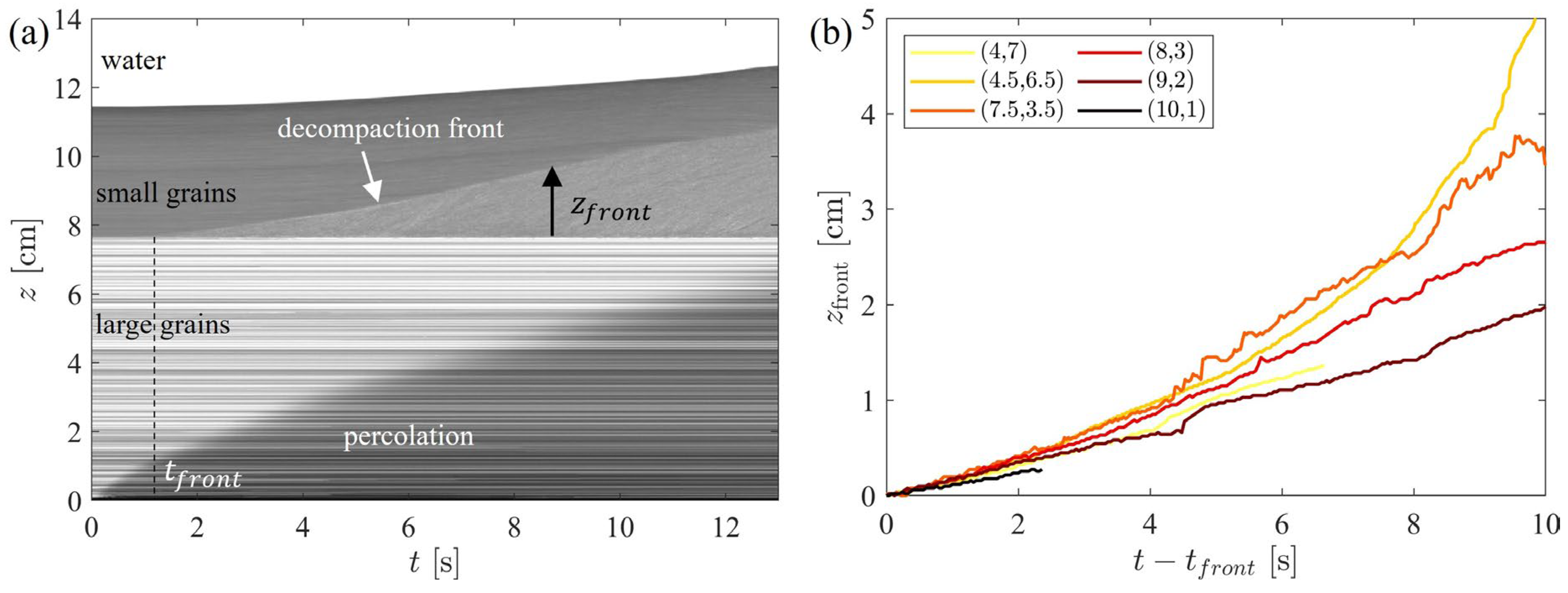
As reported above, the pipe always initiates at the interface. Figure 6a displays a spatiotemporal diagram showing the dynamics of pipe initiation and formation. This diagram reports, for each time t, the intensity along a vertical line above the injection nozzle. This line, at , is characterized by the signature of the large-grain layer (white and dark pattern from to 8 cm) and the small-grain layer (darker gray from to 11 cm), topped with clear water (Figure 6a). Note here that although spatiotemporal diagrams are convenient to characterize the pipe dynamics, they have to be considered with caution. In particular, they can be interpreted only during the first stage of the pipe formation. Indeed, the pipe can later shift offline with respect to the vertical of the nozzle (see, for instance, Figure 4b, s, left shift or Figure 4c, s, right shift). If such a shift happens, the spatiotemporal diagram is not representative anymore of the topmost fluidized point, and the pipe dynamics may thus be misinterpreted. In particular, as the topmost fluidized point displays the fastest upward velocity, interpreting the spatiotemporal diagram in such a case may lead to an underestimation of the pipe front velocity.
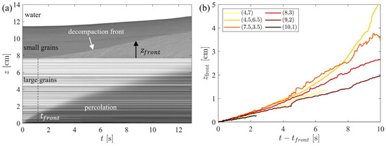
Figure 6.
Dynamics of pipe initiation and formation. (a) Spatiotemporal diagram of the intensity along a vertical line above the injection nozzle [ cm, cm, mL/min]. At time , the dyed water invades the large grains (percolation, bottom dark region). The fluidization starts at the interface at time , via a decompaction front that propagates upwards (light gray region in the small-grain layer). (b) Decompaction front elevation from the interface, , as a function of time counted from the decompaction front generation, , for different granular layers [cm] indicated in the legend. Note the linear behavior at short times.
At , the dyed water invades the large-grain layer from the bottom upwards (bottom dark region, Figure 6a). As the fluid migrates by percolation, the large grains do not move, resulting in fixed horizontal lines in the spatiotemporal diagram. After a time , a decompaction front initiates at the interface, then grows and propagates upwards (light gray region in the small grains layer, Figure 6a). Figure 6b displays the altitude of this decompaction front, , as a function of time from its initiation, . At short times, it varies linearly in time, indicating a constant initiation velocity.
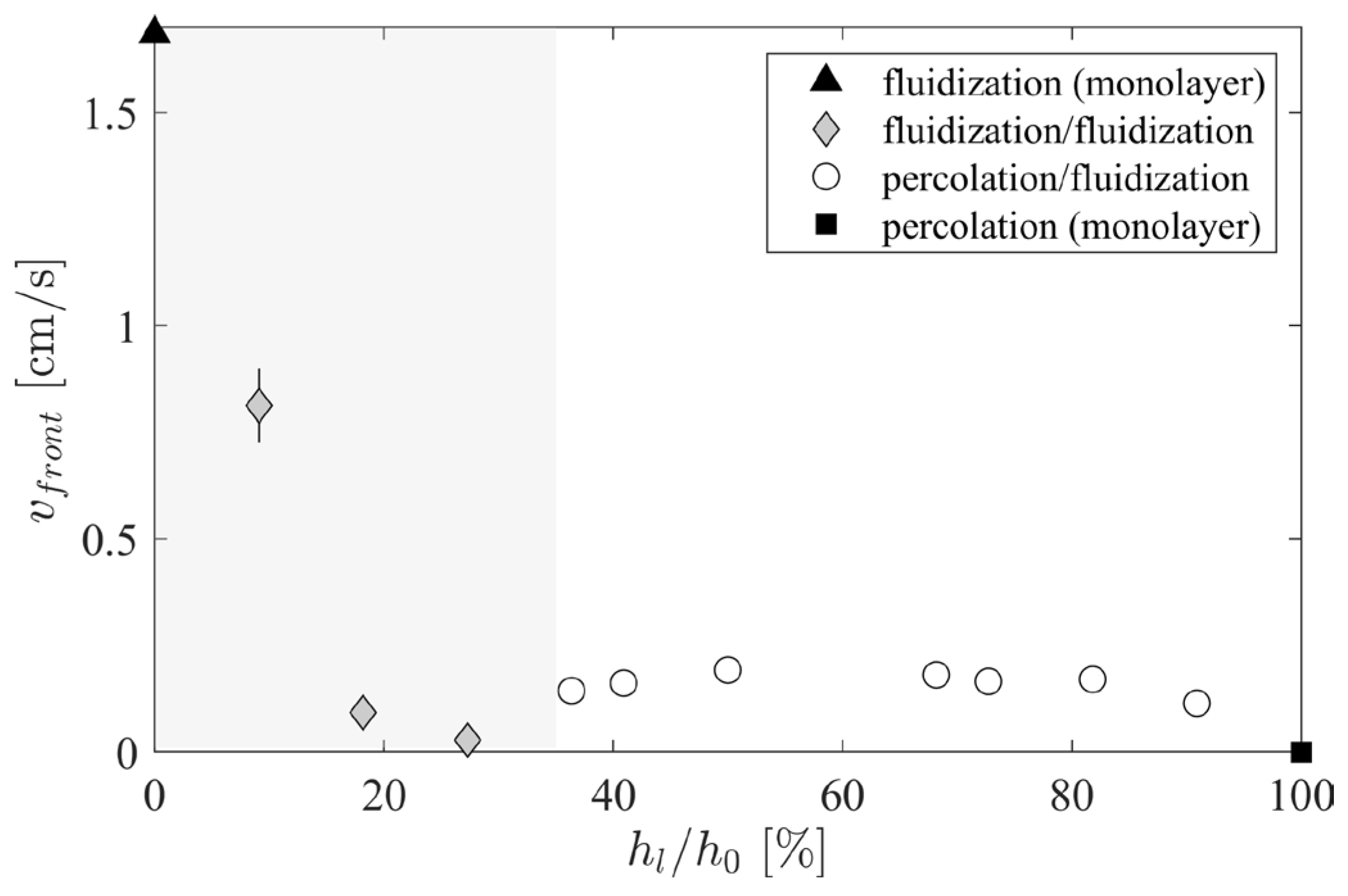
Figure 7 displays the decompaction front velocity as a function of the percentage of large grains, , for a constant initial sediment height . When introducing a small large grains layer at the bottom, the system, although exhibiting an initial percolation in the large grains layer, still fully fluidizes (gray diamonds, Figure 7), but the decompaction front velocity drops drastically—by almost two orders of magnitude for ~30% of large grains at the bottom. When increasing the large-to-small grains ratio, we enter the regime where the fluidization of the top small-grain layer is not able to entrain the large grains anymore. The bottom large-grain layer remains in the percolation regime, and the decompaction front velocity in the above layer exhibits an almost constant value (~0.1–0.2 cm/s, white dots, Figure 7).

Figure 7.
Decompaction front velocity as a function of the large grain ratio , in percents [ cm, mL/min]. If not visible, the error bars are smaller than the symbol size. The white and gray regions indicate the invasion regimes (Figure 5).
The drastic drop in the decompaction front velocity is the consequence of the large-grain layer which acts as a scatterer for the incoming fluid. Even in the fluidization/fluidization regime, the fluid first invades the large-grain layer by percolation, before reaching the interface with the small grains and decompacting/fluidizing the whole system. Compared to a direct injection via the bottom nozzle, the fluid spread by the large grains reaches the small-grain layer with a much lower velocity, resulting henceforth in a slower decompaction process and a drastic drop in the decompaction front velocity.
3.2.2. Fluidization
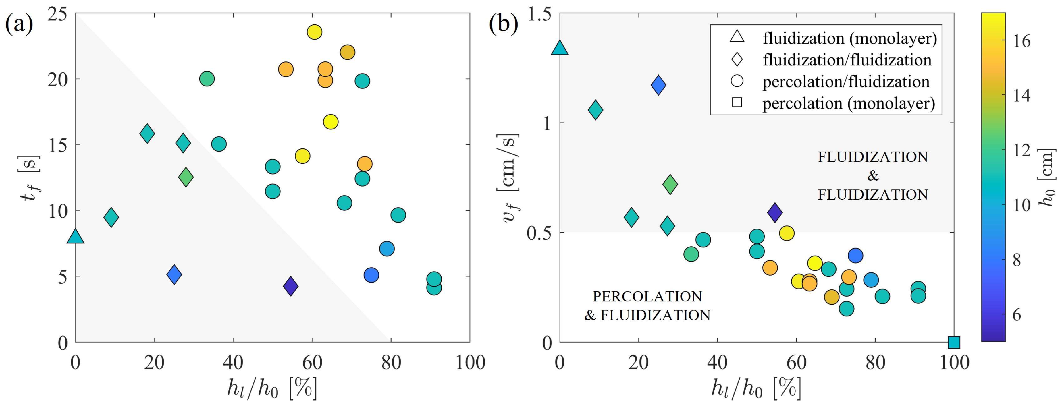
After its formation, the decompaction front propagates upwards until reaching the free surface. We define the fluidization time, , as the time between the start of injection, when the fluid first enters the system, until the time at which the fluidized region reaches the free surface of the sediment bilayer. Figure 8a displays the fluidization time as a function of the large-grain percentage, . Experimental data are reported here for different initial sediment height (colorbar, Figure 8, right). In spite of different initial conditions ( and ), the data are well organized into two distinct regions. The higher the large-grain percentage in the bilayer, the smaller the fluidization time at the transition between the two regimes (fluidization of both layers, diamonds, and fluidization of the top layer only, dots). This result may be surprising, as, when increases, one may think that the percolation will take longer to propagate up to the interface and then fluidize the smaller grains layer. However, it is important here to remember that, due to fluid incompressibility, as soon as the fluid is injected at the cell bottom, it propagates through the whole cell, including the small-grain layer, by percolation or fluidization.
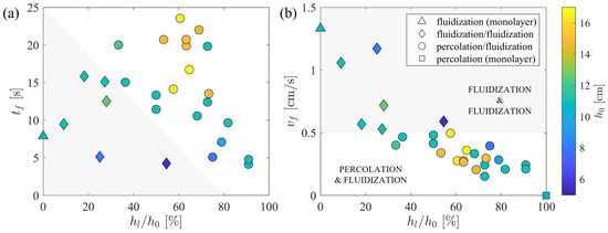
Figure 8.
(a) Fluidization time and (b) fluidization velocity as a function of the percentage of large grains, (see text). The error bars (~3 images at 36 fps corresponding to ~80 ms for ) are smaller than the symbol size. The symbols and white and gray regions indicate the invasion regimes (see Figure 5), while the colorbar (same for both figures) indicates the initial sediment height [ mL/min].
To better understand the fluidization process, we report in Figure 8b the fluidization velocity, defined as . It represents the average velocity of fluidization for the small-grain layer. Once again, all experimental data are grouped in two distinct regions, separating the two invasion regimes. This result makes it possible to define a critical fluidization velocity of about 0.5 cm/s, below which the flow is not able to entrain the large grains and fluidizes the small grains layer only. These results will be further discussed in Section 4.
3.3. Height and Area of the Granular Bed
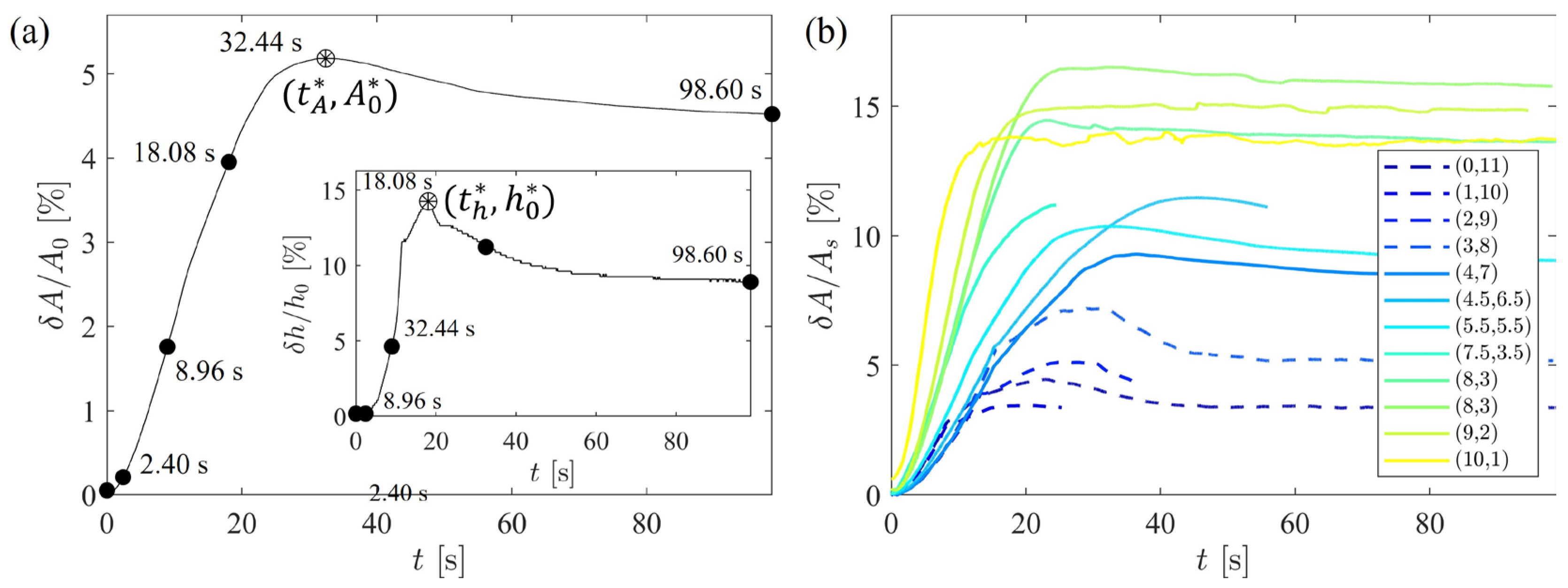
When the sediment layer starts fluidizing, due to decompaction, we observe a deformation of the free surface. The free surface topography first increases, until the fluidized region reaches the surface (Figure 4), then decreases. In a similar way, the fluidized area increases, and then often decreases afterwards, due to the fluid focalization in the central region (see, for instance, Figure 4b). Let us denote the free surface topography elevation and the area increase at time t. Figure 9a displays an example of their temporal evolution. Their variation here is relative for to the initial bed area, (Figure 9a), and for to the initial bed height, (Figure 9a, inset). Both the relative area and height variations show a similar behavior and exhibit a maximum named and , respectively (Figure 9a). Note that the maximum in the area and topography are reached at different times, indicated as and .
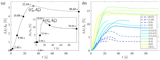
Figure 9.
(a) Temporal evolution of the bed area (main plot) and bed height (inset) variations relative to the initial total bed area and total sediment height , respectively (see text) [ cm, cm, mL/min]. The times indicated for each dot for correspond to the pictures shown in Figure 4c. and are the associated maxima reached at different times and , respectively. (b) Area variation relative to the initial small-grain area, , as a function of time, for different [cm] [ cm, mL/min].
Figure 9b reports the temporal variation of the bed area, , relative to the small-grain layer’s initial area, , for all experiments. This normalization was chosen for two reasons. First, the small-grain layer is the only one always fluidizing in all experiments, therefore contributing mainly to the topography and area variations. Second, the small-grain layer’s height varies in the series with constant, and this variation has to be accounted for when normalizing the area variations. Applying this normalization displays an interesting ordering of the different experiments when varying at constant total sediment height. Starting from a small-grain monolayer and increasing progressively the large grain ratio , we observe a progressive increase in the maximum area which, at the same time, occurs later in time (Figure 9b, dark blue to light blue curves). After reaching an optimum both in the relative area / and in time , both variables decrease. Note that if the times and do not vary depending on the normalization, the value of the maxima varies. For variables relative to the small-grain layer, we will denote the maxima in the area and height and , respectively.
Figure 10a displays the time and corresponding to the maximum in the bed area and height, respectively, as a function of the large-grain percentage, . Both times follow the same trend. They increase while increasing the large-grain layer, until reaching the transition between the regime in which both layers are fluidized, and the percolating regime for the large-grain layer. After this transition, both times decrease. No point is available for %, as no fluidization occurs. The time to reach the maximum area is always larger than the time to reach the maximum sediment height. Figure 10b reports as a function of . Except close to the transition between the two regimes (larger times), which may be subjected to stronger fluctuations, a clear correlation appears between both times, with (dashed line, Figure 10b).
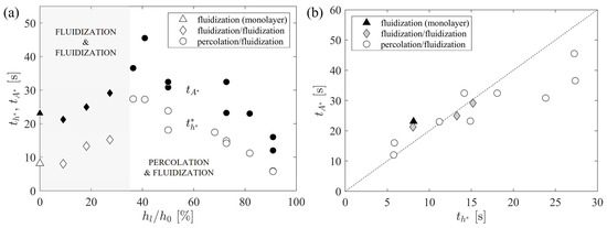
Figure 10.
(a) Time to reach the maximum value of the bed area, (black symbols), and height, (white symbols), as a function of the large-grain percentage, [ cm, mL/min]. (b) vs. . The dashed line indicates slope 2 (see text).
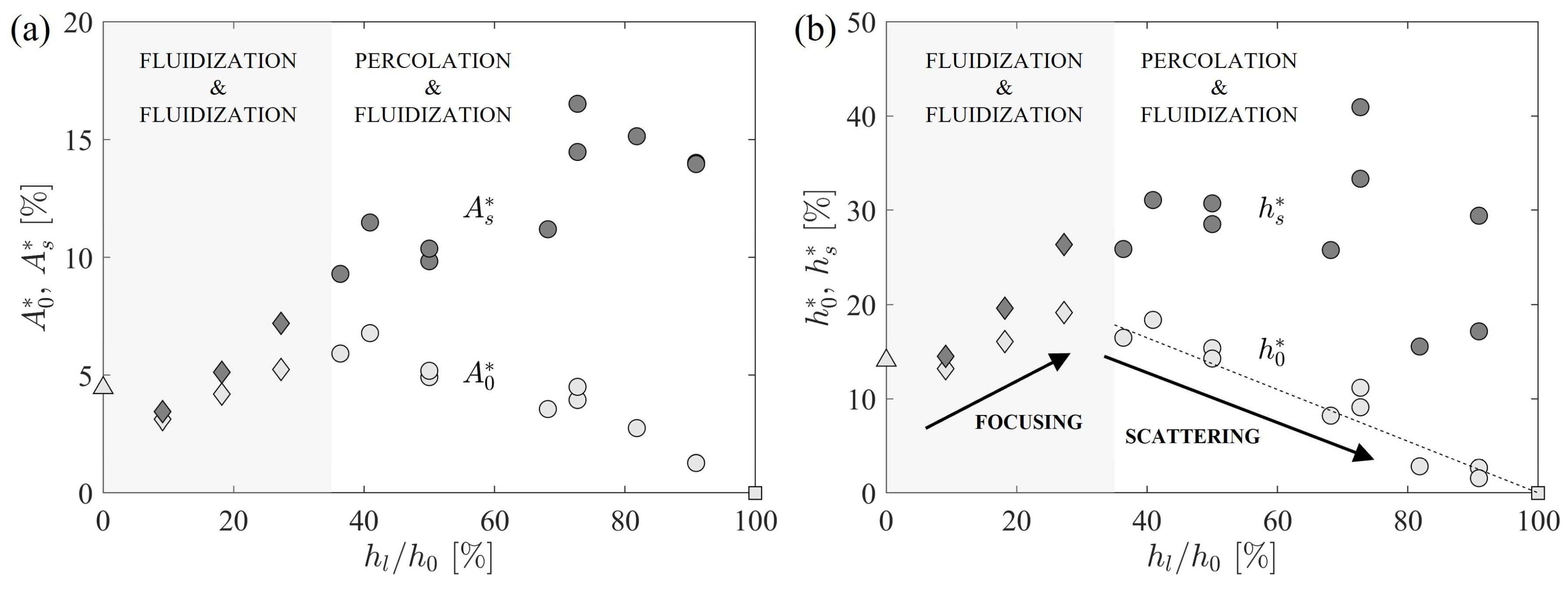
The maximum area and height relative to the initial sediment layer or the small-grain layer are represented in Figure 11 when varying the large-grain percentage. Similarly to their associated time to reach the maximum, and both display a non-monotonous behavior and a maximum value associated with the transition between the fluidization of both layers and the percolation regime for the large grains layer. The existence of this optimum can be interpreted as a focusing vs. scattering effect, which will be discussed in Section 4.2. Interestingly, when considering the area and height variations relative to the small-grain layer, and , no optimum is found, although the data variability strongly increases for large %. These results are further discussed in Section 4.3, wherein we propose a model to explain the decreasing area and height optimum in the percolation and fluidization regime (dashed line, Figure 11) and interpret the existence of an optimum in terms of fluid focusing vs. scattering.
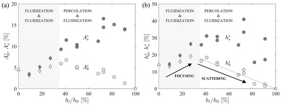
Figure 11.
(a) Maximum bed area relative to the initial sediment height, or to the small-grain area, , as a function of the large grains ratio . (b) Maximum bed height relative to the initial total sediment height, or to the small-grain area, , as a function of the ratio of large grains . The symbols are identical to the ones in Figure 10a. The dashed line represents the model and the black arrows indicate the focusing vs. scattering effect (see Section 4.2) [ cm, mL/min].
4. Discussion
4.1. Invasion Patterns: Transition from Percolation to Fluidization
In this section, we discuss the transition from percolation to fluidization reported for the large-grain layer when decreasing its height (see Section 3.1). Experimentally, for mL/min, the critical height is cm (Figure 5). The order of magnitude of can be retrieved using a simple argument. Following previous erosion parameters introduced in the literature for soil or granular erosion threshold [33,34,35,36], we compare the fluid’s upward velocity, , to the particle settling velocity, . Assuming that the interface between the two layers acts as a secondary source of length , proportional to the large-grain layer height, the flow velocity at the interface is written as follows:
where is the particle volume fraction. This velocity has to be compared to the particle settling velocity. In our experimental conditions, particles are in the inertial regime and their settling velocity is given by [37], as follows:
where kg.m−3 is the difference between the particle and water density, m.s−2 is the gravitational acceleration and is the large grains’ diameter. The flow at the interface manages to lift the large grains, i.e., to overcome the percolation-to-fluidization transition, when , leading to the critical height:
This prediction can only provide a rough estimation, as the particles are strongly polydisperse (Figure 3), while a single particle diameter appears in Equation (3). As is unknown in our system, we use Equation (3) with cm to estimate its order of magnitude. The packing fraction of the large grains was measured by adding a known mass of grains into the cell, %, and we consider the mean and standard deviation of the large grains’ diameter from the particle size distribution (Figure 3a), μm. This gives . This range of values fits reasonably well with the experimental observations, with a secondary source at the interface always smaller than the initial bottom granular layer height. However, this approximation remains rough, as it is based on the settling velocity of a single particle, and considers neither polydispersity (except to infer the error on ) nor collective effects.
4.2. Fluid Focusing vs. Scattering
We discuss here the optimum found for the maximum area and height relative to the initial height, and (Figure 11). To do so, we compare the decompaction front velocity, , to the fluidization velocity (Figure 12). For a monolayer of small grains, which experiences full fluidization, the decompaction front initially propagates upwards at a speed larger than the average fluidization speed of the full layer (Figure 12, black triangle), meaning that the finger which propagates upwards (Figure 4a) decelerates before reaching the top. Introducing a small layer of large grains at the bottom of the system induces a drastic drop both in the decompaction front and in the total fluidization velocities. Whatever the percentage of large grains, as soon as is not null, the decompaction front at the interface exhibits an initial velocity that is lower than the full fluidization velocity (symbols below the dashed line, Figure 12). The decompaction front velocity almost drops to zero close to the transition between the regime in which both layers fluidize (gray region, Figure 12) and the regime in which the fluid always percolates in the large grains. In this second regime, still decreases when increases, while remains roughly constant.
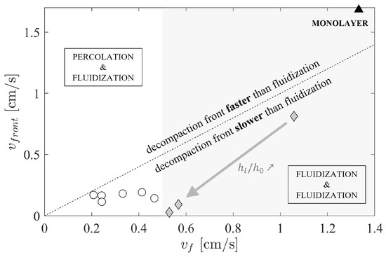
Figure 12.
Decompaction front velocity above the interface as a function of the fluidization velocity of the small grains layer [ cm, mL/min]. The symbols are identical to the ones in Figure 10.
We can interpret these results in terms of fluid propagation. Injecting fluid in a small grains monolayer leads to local fluidization close to the injection nozzle, resulting in the immediate formation of a finger (or “pipe”) propagating upwards. The flow is then well focused up to the free surface. The introduction of a large grains layer at the cell bottom induces fluid percolation at short times in this layer, thus scattering the fluid in the granular matrix, before it meets the interface between both layers. This system can therefore be seen as a monolayer, with a larger effective source at its base (see Figure 4b). The resulting decompaction front propagates upwards and destabilizes to form a finger (pipe), which tends to refocus the flow. This focusing process tends to increase the maximum height and area of the granular bed (black upward arrow, Figure 11b). When the system is not able to fluidize both layers anymore (see Section 4.1), the scattering due to percolation in the large-grain layer and the resulting effective source at the interface becomes too large. The above small-grain layer is not able to refocus the fluid fully before reaching the free surface. The fluid may therefore pierce the free surface not at a single point, but over a wider area (see Figure 4d). The maximum height and area therefore decrease (black downward arrow, Figure 11b).
4.3. Packing Fraction of the Fluidized Region
The decreasing behavior of (black downward arrow, Figure 11b) can be modeled by considering a homogeneous packing fraction in the fluidized region, . Considering an initial packing fraction , it can be written as
where is the maximum (absolute) topography variation.
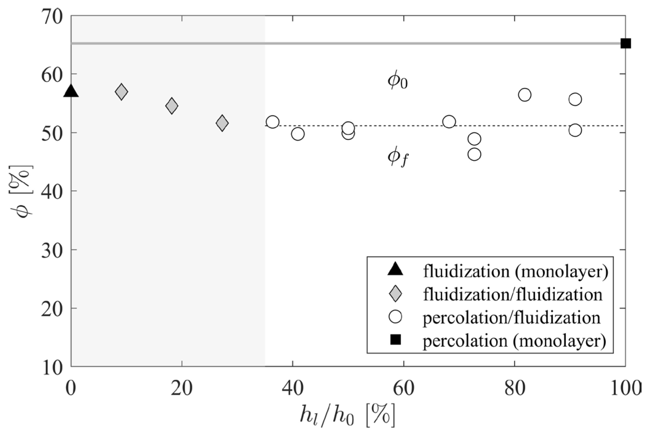
Figure 13 displays the packing fraction in the fluidized region, , for all experiments. We have considered here %, which has been measured directly in the experiments for small grains. In the regime in which only the small-grain layer fluidizes (white region, Figure 13), the packing fraction of the fluidized region remains almost constant, %. Extracting from Equation (4) and considering that gives

Figure 13.
Packing fraction of the granular bed as a function of the percentage of large grains . The initial packing fraction is represented by the gray horizontal line (here %, see text). The symbols represent the packing fraction computed in the small-grain fluidized region, , using Equation (4).
As is roughly constant, Equation (5) states that varies as a decreasing linear function of . Reporting this prediction without any adjustable parameter (dashed line, Figure 11b) provides a good estimation of the decreasing behavior of , which is experimentally reported.
5. Conclusions
Geophysical pipes, which can be seen as focalized fluid migration structures, have been modeled in this work using laboratory experiments in which a fluid is injected at the bottom of a bilayered sediment. This study has demonstrated the drastic effect of the interface between the two sedimentary layers on the system dynamics. In particular, we have underlined the competition between fluid scattering in the bottom layer of coarse grains, due to percolation, and fluid focusing in the above small-grain layer, due to fluidization. The system displays a pipe formation when the focusing effect is stronger than the scattering effect, resulting in a single, localized fluid emission at the sediment’s free surface. These “pipes” do not correspond here to the classical hydrodynamics or industrial definition of a rigid or deformable tube, but display a similar physics of fluid flow, either in a fixed geometry or, in the present case, in a geometry fixed by the system itself by fluid focalization.
The times associated with pipe formation (maximum height and area) exhibit a maximum for a percentage of large grains of about 35%, corresponding to the transition between the two invasion regimes (fluidization of both layers or percolation in the large grains and fluidization in the small-grain layer). This maximum can be interpreted as the largest scattering effect possible in the large grains layer in the regime where both layers fluidize. We cannot explain at present the ratio 2 between the time to reach the maximum area, and the time to reach the maximum height, and further theoretical arguments should be considered to understand this correlation.
The geophysical implications of this work are crucial. It is commonly believed that fluid expulsion at the seafloor is entirely controlled by faults acting as preferential paths for the fluid rising in the sedimentary layer. Here, we have demonstrated that invasion patterns and pipe formation dynamics control the fluid expulsion extent and localization at the seafloor without external driving factors. In addition, we have pointed out the utmost importance of sediments’ composition. Indeed, sediments with a large-grain layer at their bottom, although of relatively small height, may act as a strong “scatterer” of the upward-moving fluid and slow down the pipe formation by decreasing its upward propagation velocity by one or two orders of magnitude. The perspectives for this work are to go further in the modeling of real sedimentary layers by considering multi-layered systems analogue to the geological millefeuille observed in sedimentary basins and introducing possible cohesive effects in the sediments.
Supplementary Materials
The following supporting information can be downloaded at: https://doi.org/10.5281/zenodo.10433274, Video S1: monolayer of small grains [ cm]; Video S2: fluidization of both layers of grains [ cm, cm]; Video S3: percolation in the bottom layer, fluidization of the small grains [ cm, cm]; Video S4: percolation in the bottom layer, fluidization of the small grains [ cm, cm]. For all videos, mL/min (see Figure 4). Note that all movies start at , being the time when the dyed fluid first invades the system.
Author Contributions
Conceptualization, A.G. and V.V.; investigation, G.T. and V.V.; methodology, V.V.; project administration, A.G. and V.V.; funding acquisition: A.G. and V.V.; resources, V.V.; software, G.T. and V.V.; supervision, A.G. and V.V.; validation, A.G., G.T. and V.V.; visualization, A.G. and V.V.; writing—original draft preparation, A.G. and V.V.; writing—review and editing, A.G., G.T. and V.V. All authors have read and agreed to the published version of the manuscript.
Funding
This research received no external funding.
Data Availability Statement
Data are contained within the article and Supplementary Materials.
Acknowledgments
The authors thank two anonymous referees for their pertinent comments which helped to increase the quality of the manuscript.
Conflicts of Interest
The authors declare no conflicts of interest.
References
- Løseth, H.; Wensaas, L.; Arntsen, B.; Hanken, N.-M.; Basire, C.; Graue, K. 1000 m Long Gas Blow-out Pipes. Mar. Pet. Geol. 2011, 28, 1047–1060. [Google Scholar] [CrossRef]
- Cartwright, J.; Santamarina, C. Seismic Characteristics of Fluid Escape Pipes in Sedimentary Basins: Implications for Pipe Genesis. Mar. Pet. Geol. 2015, 65, 126–140. [Google Scholar] [CrossRef]
- Gay, A.; Migeon, S. Geological Fluid Flow in Sedimentary Basins. Bull. Soc. Géol. Fr. 2017, 188, E3. [Google Scholar] [CrossRef]
- Räss, L.; Simon, N.S.C.; Podladchikov, Y.Y. Spontaneous Formation of Fluid Escape Pipes from Subsurface Reservoirs. Sci. Rep. 2018, 8, 11116. [Google Scholar] [CrossRef] [PubMed]
- Gay, A.; Mourgues, R.; Berndt, C.; Bureau, D.; Planke, S.; Laurent, D.; Gautier, S.; Lauer, C.; Loggia, D. Anatomy of a Fluid Pipe in the Norway Basin: Initiation, Propagation and 3D Shape. Mar. Geol. 2012, 332–334, 75–88. [Google Scholar] [CrossRef]
- Hovland, M.; Gardner, J.V.; Judd, A.G. The Significance of Pockmarks to Understanding Fluid Flow Processes and Geohazards. Geofluids 2002, 2, 127–136. [Google Scholar] [CrossRef]
- Svensen, H.; Planke, S.; Malthe-Sørenssen, A.; Jamtveit, B.; Myklebust, R.; Eidem, T.R.; Rey, S.S. Release of Methane from a Volcanic Basin as a Mechanism for Initial Eocene Global Warming. Lett. Nat. 2004, 429, 542–545. [Google Scholar] [CrossRef]
- Svensen, H.; Planke, S.; Chevallier, L.; Malthe-Sørenssen, A.; Corfu, F.; Jamtveit, B. Hydrothermal Venting of Greenhouse Gases Triggering Early Jurassic Global Warming. Earth Planet. Sci. Lett. 2007, 256, 554–566. [Google Scholar] [CrossRef]
- Olsen, J.E.; Skjetne, P. Current Understanding of Subsea Gas Release: A Review. Can. J. Chem. Eng. 2016, 94, 209–219. [Google Scholar] [CrossRef]
- Cardoso, S.S.S.; Cartwright, J.H.E. Increased Methane Emissions from Deep Osmotic and Buoyant Convection beneath Submarine Seeps as Climate Warms. Nat. Commun. 2016, 7, 13266. [Google Scholar] [CrossRef] [PubMed]
- Foschi, M.; Cartwright, J.A.; MacMinn, C.W.; Etiope, G. Evidence for Massive Emission of Methane from a Deep-water Gas Field during the Pliocene. Proc. Natl. Acad. Sci. USA 2020, 117, 27869–27876. [Google Scholar] [CrossRef] [PubMed]
- Gay, A.; Lopez, M.; Berndt, C.; Séranne, M. Geological Controls on Focused Fluid Flow Associated with Seafloor Seeps in the Lower Congo Basin. Mar. Geol. 2007, 244, 68–92. [Google Scholar] [CrossRef]
- Riboulot, V.; Sultan, N.; Imbert, P.; Ker, S. Initiation of Gas-Hydrate Pockmark in Deep-Water Nigeria: Geo-Mechanical Analysis and Modelling. Earth Planet. Sci. Lett. 2016, 434, 252–263. [Google Scholar] [CrossRef]
- Xu, C.; Xu, G.; Xing, J.; Sun, Z.; Wu, N. Research Progress of Seafloor Pockmarks in Spatio-Temporal Distribution and Classification. J. Ocean. Univ. China 2020, 19, 69–80. [Google Scholar] [CrossRef]
- Vidal, V.; Gay, A. Future Challenges on Focused Fluid Migration in Sedimentary Basins: Insight from Field Data, Laboratory Experiments and Numerical Simulations. Pap. Phys. 2022, 14, 140011. [Google Scholar] [CrossRef]
- Nichols, R.J.; Sparks, R.S.J.; Wilson, C.J.N. Experimental Studies of the Fluidization of Layered Sediments and the Formation of Fluid Escape Structures. Sedimentology 1994, 41, 233–253. [Google Scholar] [CrossRef]
- Mourgues, R.; Cobbold, P.R. Some Tectonic Consequences of Fluid Overpressures and Seepage Forces as Demonstrated by Sandbox Modelling. Tectonophysics 2003, 376, 75–97. [Google Scholar] [CrossRef]
- Mörz, T.; Karlik, E.A.; Kreiter, S.; Kopf, A. An Experimental Setup for Fluid Venting in Unconsolidated Sediments: New Insights to Fluid Mechanics and Structures. Sediment. Geol. 2007, 196, 251–267. [Google Scholar] [CrossRef]
- Mazzini, A.; Ivanov, M.K.; Nermoen, A.; Bahr, A.; Bohrmann, G.; Svensen, H.; Planke, S. Complex Plumbing Systems in the near Subsurface: Geometries of Authigenic Carbonates from Dolgovskoy Mound (Black Sea) Constrained by Analogue Experiments. Mar. Pet. Geol. 2008, 25, 457–472. [Google Scholar] [CrossRef]
- Nermoen, A.; Galland, O.; Jettestuen, E.; Fristad, K.; Podladchikov, Y.; Svensen, H.; Malthe-Sørenssen, A. Experimental and Analytic Modeling of Piercement Structures. J. Geophys. Res. 2010, 115, B10202. [Google Scholar] [CrossRef]
- Mourgues, R.; Bureau, D.; Bodet, L.; Gay, A.; Gressier, J.B. Formation of Conical Fractures in Sedimentary Basins: Experiments Involving Pore Fluids and Implications for Sandstone Intrusion Mechanisms. Earth Planet. Sci. Lett. 2012, 313–314, 67–78. [Google Scholar] [CrossRef]
- Luu, L.-H.; Noury, G.; Benseghier, Z.; Philippe, P. Hydro-Mechanical Modeling of Sinkhole Occurrence Processes in Covered Karst Terrains during a Flood. Eng. Geol. 2019, 260, 105249. [Google Scholar] [CrossRef]
- May, F.; Warsitzka, M.; Kukowski, N. Analogue Modelling of Leakage Processes in Unconsolidated Sediments. Int. J. Greenh. Gas Control 2019, 90, 102805. [Google Scholar] [CrossRef]
- Fu, X.; Jimenez-Martinez, J.; Nguyen, T.P.; Carey, J.W.; Viswanathan, H.; Cueto-Felgueroso, L.; Juanes, R. Crustal Fingering Facilitates Free-Gas Methane Migration through the Hydrate Stability Zone. Proc. Natl. Acad. Sci. USA 2020, 117, 31660–31664. [Google Scholar] [CrossRef]
- Yarushina, V.M.; Makhnenko, R.Y.; Podladchikov, Y.Y.; Wang, L.H.; Räss, L. Viscous Behavior of Clay-Rich Rocks and Its Role in Focused Fluid Flow. Geochem. Geophys. Geosyst. 2021, 22, e2021GC009949. [Google Scholar] [CrossRef]
- Montellà, E.P.; Toraldo, M.; Chareyre, B.; Sibille, L. Localized Fluidization in Granular Materials: Theoretical and Numerical Study. Phys. Rev. E 2016, 94, 052905. [Google Scholar] [CrossRef] [PubMed]
- Yarushina, V.M.; Wang, L.H.; Connolly, D.; Kocsis, G.; Fæstø, I.; Polteau, S.; Lakhlifi, A. Focused Fluid-Flow Structures Potentially Caused by Solitary Porosity Waves. Geology 2022, 50, 179–183. [Google Scholar] [CrossRef]
- Gupta, S.; Micallef, A. Modelling the Influence of Erosive Fluidization on the Morphology of Fluid Flow and Escape Structures. Math. Geosci. 2023, 55, 1101–1123. [Google Scholar] [CrossRef]
- Werner, A.D.; Jazayeri, A.; Ramirez-Lagunas, M. Sediment Mobilisation and Release through Groundwater Discharge to the Land Surface: Review and Theoretical Development. Sci. Total Environ. 2020, 714, 136757. [Google Scholar] [CrossRef]
- Warsitzka, M.; Kukowski, N.; May, F. Fluid-Overpressure Driven Sediment Mobilisation and Its Risk for the Integrity for CO2 Storage Sites—An Analogue Modelling Approach. Energy Procedia 2017, 114, 3291–3304. [Google Scholar] [CrossRef]
- Gay, A.; Berndt, C. Cessation/Reactivation of Polygonal Faulting and Effects on Fluid Flow in the Vøring Basin, Norwegian Margin. J. Geol. Soc. Lond. 2007, 164, 129–141. [Google Scholar] [CrossRef]
- Gay, A.; Cavailhès, T.; Grauls, D.; Marsset, B.; Marsset, T. Repeated Fluid Expulsions during Events of Rapid Sea-Level Rise in the Gulf of Lion, Western Mediterranean Sea. Bull. Soc. Géol. Fr. 2017, 188, 24. [Google Scholar] [CrossRef]
- Aderibigbe, O.O.; Rajaratnam, N. Erosion of Loose Beds by Submerged Circular Impinging Vertical Turbulent Jets. J. Hydraul. Res. 1996, 34, 19–33. [Google Scholar] [CrossRef]
- Badr, S.; Gauthier, G.; Gondret, P. Erosion Threshold of a Liquid Immersed Granular Bed by an Impinging Plane Liquid Jet. Phys. Fluids 2014, 26, 023302. [Google Scholar] [CrossRef]
- Vessaire, J.; Varas, G.; Joubaud, S.; Volk, R.; Bourgoin, M.; Vidal, V. Stability of a Liquid Jet Impinging on Confined Saturated Sand. Phys. Rev. Lett. 2020, 124, 224502. [Google Scholar] [CrossRef]
- Alaoui, C.; Gay, A.; Vidal, V. Oscillations of a Particle-Laden Fountain. Phys. Rev. E 2022, 106, 024901. [Google Scholar] [CrossRef]
- Clift, R.; Grace, J.R.; Weber, M.E. Bubbles, Drops and Particles; Academic Press: New York, NY, USA, 1978. [Google Scholar]


Disclaimer/Publisher’s Note: The statements, opinions and data contained in all publications are solely those of the individual author(s) and contributor(s) and not of MDPI and/or the editor(s). MDPI and/or the editor(s) disclaim responsibility for any injury to people or property resulting from any ideas, methods, instructions or products referred to in the content. |
© 2024 by the authors. Licensee MDPI, Basel, Switzerland. This article is an open access article distributed under the terms and conditions of the Creative Commons Attribution (CC BY) license (https://creativecommons.org/licenses/by/4.0/).