On the Use of Different Sets of Variables for Solving Unsteady Inviscid Flows with an Implicit Discontinuous Galerkin Method

Abstract

This article presents a comparison between the performance obtained by using a spatial discretization of the Euler equations based on a high-order discontinuous Galerkin (dG) method and different sets of variables. The sets of variables investigated are as follows: (1) conservative variables; (2) primitive variables based on pressure and temperature; (3) primitive variables based on the logarithms of pressure and temperature. The solution is advanced in time by using a linearly implicit high-order Rosenbrock-type scheme. The results obtained using the different sets are assessed across several canonical unsteady test cases, focusing on the accuracy, conservation properties and robustness of each discretization. In order to cover a wide range of physical flow conditions, the test-cases considered here are (1) the isentropic vortex convection, (2) the Kelvin–Helmholtz instability and (3) the Richtmyer–Meshkov instability.

1. Introduction

The discretization of the Euler equations is traditionally based on conservative variables, but different sets of variables have been proposed in the literature for several reasons [1,2,3]. In fact, even if the use of conservative variables is a natural choice for compressible flows, a discretization based on a different set can possess some interesting and useful properties. One of them is that, when the primitive set of variables is used, the same equations can be discretized for highly compressible and almost incompressible flows [1,2], which is the starting point to obtain a unified numerical approach that is applicable to a wide range of different physical flow conditions. Indeed, the use of primitive variables is historically exploited with the aim to improve the accuracy of the numerical solution of compressible flows in the low Mach number limit, an aspect that has been extensively investigated in the literature for low- [4,5,6] and high-order methods [7,8,9,10,11]. Another useful and less “standard” set of variables are the primitive variables based on the logarithms of pressure and temperature, here named “primitive log”, used to ensure the positivity of all the thermodynamic variables at the discrete level, thus improving the boundedness property of the discretization and, therefore, its robustness. The effect of using this particular set of variables on the behavior of the resulting discretization has been only marginally investigated in [12]. Furthermore, the use of different sets of variables has a strong influence not only on the properties of the numerical discretization (accuracy, conservation and robustness) but even on its overall performance in terms of CPU time, since the choice of a different set can significantly influence the complexity of the scheme. Nevertheless, even if several studies have highlighted the superior performance of the primitive variables with respect to the conservative ones in the past, these studies very often focused on steady solutions in the low Mach number regime, whereas the best choice for unsteady flows ranging from subsonic to hypersonic speeds is less clear, particularly when using high-order methods.

In light of this, the purpose of this article is to highlight the different behaviors of the numerical solution of unsteady inviscid flows when different sets of variables are used in the context of a high-order discretization method both in space and in time. The sets of variables investigated are as follows:

(1)

Conservative variables;

(2)

Primitive variables based on pressure and temperature;

(3)

Primitive variables based on the logarithms of pressure and temperature.

Further, the comparison between them has been focused on the accuracy, conservation and robustness properties of the resulting discretizations.

The spatial approximation of the governing Euler equations is based on a high-order discontinuous Galerkin (dG) method [13], which is very well suited to cope with problems requiring a high-accuracy solution and, thanks to its compact form, for parallel computations.

Furthermore, thanks to its favorable dissipation and dispersion properties, the dG method has been proved to be very effective to solve turbulent flows with both the Direct Numerical Simulation (DNS) [14,15] and the Large Eddy Simulation (LES) [16]. The solution is advanced in time with a high-order linearly implicit Rosenbrock method [17], whose positive performance, in the context of the dG method, has been investigated in [12].

To clearly determine and evaluate the strengths and weaknesses related to the use of each set, an extensive study is carried out presenting the numerical results of several test-cases:

(1)

The isentropic vortex convection problem [18];

(2)

The Kelvin–Helmholtz instability [19,20];

(3)

The Richtmyer–Meshkov instability [21,22].

The isentropic vortex is a very well known test-case with an exact analytical solution, here used to assess accuracy and conservation properties of the investigated discretizations for a wide range of different physical flow conditions. The robustness of the discretizations will also be investigated, focusing the attention on flow problems that present values of the thermodynamic variables close to zero. The Kelvin–Helmholtz and the Richtmyer–Meshkov instabilities are characterized by complex mixing layers and are here used to further determine the robustness property of the discretizations. For the three aforementioned test-cases, several time refinement studies have been carried out by using different dG polynomial approximations, several grids and different physical flow conditions.

In Section 2, the governing equations are presented. Section 3 briefly describes the spatial (dG method) and temporal (Rosenbrock-type scheme) discretizations used. In Section 4, we show the results of the numerical experiments. Findings and conclusions are summarized in the Section 5.

2. The Governing Equations

The equations governing the behavior of inviscid compressible flows, i.e., the Euler equations, can be written via Einstein’s notation as follows:

$$\begin{array}{cc}\hfill & {\displaystyle \frac{\partial \rho }{\partial t}}+{\displaystyle \frac{\partial }{\partial x_j}}\left(\rho u_j\right)=0,\hfill \\ \hfill & {\displaystyle \frac{\partial }{\partial t}}\left(\rho u_i\right)+{\displaystyle \frac{\partial }{\partial x_j}}\left(\rho u_j{u}_i\right)=-{\displaystyle \frac{\partial p}{\partial x_i}},\hfill \\ \hfill & {\displaystyle \frac{\partial }{\partial t}}\left(\rho E\right)+{\displaystyle \frac{\partial }{\partial x_j}}\left(\rho u_{j}H\right)=0.\hfill \end{array}$$

(1)

In these equations, $\rho$ is the fluid density; p is the pressure; $\mathbf{u}=\{u_1,\dots ,u_d\}$ is the velocity vector; E and H are the total energy and enthalpy, respectively; and $i,j=1,\cdots ,d$, where d is the number of geometrical dimensions. For a perfect gas, $p=\left(\gamma -1\right)\rho \left[E-\left(u_i{u}_i\right)/2\right]$, where $\gamma =c_p/c_v$ is the ratio of gas-specific heats, here equal to $1.4$.

System (1) can be written in compact form as

$${\displaystyle \frac{\partial \mathbf{q}}{\partial t}}+{\displaystyle \frac{\partial {\mathbf{F}}_i\left(\mathbf{q}\right)}{\partial x_i}}=\mathbf{0},$$

(2)

where $\mathbf{q}=\{\rho ,\rho u_i,\rho E\}$ is the vector of conservative variables and $\mathbf{F}\in {\mathbb{R}}^{2+d}\otimes {\mathbb{R}}^d$ is the convective flux.

If we consider now a generic set of variables $\mathbf{v}\in {\mathbb{R}}^{2+d}$, here named the set of working variables, Equation (2) can be written as

$$\mathbf{P}\left(\mathbf{v}\right){\displaystyle \frac{\partial \mathbf{v}}{\partial t}}+{\displaystyle \frac{\partial {\mathbf{F}}_i\left(\mathbf{v}\right)}{\partial x_i}}=\mathbf{0},$$

(3)

where $\mathbf{P}\left(\mathbf{v}\right)=\partial \mathbf{q}\left(\mathbf{v}\right)/\partial \mathbf{v}\in {\mathbb{R}}^{2+d}\otimes {\mathbb{R}}^{2+d}$ is the matrix that takes into account the change in variables from the conservative set $\mathbf{q}$ to the generic set $\mathbf{v}$ and that it reduces to identity matrix $\mathbf{I}$ if the set of working variables is the conservative one. In the following list, the sets of working variables investigated here are reported:

• Conservative variables: $\mathbf{v}=\{\rho ,\rho u_i,\rho E\}$;
• Primitive variables: $\mathbf{v}=\{p,u_i,T\}$;
• Primitive log variables: $\mathbf{v}=\{log\left(p\right),u_i,log\left(T\right)\}$.

Above, T is the temperature. Note that, when primitive log variables are used, pressure and temperature values, computed as $p=e^{log\left(p\right)}$ and $T=e^{log\left(T\right)}$, are always positive. Therefore, the definition of primitive log variables ensures the positivity of all the thermodynamic variables at discrete level—a property that is very useful to obtain a better robustness of the numerical modeling, especially when these variables assume values near to zero or in case of strong shock oscillations.

3. Space and Time Discretization

In what follows, we briefly describe the main features of the methods used to perform the spatial (dG) and temporal (Rosenbrock) discretizations of Equation (3). For a more exhaustive overview and treatment concerning dG methods, the interested reader is referred to [13] and the references cited therein. For an efficient implementation of Rosenbrock schemes when different sets of working variables are used, the reader can refer to [12] for further details in this regard and for the values of the coefficients necessary for its implementation.

3.1. The Discontinuous Galerkin Method

We denote with ${\mathcal{K}}_h=\left\{K\right\}$ a discretization of the computational domain ${\mathsf{\Omega }}_h\in {\mathbb{R}}^d$, consisting of non-overlapping elements K such that

$${\mathsf{\Omega }}_h=\bigcup _{K\in {\mathcal{K}}_h}K,$$

(4)

and we define a discrete polynomial space in physical (mesh) coordinates:

$${\mathbb{P}}_d^k\left({\mathcal{K}}_h\right)\stackrel{\mathrm{def}}{=}\left\{v_h\in L^2\left(\mathsf{\Omega }\right)|v_{h|K}\in {\mathbb{P}}_d^k\left(K\right),\forall K\in {\mathcal{K}}_h\right\},$$

(5)

where k is a non-negative integer and ${\mathbb{P}}_d^k\left(K\right)$ denotes the restriction to K of the polynomial functions of d variables and total degree $\le k$.

The weak formulation of Equation (3) is obtained by multiplying it by an arbitrary smooth test function $\mathbf{w}=\{w_1,\cdots ,w_{2+d}\}$ and integrating by the following parts:

$${\int }_{{\mathsf{\Omega }}_h}\mathbf{w}·\left(\mathbf{P}\left(\mathbf{v}\right){\displaystyle \frac{\partial \mathbf{v}}{\partial t}}\right)d\mathsf{\Omega }-{\int }_{{\mathsf{\Omega }}_h}\nabla \mathbf{w}:\mathbf{F}\left(\mathbf{v}\right)d\mathsf{\Omega }+{\int }_{\partial {\mathsf{\Omega }}_h}\mathbf{w}\otimes \mathbf{n}:\mathbf{F}\left(\mathbf{v}\right)d\sigma =\mathbf{0},$$

(6)

where the : symbol is the double dot product that calculates the sum of the products of the corresponding components of the two tensors; the ⊗ symbol represents the outer product of vectors $\mathbf{w}$ and $\mathbf{n}$, resulting in a tensor; and $\mathbf{n}$ is the outward unit normal vector to the boundary of the computational domain $\partial {\mathsf{\Omega }}_h$. To discretize Equation (6), we replace the solution $\mathbf{v}$ with a finite element approximation ${\mathbf{v}}_h$ and the test function $\mathbf{w}$ with a discrete test function ${\mathbf{w}}_h$, both belonging to the discrete space ${\mathbf{V}}_h\stackrel{\mathrm{def}}{=}{\left[{\mathbb{P}}_d^k\left({\mathcal{K}}_h\right)\right]}^{2+d}$. Each component $v_{h,j}$, $j=1,\cdots ,2+d$ of the numerical solution ${\mathbf{v}}_h\in {\mathbf{V}}_h$ can be expressed, in terms of the elements of the global vector $\mathbf{V}$ of unknown degrees of freedom, as $v_{h,j}={\varphi }_l{V}_{j,l}$, $l=1,\cdots ,N_{dof}=\left({\displaystyle \genfrac{}{}{0pt}{}{k-1}{d}}\right)$, $\forall K\in {\mathcal{K}}_h$, where ${\varphi }_l$ belongs to the set of basis functions defined on each element of the mesh.

Furthermore, we define the set ${\mathcal{F}}_h$ of the mesh faces ${\mathcal{F}}_h\stackrel{\mathrm{def}}{=}{\mathcal{F}}_h^i\cup {\mathcal{F}}_h^b$, where ${\mathcal{F}}_h^b$ collects the faces located on $\partial {\mathsf{\Omega }}_h$ and ${\mathcal{F}}_h^i$ collects the internal faces F. For any $F\in {\mathcal{F}}_h^i$, there exist two elements $K^{+},K^{-}\in {\mathcal{K}}_h$ such that $F\in \partial K^{+}\cap \partial K^{-}$. Moreover, for all $F\in {\mathcal{F}}_h$, ${\mathbf{n}}_F=\left\{n_i\right\}$ with $i=1,\cdots ,d$ is the uniquely defined normal unit vector pointing from $K^{+}$ to $K^{-}$. Note that, when the face is located on the boundary, ${\mathbf{n}}_F$ coincides with the vector $\mathbf{n}$ already defined. Finally, as a function $w_h\in {\mathbb{P}}_d^k\left({\mathcal{K}}_h\right)$ is double valued over an internal face $F\in {\mathcal{F}}_h^i$, we introduce the jump trace operator $\left[\left[w_h\right]\right]\stackrel{\mathrm{def}}{=}{w_h}_{|K^{+}}-{w_h}_{|K^{-}}$ that acts component-wise when applied to a vector.

The dG discretization of the Euler equations consists in seeking, for $j=1,\cdots ,2+d$, the elements of ${\mathbf{v}}_h$ such that

$$\sum _{K\in {\mathcal{K}}_h}{\int }_K{\varphi }_i{P}_{j,k}\left({\mathbf{v}}_h\right){\varphi }_l{\displaystyle \frac{d{V}_{k,l}}{dt}}d\mathbf{x}-\sum _{K\in {\mathcal{K}}_h}{\int }_K{\displaystyle \frac{\partial {\varphi }_i}{\partial x_n}}{F}_{j,n}\left({\mathbf{v}}_h\right)d\mathbf{x}+\sum _{F\in {\mathcal{F}}_h}{\int }_F\left[\left[{\varphi }_i\right]\right]{\widehat{F}}_j\left({\mathbf{v}}_h^{\pm },{\mathbf{n}}_F\right)d\mathbf{x}=\mathbf{0},$$

(7)

for $i=1,\cdots ,N_{dof}$, where repeated indices imply summation over the ranges $k=1,\cdots ,2+d$, $l=1,\cdots ,N_{dof}$ and $n=1,\cdots ,d$.

In the above equations, at each face $F\in {\mathcal{F}}_h$, we denote with $\widehat{F_j}$ the jth-component of the convective numerical flux, which can be any numerical flux commonly considered in the Finite Volume Method context. In this work, the Godunov flux has been used, i.e., the physical flux computed using the exact iterative Riemann solver of Gottlieb and Groth [23], which is a provable entropy stable flux [24]. The integrals are evaluated by means of Gaussian quadrature formulae with degree of exactness $k^q=2k+1$, which corresponds to ${\lceil (k^q+1)/2\rceil }^d$ quadrature points and guarantees the exact volume and surface integration of polynomials of order $2k$.

3.2. The Linearly Implicit Rosenbrock Method

After that, Equation (7) is numerically integrated in space via the dG method—the system of equations that, following the Method of Lines (MOL), must be further discretized in time, can be written as

$${\mathbf{M}}_{\mathbf{P}}\left(\mathbf{V}\right){\displaystyle \frac{d\mathbf{V}}{dt}}=\mathbf{R}\left(\mathbf{V}\right).$$

(8)

In the above equation, $\mathbf{V}$ is the global vector of unknown degrees of freedom, $\mathbf{R}\left(\mathbf{V}\right)$ is the global vector of residuals resulting from the integrals of the dG discretized differential operators in Equation (7) and ${\mathbf{M}}_{\mathbf{P}}\left(\mathbf{V}\right)$ is a global block matrix. In this work, thanks to the use of orthonormal basis functions defined in the physical space [25], ${\mathbf{M}}_{\mathbf{P}}$ reduces to the identity matrix for the conservative set of variables; meanwhile, for a different set, the transformation matrix $\mathbf{P}$ couples the degrees of freedom of the variables ${\mathbf{v}}_h$ within each block of ${\mathbf{M}}_{\mathbf{P}}$ and, therefore, ${\mathbf{M}}_{\mathbf{P}}$ is no longer a diagonal matrix. Please note that, even if the evaluation of CPU times obtained using different sets of variables is beyond the scope of this article, this factor significantly impacts computational efficiency. Specifically, the use of conservative variables greatly reduces computational cost compared to other variable sets.

To advance the solution in time by using an s stages Rosenbrock scheme, we must solve

$${\mathbf{V}}^{n+1}={\mathbf{V}}^n+\sum _{j=1}^s{m}_j{\mathbf{Y}}_j,$$

(9)

$${\left({\displaystyle \frac{\mathbf{I}}{\gamma \Delta t}}+\tilde{\mathbf{J}}\right)}^n{\mathbf{Y}}_i=-\tilde{\mathbf{R}}\left({\mathbf{V}}^n+\sum _{j=1}^{i-1}{a}_{ij}{\mathbf{Y}}_j\right)+\sum _{j=1}^{i-1}{\displaystyle \frac{c_{ij}}{\Delta t}}{\mathbf{Y}}_j,i=1,\cdots ,s,$$

(10)

where, omitting the dependence on $\mathbf{V}$ for notational convenience,

$$\mathbf{J}={\displaystyle \frac{\partial \mathbf{R}}{\partial \mathbf{V}}},\tilde{\mathbf{R}}={\mathbf{M}}_{\mathbf{P}}^{-1}\mathbf{R},\tilde{\mathbf{J}}={\displaystyle \frac{\partial \tilde{\mathbf{R}}}{\partial \mathbf{V}}}={\mathbf{M}}_{\mathbf{P}}^{-1}\left(\mathbf{J}-{\displaystyle \frac{\partial {\mathbf{M}}_{\mathbf{P}}}{\partial \mathbf{V}}}\tilde{\mathbf{R}}\right),$$

(11)

and $m_j$, $a_{ij}$ and $c_{ij}$ are real coefficients. Among all the possible Rosenbrock schemes, in this work is used the three stages, order three, scheme of Lang and Verwer [17].

The linear systems arising from the use of this time integration method are solved with the GMRES method preconditioned with an ILU(0) decomposition applied on each mesh partition, i.e., the preconditioning matrix of each mesh partition has the same level of fill of the original matrix. The GMRES method and the ILU(0) decomposition are carried out using the PETSc library (Portable, Extensible Toolkit for Scientific Computation) [26], and the PETSc interface to the MPI library was used to perform parallel computations. The simulations were performed using two different computational resources: some were run on a system with two sixteen-core AMD Opteron 6276 CPUs, while others were executed on the Leonardo supercomputer at CINECA, which is equipped with state-of-the-art hardware including multiple high-performance cores optimized for parallel computing.

4. Numerical Results

In this section, the behavior of the resulting numerical discretizations arising from the use of the sets of working variables investigated is shown. In particular, the performance of these discretizations will be assessed based on the accuracy of their solutions, as well as their conservation and robustness properties, across various dG polynomial approximations, grid resolutions and flow conditions. In particular, the dG approximations investigated in this work are ${\mathbb{P}}^3$ and ${\mathbb{P}}^6$, selected to evaluate how different dG accuracy levels affect the behavior of the numerical discretizations. To this end, the following test-cases have been used:

• The isentropic vortex (Section 4.1);
• The Kelvin–Helmholtz instability (Section 4.2);
• The Richtmyer–Meshkov instability (Section 4.3).

For the isentropic vortex, which has an analytical solution, an extensive assessment has been conducted for different dG polynomial approximations, evaluating the accuracy and the conservation properties of the different discretizations in terms of $\eta$ and $\epsilon$ errors, respectively. These two indicators have been defined as

$$\begin{array}{cc}\eta (\circ ,{•}_{ref})\hfill & ={\left({\mathsf{\Omega }}_h\right)}^{-1/2}\left|\right|\circ -{•}_{ref}{\left|\right|}_{L^2},\hfill \\ \epsilon (\circ ,{•}_{ref})\hfill & ={\mathsf{\Omega }}_h^{-1}\left|\left({\int }_{{\mathsf{\Omega }}_h}\circ d\mathsf{\Omega }-{\int }_{{\mathsf{\Omega }}_h}{•}_{ref}d\mathsf{\Omega }\right)\right|,\hfill \end{array}$$

(12)

where ∘ and ${•}_{ref}$ are the numerical and the “reference” solutions, respectively, with the latter being equal to the $L_2$–projection of the initial solution on the dG polynomial space. In particular, the $\eta$ errors will be computed for pressure, temperature and velocity components and, to evaluate the global conservation properties of entropy, kinetic energy and enstrophy, the $\epsilon$ errors will be computed for $\rho s$, k and $\zeta$ quantities, which are defined as

$$\begin{array}{cc}\rho s\hfill & =\rho ln\left(p{\rho }^{-\gamma }\right),\hfill \\ k\hfill & =\rho \left({\displaystyle \frac{u_1^2+u_2^2}{2}}\right),\hfill \\ \zeta \hfill & ={\displaystyle \frac{1}{2\rho }}{\left({\displaystyle \frac{\partial u_2}{\partial x_1}}-{\displaystyle \frac{\partial u_1}{\partial x_2}}\right)}^2.\hfill \end{array}$$

(13)

Finally, the robustness of the discretizations will be evaluated considering different flow conditions, i.e., low and high Mach numbers (even in case of their simultaneous occurrence) and values of the thermodynamic variables near to zero.

The results of the simulations performed for the Kelvin–Helmholtz (KH) and the Richtmyer–Meshkov (RM) instabilities will further assess the robustness of the different discretizations for non-smooth problems characterized by complex mixing layers and shock interaction. For these physical flow conditions, the robustness property will be evaluated, not only varying the dG approximation but even for a wide range of Atwood numbers (KH) and for different grid resolutions (RM).

For all the simulations reported here, the GMRES parameters, used by the Rosenbrock scheme, are an iterative linear solver tolerance equal to ${10}^{-12}$ to minimize the temporal discretization error for any used time step and a maximum number of Krylov-subspace vectors equal to 120 with a number of restarts equal to 1.

4.1. The Isentropic Vortex Convection

In this section, we consider the convection of an inviscid isentropic vortex [18]. In particular, we will evaluate the performance, given by the working sets of variables, for the convection of different isentropic vortices added to different mean flows. For this reason, in what follows, the results of this test-case have been split between the case with a perturbation proportional to the free-stream flow (Section 4.1.1) and the case with a perturbation that is not proportional to it (Section 4.1.2).

In both cases, the computational domain is $0\le x_i\le L$, with $L=10$, which is discretized with a uniform grid made of $25\times 25$ quadrilateral elements. All boundary conditions are periodic and the simulations are performed using several time step sizes $\Delta t=t_f/n_{cyc}$. In the above formula $n_{cyc}$ is the total number of iterations necessary to reach the non-dimensional final time $t_f=10$, which corresponds to the time necessary by the vortex to complete one revolution. The dG approximations used are ${\mathbb{P}}^3$ and ${\mathbb{P}}^6$.

4.1.1. Vortex 1: Perturbation Proportional to the Free-Stream Flow

The initial flow conditions of this test case are given by

$$\begin{array}{cc}{u}_1\hfill & =U-{\displaystyle \frac{\alpha M_{\infty }}{2\pi }}\left(x_2-{\displaystyle \frac{L}{2}}\right)e^{\beta \left(1-r^2\right)},\hfill \\ u_2\hfill & =U+{\displaystyle \frac{\alpha M_{\infty }}{2\pi }}\left(x_1-{\displaystyle \frac{L}{2}}\right)e^{\beta \left(1-r^2\right)},\hfill \\ T\hfill & =1-{\displaystyle \frac{{\left(\alpha M_{\infty }\right)}^2\left(\gamma -1\right)}{16\beta \gamma {\pi }^2}}{e}^{2\beta \left(1-r^2\right)},\hfill \\ p\hfill & ={\left(1-{\displaystyle \frac{{\left(\alpha M_{\infty }\right)}^2\left(\gamma -1\right)}{16\beta \gamma {\pi }^2}}{e}^{2\beta \left(1-r^2\right)}\right)}^{{\displaystyle \frac{\gamma }{\gamma -1}}},\hfill \end{array}$$

where U are the free-stream non-dimensional velocity components and r is the distance of a generic point of the computational domain with respect to the vortex center, which is initially placed in the middle of the grid. The $\alpha$ and $\beta$ values are set equal to $5/\sqrt{2}$ and $1/2$, respectively. In particular, several U values, corresponding to different “free-stream” Mach numbers, have been considered in order to highlight the behavior of the numerical solution for high and low Mach number flows. The “free-stream” Mach numbers investigated are as follows:

(a)

$M_{\infty }\simeq 1.4·{10}^{-3}$;

(b)

$M_{\infty }\simeq 1.4$;

(c)

$M_{\infty }\simeq 2.7$.

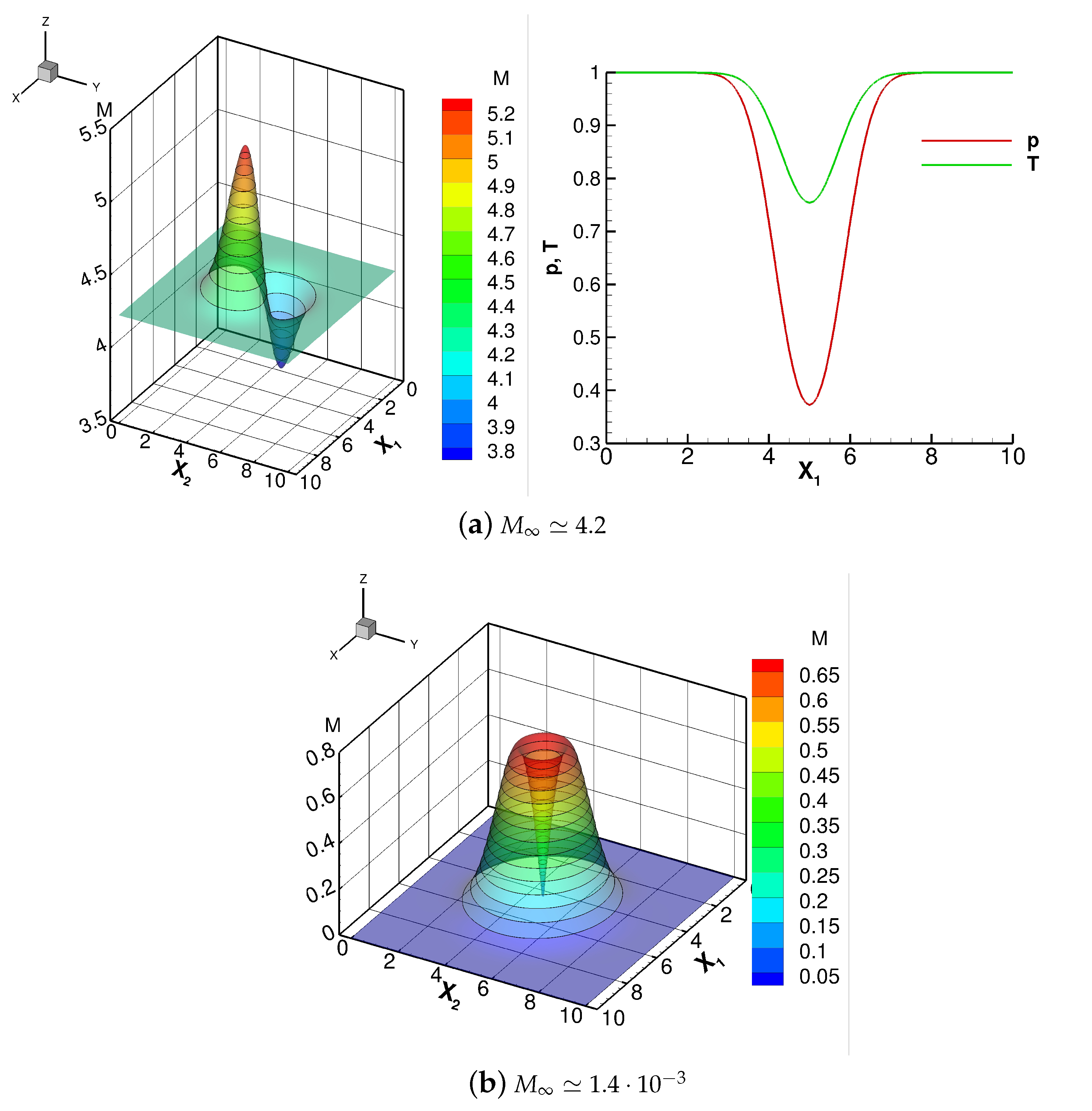
Figure 1 shows the Mach number contours at time $t=0$ for the above three cases. Note that the first case corresponds to a very low Mach number flow, the second one considers a transonic/supersonic Mach number range and the last one a supersonic/hypersonic Mach number range. Furthermore, for $M_{\infty }\simeq 2.7$, the right plot in Figure 1c shows the values of pressure and temperature along the center-line $x_2=5$. For this case, we want to put in evidence that the min values of the thermodynamic variables—that occur in the middle of the computational domain—are near to zero, especially as they concern the pressure. In particular, $p_{min}\simeq 5·{10}^{-4}$ and $T_{min}\simeq 1.1·{10}^{-1}$.

Figure 2 shows the results of the time refinement study, performed for all the sets of variables investigated here, using ${\mathbb{P}}^3$ and ${\mathbb{P}}^6$ dG approximations. Overall, we can notice that, while little differences can be noticed for $M_{\infty }\simeq 1.4·{10}^{-3}$ and $M_{\infty }\simeq 1.4$ in terms of robustness, the plots in the last column, which refer to $M_{\infty }\simeq 2.7$, show a very different behavior depending on the set of variables used. In particular, thanks to the use of the logarithms of pressure and temperature, which ensure the positivity of these quantities at the discrete level, the primitive log variables are more robust. Note, in fact, that by using the primitive log variables it is possible to perform convergent solutions with both the dG approximations, even for relatively large time step sizes. Furthermore, this set is the only one that is able to give a discretization that does not “blow up” with the ${\mathbb{P}}^3$ dG approximation (the results of primitive and conservative sets of variables and ${\mathbb{P}}^3$ approximation are not shown in the plots in Figure 2c since their use leads to a divergent solution). Concerning the accuracy of the solution, what we can conclude is that for $M_{\infty }\simeq 1.4·{10}^{-3}$ and both the dG approximations considered here, there are only some little differences for the temperature when the spatial accuracy is not achieved, with both the primitive sets that outperform the conservative one. For $M_{\infty }\simeq 1.4$, the differences become more evident, especially for the temperature and for the two velocity components when a time step size small enough to let the spatial discretization errors show up is used. For $M_{\infty }\simeq 2.7$, these differences become larger for all the variables considered here.

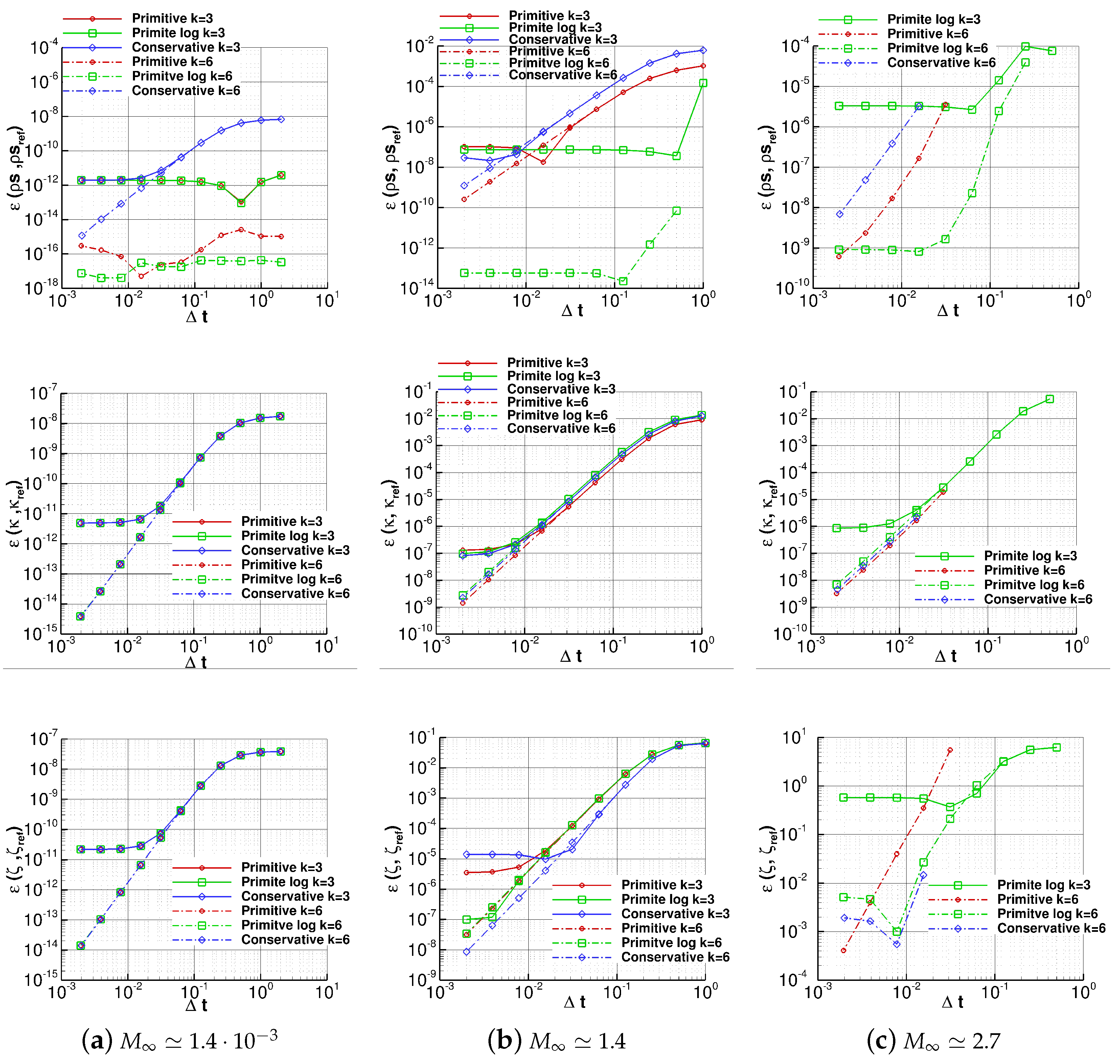
In Figure 3, we report the $\epsilon$ errors of $\rho s$, $\kappa$ and $\zeta$. Looking at the middle row of the figure, we can notice that the $\epsilon$ values of k are more or less independent from the set of variables used, while the same values computed for $\zeta$ and reported at the bottom row of the figure show larger differences for $M_{\infty }\simeq 1.4$ and, to a greater extent, for $M_{\infty }\simeq 2.7$. Finally, by looking at the top row of the figure, the plots show that the $\epsilon$ errors of $\rho s$ computed with the primitive log variables reach the plateau values for very large time step sizes with both ${\mathbb{P}}^3$ and ${\mathbb{P}}^6$ approximations and all the “free-stream” Mach numbers investigated.

4.1.2. Vortex 2: Equal Perturbation for Different Free-Stream Flows

The initial flow conditions of this test case are given by

$$\begin{array}{cc}{u}_1\hfill & =U-{\displaystyle \frac{\alpha }{2\pi }}\left(x_2-{\displaystyle \frac{L}{2}}\right)e^{\beta \left(1-r^2\right)},\hfill \\ u_2\hfill & =U+{\displaystyle \frac{\alpha }{2\pi }}\left(x_1-{\displaystyle \frac{L}{2}}\right)e^{\beta \left(1-r^2\right)},\hfill \\ T\hfill & =1-{\displaystyle \frac{{\alpha }^2\left(\gamma -1\right)}{16\beta \gamma {\pi }^2}}{e}^{2\beta \left(1-r^2\right)},\hfill \\ p\hfill & ={\left(1-{\displaystyle \frac{{\alpha }^2\left(\gamma -1\right)}{16\beta \gamma {\pi }^2}}{e}^{2\beta \left(1-r^2\right)}\right)}^{{\displaystyle \frac{\gamma }{\gamma -1}}},\hfill \end{array}$$

where U, r and $\beta$ values are equal to the ones already defined in the previous section. The $\alpha$ parameter, which determines the strength of the vortex added to the free-stream, is set to 5. The “free-stream” Mach numbers investigated in this case are

(a)

$M_{\infty }\simeq 4.2$;

(b)

$M_{\infty }\simeq 1.4·{10}^{-3}$.

Figure 4 shows the Mach number contours at time $t=0$ and, in the right plot Figure 4a, the values of pressure and temperature along the center-line $x_2=5$ for $M_{\infty }\simeq 4.2$. We want to underline that case (a), as case (c) of the previous section, has a supersonic/hypersonic Mach number range, but the min values of the thermodynamic variables are quite far from a zero value. Finally, note that case (b) presents a very wide Mach number range with $M\in \left[1.4·{10}^{-3},0.71\right]$.

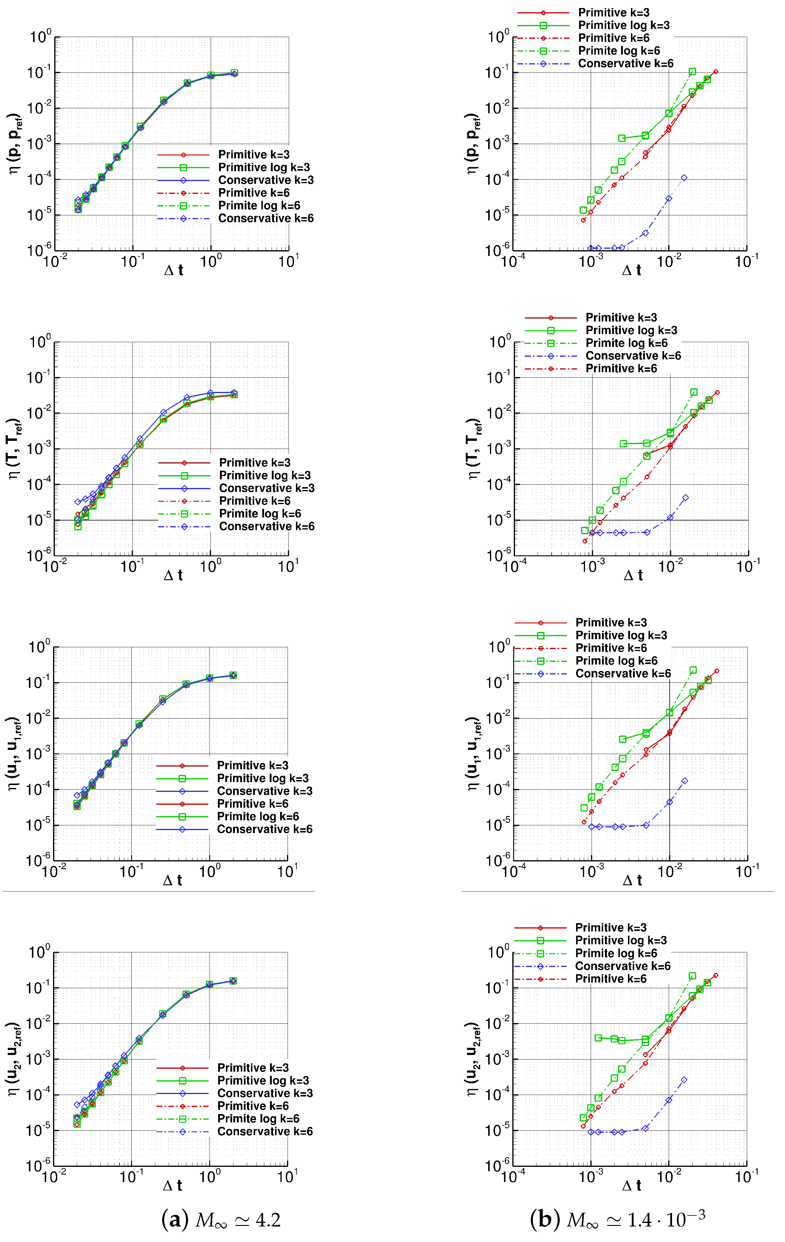
Figure 5 reports the results of the time refinement study, performed for all the sets of variables investigated here, using ${\mathbb{P}}^3$ and ${\mathbb{P}}^6$ dG approximations. Overall, we can notice that, while little differences in terms of accuracy or robustness can be noticed for $M_{\infty }\simeq 4.2$, the plots that refer to $M_{\infty }\simeq 1.4·{10}^{-3}$ show a very different behavior of the numerical solution depending on the set of variables used. The results for this low Mach number “free-stream” flow show that the choice of the set of working variables has a deep influence on the accuracy of the solution and on the robustness of the related discretization. The conservative set is the less robust, with divergent solutions for the ${\mathbb{P}}^3$ dG approximation for all the time step sizes investigated (note that, in the plots, the results related to this Mach number and this set of variables are not reported). Nevertheless, concerning the accuracy, when raising the dG approximation up to ${\mathbb{P}}^6$, the conservative variables give much better results for a fixed time step size with respect to all the other sets of variables; this is especially for large time steps, since the plateau value is immediately reached.

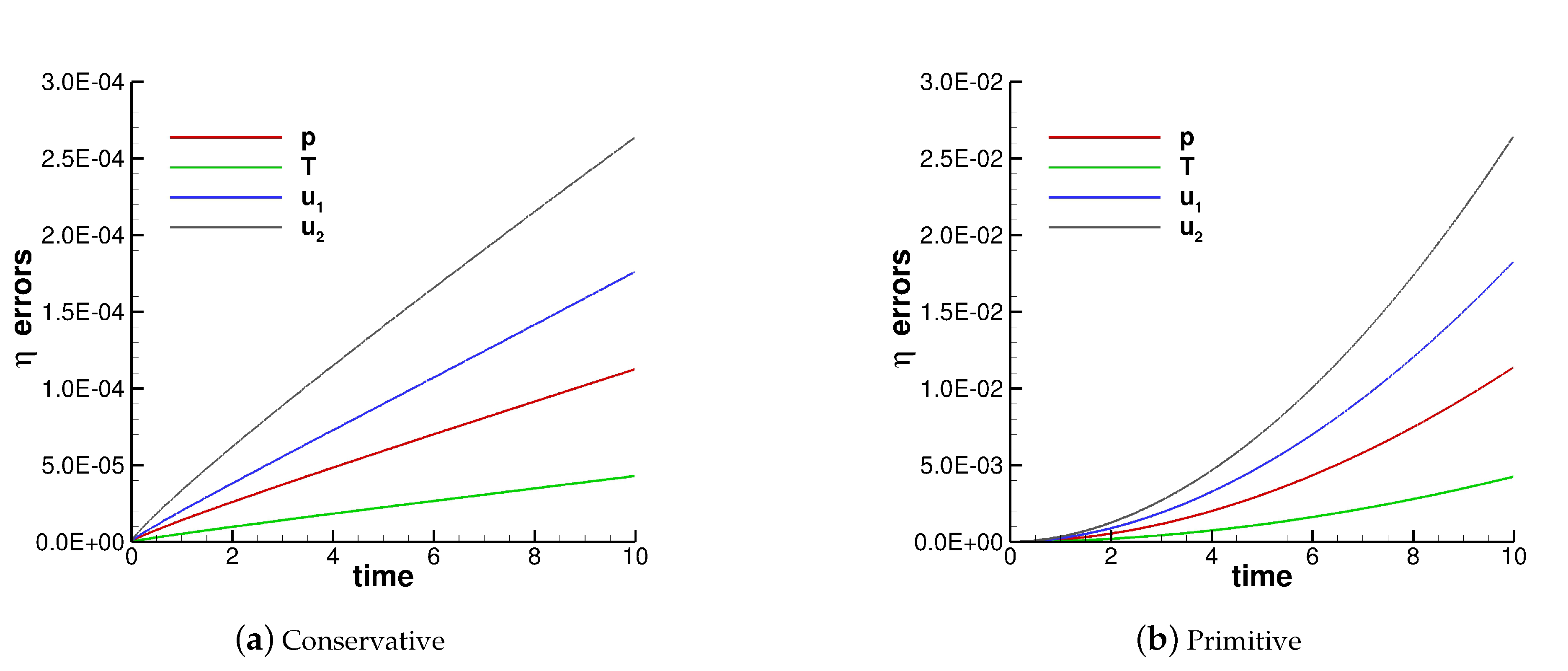
To further investigate this behavior, we analyzed the growth of errors over time for both the conservative and primitive sets of variables, as shown in Figure 6. Note that, since the analytical solution of this problem corresponds to a pure advection of the vortex at the free-stream velocity, we can compute the $\eta$ errors for any simulation time. The two plots of the figure show that the conservative set has a linear error growth while the error grows quadratically using the primitive set. These results are in agreement with the findings reported by H. Ranocha et al. [27]. In fact, in this article, the results of the discretization of several nonlinear dispersive wave equations have shown that the error grows quadratically in time for numerical methods that do not conserve energy and grows only linearly for methods that conserve energy up to rounding errors.

4.2. The Kelvin–Helmholtz Instability Problem

This section deals with the two-dimensional inviscid Kelvin–Helmholtz (KH) instability problem [19,20]. KH-type flows are known to be very sensitive to initial conditions as well as to the numerical resolution and small perturbations. Indeed, the flow evolution is characterized by the generation of small structures becoming increasingly smaller upon enhancement of space and time numerical resolution.

The test case is governed by the Atwood number $A=\left({\rho }_2-{\rho }_1\right)/\left({\rho }_2+{\rho }_1\right)$, which quantifies the instability-driving force, and initialized according to the parameterization provided in the works of Rueda et al. [19] and Chan et al. [20] as

$$\begin{array}{cc}\hfill & u_1=U\left(f\left(x_2\right)-{\displaystyle \frac{1}{2}}\right),\hfill \\ \hfill & u_2={\displaystyle \frac{U}{10}}sin\left(2\pi x_1\right),\hfill \\ \hfill & p=1,\hfill \\ \hfill & \rho ={\rho }_1+f\left(x_2\right)\left({\rho }_2-{\rho }_1\right),\hfill \end{array}$$

(14)

where

$$\begin{array}{cc}\hfill & U=\sqrt{{\displaystyle \frac{p}{{\rho }_1}}},\hfill \\ \hfill & {\rho }_1=1,\hfill \\ \hfill & f\left(x_2\right)={\displaystyle \frac{1}{2}}[tanh(15x_2+7.5)-tanh(15x_2-7.5)],\hfill \end{array}$$

(15)

with $f\left(x_2\right)$ acting as a smoothing function to avoid field discontinuities.

The domain size is set as $-1\le x_i\le 1$ with periodic boundary conditions and discretized by using a $32\times 32$ uniform Cartesian grid. To test the robustness of the numerical schemes resulting from different sets of working variables, the Atwood number has been varied in the range $0.3\le A\le 0.75$ and the simulations are performed up to a final time $t_f=20$ using dG approximations ${\mathbb{P}}^3$ and ${\mathbb{P}}^6$.

The results obtained by these numerical tests are reported in

Table 1. Kelvin–Helmholtz instability—Time refinement study. The simulations are performed on the $32\times 32$ grid using the ${\mathbb{P}}^3$ dG approximation and different sets of variables and Atwood numbers. In the table, the end times of the simulations are shown. The blue color denotes the times corresponding to simulations that did not crash and ran to completion; the red color denotes simulations that did crash.

A	$\mathit{\Delta }\mathit{t}$	Primitive	Primitive Log	Conservative
	$2·{10}^{-1}$	20	20	20
	$1·{10}^{-1}$	20	20	20
	$5·{10}^{-2}$	20	20	20
$0.3$	$2.5·{10}^{-2}$	20	20	20
	$1.25·{10}^{-2}$	20	20	20
	$6.25·{10}^{-3}$	20	20	20
	$3.125·{10}^{-3}$	20	20	20
	$2·{10}^{-1}$	5.32	20	2.8
	$1·{10}^{-1}$	20	20	20
	$5·{10}^{-2}$	20	20	5.04
$0.45$	$2.5·{10}^{-2}$	20	20	20
	$1.25·{10}^{-2}$	20	20	20
	$6.25·{10}^{-3}$	20	20	20
	$3.125·{10}^{-3}$	20	20	4.7
	$2·{10}^{-1}$	3.08	4.76	2.24
	$1·{10}^{-1}$	3.78	20	3.78
	$5·{10}^{-2}$	5.32	20	3.42
$0.6$	$2.5·{10}^{-2}$	5.32	20	3.64
	$1.25·{10}^{-2}$	20	20	3.64
	$6.25·{10}^{-3}$	20	20	3.64
	$3.125·{10}^{-3}$	20	20	3.64
	$2·{10}^{-1}$	2.24	3.64	1.96
	$1·{10}^{-1}$	3.22	6.16	2.94
	$5·{10}^{-2}$	3.5	20	3.08
$0.75$	$2.5·{10}^{-2}$	4.48	20	3.08
	$1.25·{10}^{-2}$	4.2	20	3.22
	$6.25·{10}^{-3}$	4.48	20	3.08
	$3.125·{10}^{-3}$	4.48	20	3.36

and

Table 2. Kelvin–Helmholtz instability—Time refinement study. The simulations are performed on the $32\times 32$ grid using the ${\mathbb{P}}^6$ dG approximation and different sets of variables and Atwood numbers. In the table, the end times of the simulations are shown. The blue color denotes the times corresponding to simulations that did not crash and ran to completion; the red color denotes simulations that did crash.

A	$\mathit{\Delta }\mathit{t}$	Primitive	Primitive Log	Conservative
	$2·{10}^{-1}$	2.8	3.36	2.8
	$1·{10}^{-1}$	20	20	20
	$5·{10}^{-2}$	20	20	20
$0.3$	$2.5·{10}^{-2}$	20	20	20
	$1.25·{10}^{-2}$	20	20	20
	$6.25·{10}^{-3}$	20	20	5.6
	$3.125·{10}^{-3}$	20	20	20
	$2·{10}^{-1}$	2.24	3.08	2.8
	$1·{10}^{-1}$	5.32	5.74	4.06
	$5·{10}^{-2}$	20	20	7.14
$0.45$	$2.5·{10}^{-2}$	20	20	4.9
	$1.25·{10}^{-2}$	5.32	20	4.48
	$6.25·{10}^{-3}$	20	20	4.48
	$3.125·{10}^{-3}$	20	20	4.34
	$2·{10}^{-1}$	2.8	3.08	2.8
	$1·{10}^{-1}$	2.8	4.34	3.92
	$5·{10}^{-2}$	3.92	20	3.78
$0.6$	$2.5·{10}^{-2}$	5.04	20	3.5
	$1.25·{10}^{-2}$	4.48	20	3.5
	$6.25·{10}^{-3}$	5.46	20	3.92
	$3.125·{10}^{-3}$	5.32	20	4.06
	$2·{10}^{-1}$	1.68	2.24	1.68
	$1·{10}^{-1}$	2.24	3.5	2.52
	$5·{10}^{-2}$	3.36	4.2	3.64
$0.75$	$2.5·{10}^{-2}$	3.36	5.04	3.5
	$1.25·{10}^{-2}$	3.78	20	3.5
	$6.25·{10}^{-3}$	3.92	20	3.22
	$3.125·{10}^{-3}$	3.92	20	3.36

, which refer to ${\mathbb{P}}^3$ and ${\mathbb{P}}^6$ dG approximations, respectively. The comparison between the data reported in the two Tables evidence how when raising the dG approximation, the robustness property for all the working variables investigated decreases. The data reported in both the tables confirm that the discretization resulting from the use of the primitive log variables possess a consistently higher robustness with respect to the one shown by all the other working variables. In particular, the better robustness of the primitive log variables is exhibited not only with respect to time step size—i.e., the primitive log variables are able to reach the simulation end time with time step sizes sensibly larger with respect to the remaining sets—but also across the increasing of the Atwood number. Note that the Atwood number ranges between 0, if the two fluids have equal density, and 1, if the heavy fluid has a density that goes to infinity, which means a temperature that goes to zero. Therefore, these results confirm that the primitive log set is better suiting in handling cases in which the thermodynamic variables are near to zero, as highlighted in the previous test-case (case (c) in Section 4.1.1). Finally, in our opinion, it is important to critically consider even some abnormal divergent simulations for the primitive and the conservative variables, where “abnormal” refers to simulations expected to converge based on the results for larger time step values but that unexpectedly fail, e.g., in Table 2, conservative variables $A=0.3$ and $\Delta t=6.25·{10}^{-3}$. In these cases, the conservative and the primitive sets are not able to guarantee the boundedness property, i.e., the positivity-preserving property, of the thermodynamic variables, which can lead to a “low-confidence” numerical method.

4.3. The Richtmyer–Meshkov Instability

The Richtmyer–Meshkov (RM) instability [21,22] is a phenomenon that occurs in several engineering applications, e.g., inertial confinement fusion, and in many astrophysical problems, e.g., supernovae detonation. It can be observed when two fluids with different physical properties are separated by an interface that is subjected to a shock.

The initial flow conditions are given by

$$\begin{array}{ccc}\hfill u_1& =& u_2=0,\hfill \\ \hfill p& =& 4.9-3.9·0.5\left[1+tanh\left(2x_{s1}\right)\right],\hfill \\ \hfill \rho & =& 1-0.75·0.5\left[1+tanh\left(2x_{s2}\right)\right]+3.22-3.22·0.5\left[1+tanh\left(2x_{s1}\right)\right],\hfill \end{array}$$

(16)

where

$$\begin{array}{ccc}{x}_{s1}\hfill & =& |x_2-4|-2,\hfill \\ x_{s2}\hfill & =& x_2-\left[18+2·cos(6\pi x_1/40)\right].\hfill \end{array}$$

(17)

The computational domain is $0\le x_1\le 20/3$ and $0\le x_2\le 40$, which has been discretized with $8\times 48$ (coarse) and a $16\times 96$ (fine) uniform Cartesian grids. Symmetric boundary conditions are imposed everywhere. The final time of the simulation is set to $t_f=40$.

Several simulations have been performed, varying the time step size, to investigate the robustness of the discretization schemes resulting from the use of the different sets of working variables.

Table 3. Richtmyer–Meshkov instability—Time refinement study. The simulations are performed on the $8\times 48$ grid using the ${\mathbb{P}}^{3,6}$ dG approximations and different sets of variables. In the table, the end times of the simulations are shown. The blue color denotes the times corresponding to simulations that did not crash and ran to completion; the red color denotes simulations that did crash.

dG Approx.	$\mathit{\Delta }\mathit{t}$	Primitive	Primitive log	Conservative
${\mathbb{P}}^3$	$2.82·{10}^{-1}$	40	40	21.1
	$1.41·{10}^{-1}$	20.7	40	30.4
	$7.05·{10}^{-2}$	20.6	40	28.7
	$3.53·{10}^{-2}$	20.3	40	25.8
	$1.76·{10}^{-2}$	20.2	40	25.4
	$8.81·{10}^{-3}$	20.2	40	25.3
	$4.41·{10}^{-3}$	20.2	40	25.2
	$2.20·{10}^{-3}$	20.2	40	25.2
	$1.10·{10}^{-4}$	20.2	40	25.2
	$5.51·{10}^{-4}$	20.2	40	25.2
${\mathbb{P}}^6$	$2.82·{10}^{-1}$	5.3	6.76	5.4
	$1.41·{10}^{-1}$	20.0	20.8	9.9
	$7.05·{10}^{-2}$	20.4	22.3	3.0
	$3.53·{10}^{-2}$	9.1	40	4.3
	$1.76·{10}^{-2}$	8.7	40	6.8
	$8.81·{10}^{-3}$	8.7	40	6.3
	$4.41·{10}^{-3}$	8.6	40	6.3
	$2.20·{10}^{-3}$	8.6	40	6.6
	$1.10·{10}^{-3}$	8.6	40	7.0
	$5.51·{10}^{-4}$	8.6	40	6.8

and

Table 4. Richtmyer–Meshkov instability—Time refinement study. The simulations are performed on the $16\times 96$ grid using the ${\mathbb{P}}^{3,6}$ dG approximations and different sets of variables. In the table, the end times of the simulations are shown. The blue color denotes the times corresponding to simulations that did not crash and ran to completion; the red color denotes simulations that did crash.

dG Approx.	$\mathit{\Delta }\mathit{t}$	Primitive	Primitive Log	Conservative
${\mathbb{P}}^3$	$2.82·{10}^{-1}$	6.5	21.4	4.8
	$1.41·{10}^{-1}$	3.9	20.6	11.6
	$7.05·{10}^{-2}$	20.1	40	22.5
	$3.53·{10}^{-2}$	7.9	40	21.0
	$1.76·{10}^{-2}$	7.5	40	8.7
	$8.81·{10}^{-3}$	7.5	40	7.7
	$4.41·{10}^{-3}$	7.5	40	7.7
	$2.20·{10}^{-3}$	7.5	40	7.7
	$1.10·{10}^{-3}$	7.5	40	8.4
	$5.51·{10}^{-4}$	7.5	40	7.7
${\mathbb{P}}^6$	$2.82·{10}^{-1}$	5.4	5.6	4.5
	$1.41·{10}^{-1}$	5.9	3.0	4.1
	$7.05·{10}^{-2}$	10.1	3.8	9.2
	$3.53·{10}^{-2}$	19.8	21.3	2.6
	$1.76·{10}^{-2}$	7.7	40	4.9
	$8.81·{10}^{-3}$	7.6	40	6.9
	$4.41·{10}^{-3}$	7.5	40	6.5
	$2.20·{10}^{-3}$	7.5	40	6.8
	$1.10·{10}^{-3}$	7.5	40	8.1
	$5.51·{10}^{-4}$	7.5	40	7.2

report the end time of the simulations performed with the ${\mathbb{P}}^{3,6}$ dG approximations and by using the coarse and the fine grid, respectively. The values in the tables clearly show the superior robustness property of the primitive log set. Finally, by comparing the data between the two tables, it is evident that by raising the spatial approximation, i.e., a more refined grid or a more accurate dG approximation, all the sets of variables are less robust.

5. Conclusions

In this work, we compared the numerical results obtained for inviscid unsteady flows using different sets of working variables. The spatial discretization is based on a high-order discontinuous Galerkin (dG) method, while the temporal discretization employs the linearly implicit third-order accurate Rosenbrock scheme. The sets of working variables investigated are conservative variables, primitive variables and primitive variables based on the logarithms of pressure and temperature.

This comparison led to the following main conclusions:

• In contrast to the Finite Volume Method, for low Mach number flows (e.g., the isentropic vortex with perturbation proportional to the free-stream flow and $M_{\infty }=1.4·{10}^{-3}$), sufficiently accurate dG approximations yield numerical solutions that are not significantly affected, in terms of accuracy and robustness, by the choice of the sets of variables, even in the absence of preconditioned numerical techniques. This finding confirms the observations made in [7].
• For the subsonic/supersonic Mach number range (e.g., the isentropic vortex with perturbation proportional to the free-stream flow and $M_{\infty }=1.4$), both sets of primitive variables demonstrate slightly higher accuracy compared to the conservative set.
• For all the isentropic vortexes investigated here, the primitive logarithmic variables, here coupled with the entropy-stable Godunov flux [23], exhibit superior entropy conservation properties with respect to the other variable sets. This improvement is likely due to the positivity of all thermodynamic variables being ensured at the discrete level, which contributes to the correct physical behavior of entropy [28].
• For flow speeds ranging from nearly incompressible to subsonic regimes, and for sufficiently high-order dG approximations (e.g., the isentropic vortex with equal perturbation for different free-stream flows and $M_{\infty }=1.4·{10}^{-3}$), the conservative variables show significantly better accuracy compared to all other variable sets, even at large time step sizes. This is related to the growth rate of errors over time, which is 2 when the numerical discretization does not conserve energy, and only 1 when the numerical method possesses this conservation property.
• In near-vacuum conditions (e.g., the Kelvin–Helmholtz instability with an Atwood number close to one); in high-energy flows (e.g., the Richtmyer–Meshkov instability); or, more in general, when there is a potential generation of negative thermodynamic variables (e.g., the isentropic vortex with perturbation proportional to the free-stream flow and $M_{\infty }=2.7$), the primitive logarithmic set demonstrates superior robustness compared to the other sets. This advantage stems from the guaranteed positivity of all thermodynamic variables at the discrete level, making the primitive logarithmic variables the most reliable choice in such scenarios.

References

- Hauke, G.; Hughes, T.J. A comparative study of different sets of variables for solving compressible and incompressible flows. Comput. Methods Appl. Mech. Eng. 1998, 153, 1–44. [Google Scholar] [CrossRef]
- Hauke, G.; Hughes, T. A unified approach to compressible and incompressible flows. Comput. Methods Appl. Mech. Eng. 1994, 113, 389–395. [Google Scholar] [CrossRef]
- Hughes, T.; Franca, L.; Mallet, M. A new finite element formulation for computational fluid dynamics: I. Symmetric forms of the compressible Euler and Navier-Stokes equations and the second law of thermodynamics. Comput. Methods Appl. Mech. Eng. 1986, 54, 223–234. [Google Scholar] [CrossRef]
- Weiss, J.M.; Smith, W.A. Preconditioning applied to variable and constant density flows. AIAA J. 1995, 33, 2050–2057. [Google Scholar] [CrossRef]
- Turkel, E. Preconditioning Techniques in Computational Fluid Dynamics. Annu. Rev. Fluid Mech. 1999, 31, 385–416. [Google Scholar] [CrossRef]
- Choi, Y.H.; Merkle, C. The Application of Preconditioning in Viscous Flows. J. Comput. Phys. 1993, 105, 207–223. [Google Scholar] [CrossRef]
- Bassi, F.; De Bartolo, C.; Hartmann, R.; Nigro, A. A discontinuous Galerkin method for inviscid low Mach number flows. J. Comput. Phys. 2009, 228, 3996–4011. [Google Scholar] [CrossRef]
- Nigro, A.; De Bartolo, C.; Hartmann, R.; Bassi, F. Discontinuous Galerkin solution of preconditioned Euler equations for very low Mach number flows. Int. J. Numer. Methods Fluids 2010, 63, 449–467. [Google Scholar] [CrossRef]
- Nigro, A.; Renda, S.; De Bartolo, C.; Hartmann, R.; Bassi, F. A high-order accurate discontinuous Galerkin finite element method for laminar low Mach number flows. Int. J. Numer. Methods Fluids 2013, 72, 43–68. [Google Scholar] [CrossRef]
- Wong, J.; Darmofal, D.; Peraire, J. The solution of the compressible Euler equations at low Mach numbers using a stabilized finite element algorithm. Comput. Methods Appl. Mech. Eng. 2001, 190, 5719–5737. [Google Scholar] [CrossRef]
- Nigro, A.; De Bartolo, C.; Crivellini, A.; Franciolini, M.; Colombo, A.; Bassi, F. A low-dissipation DG method for the under-resolved simulation of low Mach number turbulent flows. Comput. Math. Appl. 2019, 77, 1739–1755. [Google Scholar] [CrossRef]
- Bassi, F.; Botti, L.; Colombo, A.; Ghidoni, A.; Massa, F. Linearly implicit Rosenbrock-type Runge-Kutta schemes applied to the Discontinuous Galerkin solution of compressible and incompressible unsteady flows. Comput. Fluids 2015, 118, 305–320. [Google Scholar] [CrossRef]
- Arnold, D.N.; Brezzi, F.; Cockburn, B.; Marini, L.D. Unified analysis of discontinuous Galerkin methods for elliptic problems. SIAM J. Numer. Anal. 2002, 39, 1749–1779. [Google Scholar] [CrossRef]
- Chapelier, J.B.; de la Llave Plata, M.; Renac, F.; Lamballais, E. Evaluation of a high-order discontinuous Galerkin method for the DNS of turbulent flows. Comput. Fluids 2014, 95, 210–226. [Google Scholar] [CrossRef]
- Carton de Wiart, C.; Hillewaert, K.; Duponcheel, M.; Winckelmans, G. Assessment of a discontinuous Galerkin method for the simulation of vortical flows at high Reynolds number. Int. J. Numer. Methods Fluids 2014, 74, 469–493. [Google Scholar] [CrossRef]
- van der Bos, F.; Geurts, B.J. Computational error-analysis of a discontinuous Galerkin discretization applied to large-eddy simulation of homogeneous turbulence. Comput. Methods Appl. Mech. Eng. 2010, 199, 903–915. [Google Scholar] [CrossRef]
- Lang, J.; Verwer, J. ROS3P—An accurate third-order Rosenbrock solver designed for parabolic problems. BIT 2001, 41, 731–738. [Google Scholar] [CrossRef]
- Hu, C.; Shu, C. Weighted essentially non-oscillatory schemes on triangular meshes. J. Comput. Phys. 1999, 150, 97–127. [Google Scholar] [CrossRef]
- Rueda-Ramírez, A.M.; Gassner, G.J. A subcell finite volume positivity-preserving limiter for DGSEM discretizations of the Euler equations. arXiv 2021, arXiv:2102.06017. [Google Scholar]
- Chan, J.; Ranocha, H.; Rueda-Ramírez, A.M.; Gassner, G.; Warburton, T. On the Entropy Projection and the Robustness of High Order Entropy Stable Discontinuous Galerkin Schemes for Under-Resolved Flows. Front. Phys. 2022, 10, 1–18. [Google Scholar] [CrossRef]
- Holmes, R.L.; Dimonte, G.; Fryxell, B.; Gittings, M.L.; Grove, J.W.; Schneider, M.; Sharp, D.H.; Velikovich, A.L.; Weaver, R.P.; Zhang, Q.; et al. Richtmyer–Meshkov instability growth: Experiment, simulation and theory. J. Fluid Mech. 1999, 389, 55–79. [Google Scholar] [CrossRef]
- Zhou, Y.; Williams, R.J.; Ramaprabhu, P.; Groom, M.; Thornber, B.; Hillier, A.; Mostert, W.; Rollin, B.; Balachandar, S.; Powell, P.D.; et al. Rayleigh–Taylor and Richtmyer–Meshkov instabilities: A journey through scales. Phys. D Nonlinear Phenom. 2021, 423, 132838. [Google Scholar] [CrossRef]
- Gottlieb, J.; Groth, C. Assessment of Riemann solvers for unsteady one-dimensional inviscid flows of perfect gases. J. Comput. Phys. 1988, 78, 437–458. [Google Scholar] [CrossRef]
- Chen, T.; Shu, C.W. Entropy stable high order discontinuous Galerkin methods with suitable quadrature rules for hyperbolic conservation laws. J. Comput. Phys. 2017, 345, 427–461. [Google Scholar] [CrossRef]
- Bassi, F.; Botti, L.; Colombo, A.; Di Pietro, D.A.; Tesini, P. On the flexibility of agglomeration based physical space discontinuous Galerkin discretizations. J. Comput. Phys. 2012, 231, 45–65. [Google Scholar] [CrossRef]
- Balay, S.; Abhyankar, S.; Adams, M.F.; Brown, J.; Brune, P.; Buschelman, K.; Dalcin, L.; Dener, A.; Eijkhout, V.; Gropp, W.D.; et al. PETSc Web Page. 2019. Available online: https://www.mcs.anl.gov/petsc (accessed on 21 October 2024).
- Ranocha, H.; de Luna, M.Q.; Ketcheson, D.I. On the rate of error growth in time for numerical solutions of nonlinear dispersive wave equations. Partial. Differ. Equ. Appl. 2021, 2, 76. [Google Scholar] [CrossRef]
- Colombo, A.; Crivellini, A.; Nigro, A. Entropy Conserving Implicit Time Integration in a Discontinuous Galerkin Solver in Entropy Variables. J. Comput. Phys. 2023, 472, 1–24. [Google Scholar] [CrossRef]
Figure 1.
Vortex 1—Mach number contours at time for the “free-stream” Mach numbers investigated and the values of pressure and temperature for along the horizontal line .
Figure 2.
Vortex 1—Time refinement study. The simulations are performed on the grid using the dG approximations. The plots show the errors, computed using different sets of variables, of pressure (first row), temperature (second row), velocity (third row) and velocity (fourth row).
Figure 3.
Vortex 1—Time refinement study. The simulations are performed on the grid using the dG approximations. The plots show the errors, computed using different sets of variables, of (top row), k (middle row) and (bottom row).
Figure 4.
Vortex 2—Mach number contours at time for the “free-stream” Mach numbers investigated and values of pressure and temperature for along the horizontal line .
Figure 5.
Vortex 2—Time refinement study. The simulations are performed on the grid using the dG approximations. The plots show the errors, computed using different sets of variables of pressure (first row), temperature (second row), velocity (third row) and velocity (fourth row).
Figure 6.
Vortex 2 with — errors’ growth in time for pressure, temperature and the two velocity components. The simulations are performed on the grid, using the dG approximation, a time step equal to and the conservative and the primitive sets of variables.