Abstract
Peristaltic pump technology is widely used wherever relatively low, highly accurately dosed volumetric flow rates are required and where fluid contamination must be excluded. Thus, typical fields of application include food, pharmaceuticals, medical technology, and analytics. In certain cases, when applied in conjunction with polymer-based tubing material, supplied peristaltic flow rates are reported to be significantly lower than the expected set flow rates. Said flow rate reductions are related to (i) the chosen tube material, (ii) tube material fatigue effects, and (iii) the applied pump frequency. This work presents a fast, dynamic, multiphysics, 1D peristaltic pump solver, which is demonstrated to capture all qualitatively relevant effects in terms of peristaltic flow rate reduction within linear peristaltic pumps. The numerical solver encompasses laminar fluid dynamics, geometric restrictions provided by peristaltic pump operation, as well as viscoelastic tube material properties and tube material fatigue effects. A variety of validation experiments were conducted within this work. The experiments point to the high degree of quantitative accuracy of the novel software and qualify it as the basis for elaborating an a priori drive correction.
1. Introduction
Peristaltic pumps are positive replacement pumps, commonly used in fluid transports. These pumps do not contaminate the transported fluid; they are undemanding and ideal for shear-sensitive and aggressive fluids (see Klespitz and Levente (2014) [1]). Peristaltic pump technology is widely used wherever relatively low, accurately dosed volumetric flow rates are required and where fluid contamination must be excluded. Thus, typical fields of application include food, pharmaceuticals, medical technology, and analytics (see Berg and Dallas (2008) [2]).
1.1. General Function Principle of Peristaltic Pumps
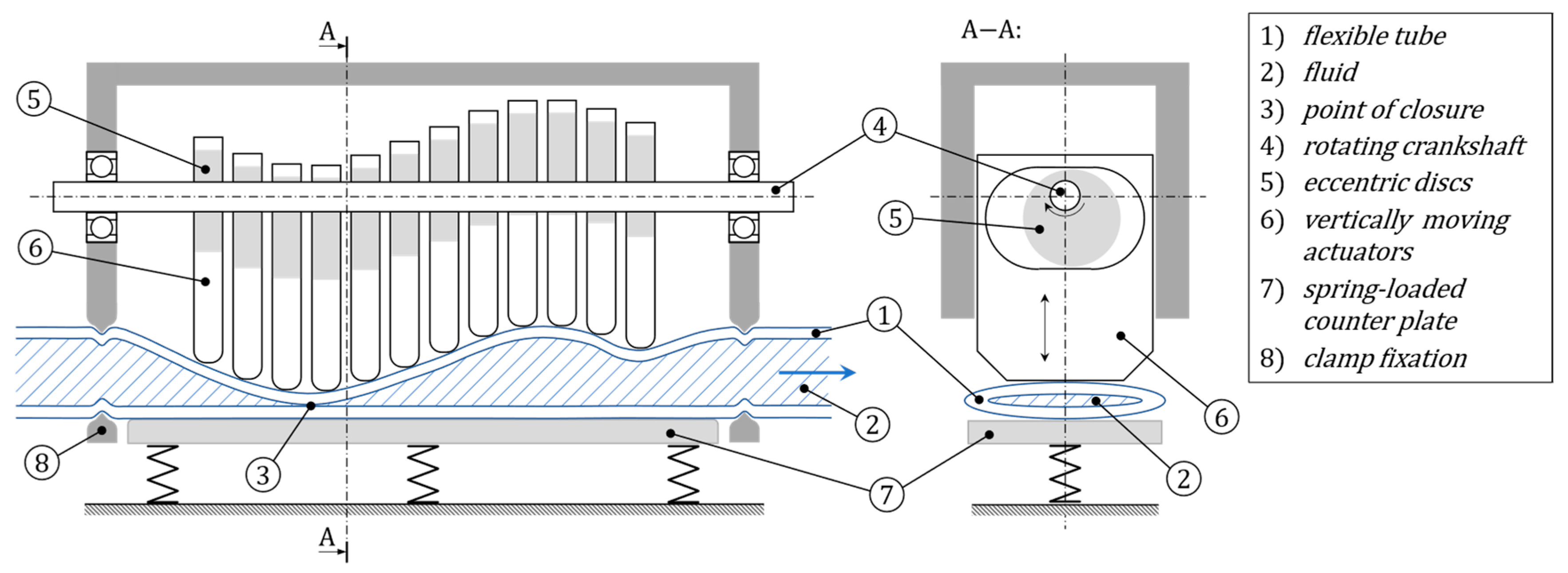
Peristaltic pumps are defined as (partly) flexible, silent, and fairly simple systems (Esser et al. (2019) [3]). They consist of a flexible member (hollow organs in nature or tubes in engineering), which is compressed by a force to (in most cases) fully close the inner conduit, resulting in a closed-off compartment being formed by the touching walls. The closure points or contractions are driven down the conduit via muscle contractions (nature) or actuators (e.g., rollers, pistons, or pneumatic chambers in engineering) in the direction of pumping (e.g., see Figure 1).
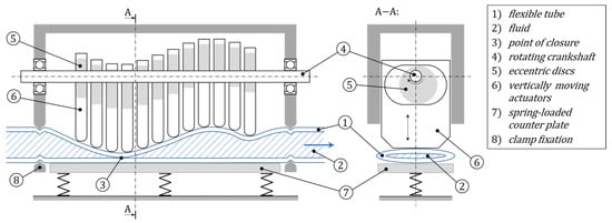
Figure 1.
Cross-sectional views of an exemplary peristaltic pump with a horizontal arrangement of vertically moving actuators. A flexible tube is pressed against the actuators by a spring-loaded counter plate and prevented from planar displacement by clamps. The cyclic movement of the actuators moves the point of closure of the tube and thus conveys the liquid.
While Panday et al. (2021) [4] investigated sloshing phenomena associated with wave-type excitation of the peristaltic conduit, such effects can be excluded from the hereby study. According to them, such phenomena only occur for wavelengths in and above the order of magnitude of the conduit opening.
1.2. General Setup for Current Study
For the current study, a simple hydraulic setup consisting of a peristaltic pump and two hydraulic subsystems (upstream and downstream of the pump, see Figure 2) was considered. The hydraulic subsystems feature generalized, independent, resistive and/or capacitive characteristics, and may each consist of an arbitrarily chosen selection of hydraulic elements. Flow rates within the upstream subsystem and downstream subsystem are obviously linked due to continuity, but do not necessarily correspond 1:1 because of the capacitive property of the fluid compartment within the pump.
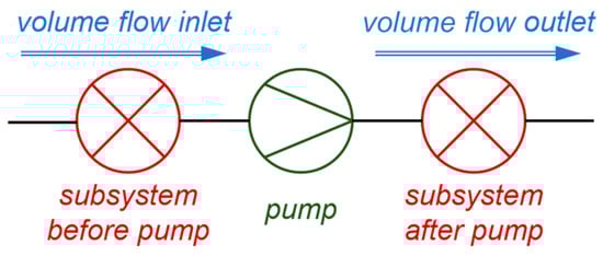
Figure 2.
Simplified hydraulic pump system overview. Separation between hydraulic subsystem before pump, peristaltic pump, and hydraulic subsystem after pump.
Although rotational pump designs are more common in industry, a linear design was chosen for this work to keep the simulation modelling simple. Other than rotary peristaltic pumps, this design has a set of translating actuators, which cyclically compress a conduit (i.e., a tube) in order to convey an enclosed liquid volume (see Figure 1 and Figure 3) by volumetric displacement. Clamps at the inlet and outlet of the pump hold the tube in position.
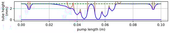
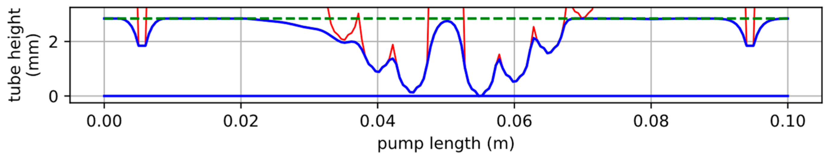
Figure 3.
Sectional view through the pump. The tube (thick blue lines) is axially fixed with clamps (thin red lines, left and right) and deformed by the peristaltic actuators (thin red lines, center). The undeformed tube is shown as a green, dashed line.
The pump design leads to the idealized assumption that the encapsulated liquid volume is constant with respect to pump frequency. Therefore, the expected flow rate is inversely proportional to the pump cycle time , as stated in the following Equation (1):
1.3. Problem Definition
The use of peristaltic pumps in a broader range of applications can present challenges. One such challenge concerns the appropriate selection of tubes in order to optimize operation.
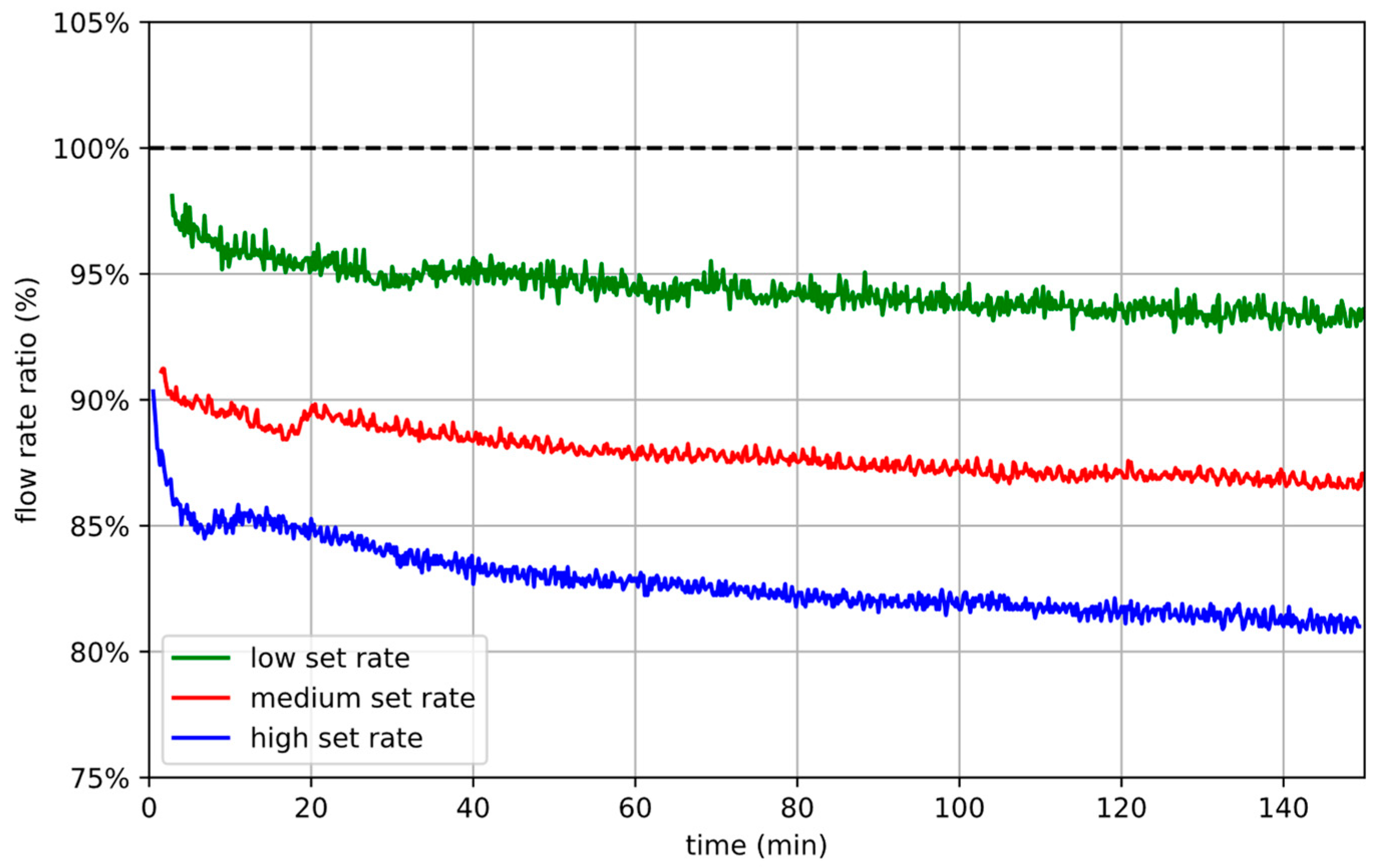
In certain cases, when peristaltic pumps are operated with polymer-based tube materials, the effective flow rate is often reported to be lower than the expected flow rate (see Figure 4). This reduction in pump performance can be characterized by the flow rate ratio, which is the ratio of effective-to-expected flow rate. At higher pumping frequencies, the elastic behavior of the tubing may show latency in keeping up with the position of the peristaltic actuators, resulting in a lift-off of the actuators and a reduction in the expected delivery volume. Also, the use of a more viscous tube material or a low inlet pressure can lead to lift-off effects and, thus, to reduced flow rate ratios. In addition, fatigue effects of the tube material often cause a gradual decrease in the flow rate ratio over time. Due to the complex interplay between these effects, the flow rate ratio is heavily dependent on the tube geometry, tube material, and operating conditions.

Figure 4.
Exemplary course of decreasing flow rate ratios for different pump rates over time. Low (green), medium (red), and high (blue) set rates show increasing dynamic losses. The fatigue effect of the tube material shows as an additional performance deterioration over time. The displayed data has been measured using the measurement setup Reference System described in Section 3.2, with cycle times of 8 s for the low, 2 s for the medium, and 1 s for the high flow rate.
To compensate for these effects, a prior set rate correction of the pump frequency can be considered. However, the determination of such corrections requires extensive and specific calibration measurements. This work focuses on providing a viable, less resource-intensive alternative to experimental calibration in terms of numerical simulation.
1.4. Numerical Modelling of Peristaltic Pumps
A series of numerical models of the peristaltic pumping process have been established in the context of biomedical as well as medical technology applications. These models are as follows.
Formato et al. (2019) [5] coupled hyper-elastic material dynamics and turbulence flow dynamics in order to describe the relevant physics of the peristaltic pumping process. In this context, the commercial finite element software ABAQUS 6.14 was used to investigate the performance of a representative peristaltic pump with a 3D transient model.
Yazdanpanah-Ardakani and Niroomand-Oscuii (2013) [6] presented a numerical investigation, which simulated a transient peristaltic transport by developing a model based on the fluid–solid interaction (FSI) method. In this work, the propagating wave through the conduit in which peristaltic flow occurred, was simulated by prescribing a set of displacements, along the radial direction, on the wall. Due to large deformations, they considered an adaptive discretization technique. Furthermore, they applied ADINA 8.5 as a finite element analytical software to study peristaltic transport. The results indicated that the presented numerical method could properly introduce the features of the flow.
Elabbasi et al. (2011) [7] applied COMSOL multiphysics to investigate the performance of a 180-degree rotary peristaltic pump with two metallic rollers and an elastomeric tube pumping a viscous Newtonian fluid. This work strongly coupled the deformation of the tube and the pumped fluid in terms of a FSI scheme. Hence, the implemented model captured the peristaltic flow, the flow fluctuations that result when the rollers engage and disengage the tube, and the contact interaction between the rollers and the tube. Consequently, Elabbasi et al. (2011) [7] described the usage of their combined finite element model to investigate the effect of pump design variations, such as tube occlusion, tube diameter, and roller speed, on the flow rate, flow fluctuations, and stress state in the tube.
Hung et al. (2015) [8] explored a numerical model to investigate the impact of changing the dimension of a soft tube in a peristaltic pump on deformation, stress, and fluid flow rate. The authors described the use of the commercial ANSYS software to calculate the deformation, stress, and fluid flow rate of the peristaltic pump in question.
Summarizing existing modelling attempts of the peristaltic pumping principle, the following can be stated.
Fully transient, finite element-based 3D structure mechanics simulations can provide insight into the dynamic tube deformation process within the peristalsis (see [5,6,7,8]). Furthermore, Yazdanpanah-Ardakani and Nirooomand-Oscuii (2013) [6] and Elabbasi et al. (2011) [7] have shown that a combination with FSI modelling approaches can predict the resulting fluid motion with sufficient accuracy. Herein, the term sufficient accuracy refers to the applicability of the presented models within practically relevant simulation-based product development schemes.
However, while potentially highly accurate, a full 3D dynamic FSI modelling approach is computationally very expensive. In order to effectively replace the above-mentioned experimental calibration procedure, hundreds of simulations, each covering relatively long timeframes, must be conducted. The process parameter space in question is particularly large since it needs to cover (i) the considered time of operation, (ii) range of pump rates, and (iii) relevant system operating conditions, as well as (iv) boundary conditions. With today’s cloud computing resources, conducting large sets of simulations in parallel has become feasible. Nevertheless, the temporal dimension of the process remains unsuited for distribution across multiple cores, and, therefore, constitutes a constraining factor. This limitation becomes particularly pronounced when addressing material fatigue, as a profound understanding of the behavior over extended periods encompassing tens of thousands of pump cycles becomes indispensable.
In order to present an industrially applicable numerical solution for pump calibration, the current work, therefore, drastically simplifies a full 3D transient FSI modelling approach towards a simple, fast, yet still sufficiently accurate 1D peristaltic pump solver.
1.5. The 1D Peristaltic Pump Solver
In the present work, a lean and fast multiphysics solver is presented as a numerical simulation-based alternative to the experimental calibration procedure. It uses a simplified 1D tube model to describe the relevant structural mechanics, volume displacement enforced by operational boundary conditions of the pump, as well as a 1D approach to model fluid dynamics. This ensures efficient generation of simulation results at low computational costs as well as sufficient accuracy.
The required simulation input parameters for the 1D peristaltic pump solver are as follows:
- Experimentally derived material properties (describing viscoelastic behavior, fatigue, stiffness, and pressure sensitivity).
- Hydraulic characteristics of the upstream- and downstream subsystems.
- Frequency of the pump cycle.
2. Methodology
2.1. Physics and Logic behind the 1D Peristaltic Pump Solver
The 1D peristaltic pump solver represents the deformed shape of the tube assuming that (i) the circumference of the tube remains constant regardless of its deformation state and that (ii) its deformed shape can be described by two horizontal, parallel plates connected by two half-pipes (as depicted in Figure 5). On this basis, the cross-sectional area of the tube at each position along its axis can be calculated in dependency of the local height and the undeformed tube diameter , as seen in the following Equation (2):
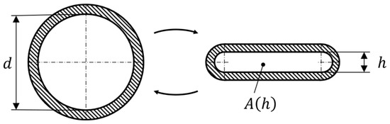
Figure 5.
Cross-section of the tube with undeformed (left) and deformed (right) shape as represented within the 1D peristaltic pump solver.
This amounts to a simple, one-dimensional description of the tube.
During the operation of the pump, the peristaltic actuators dynamically deform the tube, as depicted in Figure 1. During inwards motion, the actuator is in contact with the tube and the local height of the tube is, therefore, exclusively determined by the position of that actuator. During outward motion, on the other hand, a possible lift-off of the actuator must be considered.
In order to describe this process, a viscoelastic model is used. The tube is spatially discretized along and each slice is modelled as a spring-damper element, as depicted in Figure 6.
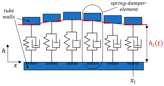
Figure 6.
Schematic sectional view of the tube inside the pump. The tube is discretized into segments, which are modelled as spring-damper elements.
Thus, the dynamic behavior of the height of the tube can be described as a harmonic oscillator according to the following Equation (3) (compare, e.g., Hayek (2003) [9]):
where and are coefficients describing elastic and viscous forces, respectively. Furthermore, the coefficient links the pressure difference between the tube and environmental pressures to the oscillation. The factor acts as a bending stiffness and compensates for bulges in the tube. By introducing the time-dependent factor as the equilibrium height (replacing the static tube diameter), it is possible to include time-dependent material fatigue effects in the modelling.
The hyperbolic nature of the differential Equation (3) used to describe local tube height inherently leads to the consideration of certain phenomena, like wave-type displacement along the tube or tube inertia in the context of dynamic tube deformation.
A key aspect in terms of the boundary conditions of the presented model is the assumption that the peristaltic actuators lock tightly. Since the general pump functionality relies on the fact that always exactly one actuator locks the flow, the fluid volume within the tube is effectively divided into two hydraulically separated capacities: the upstream- and downstream subsystems ( upstream- and downstream of the closure, as depicted in Figure 2 and Figure 7). Thus, the flow rates within the two subsystems ( and ) are independently enforced by geometric constraints (=volume replacement due to actuator motion) as seen in Equation (4).
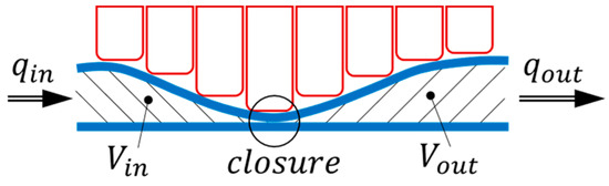
Figure 7.
Schematic sectional view of the actuators compressing the tube. The fluid domain is separated into upstream (“in”) and a downstream (“out”) parts by the point of closure forced by the actuators.
In the context of Equation (4) and can be calculated from the integration of Equation (2) along .
Using a momentum balance, the rate of change in the fluid flow rate can be put in relation to the forces acting on each tube segment, as follows:
In Figure 8, the corresponding scenario is depicted. The length and cross-section of the tube segment are denoted with and , respectively, and the fluid density is . The geodetic height between the inlet and outlet of the segment is denoted with and the corresponding pressures are and . The difference in geodetic height within any given tube segment is usually a known process parameter. The flow rate-dependent pressure loss must be determined experimentally. All losses, such as friction, turbulence, or losses due to radial or azimuthal velocity components are included in this parameter. The rate of change in the flow rate is enforced by the pump according to Equation (4). Consequently, the pressure difference p1-p2 within any given tube segment (e.g., subsystem) can be derived as remaining unknown using Equation (5).
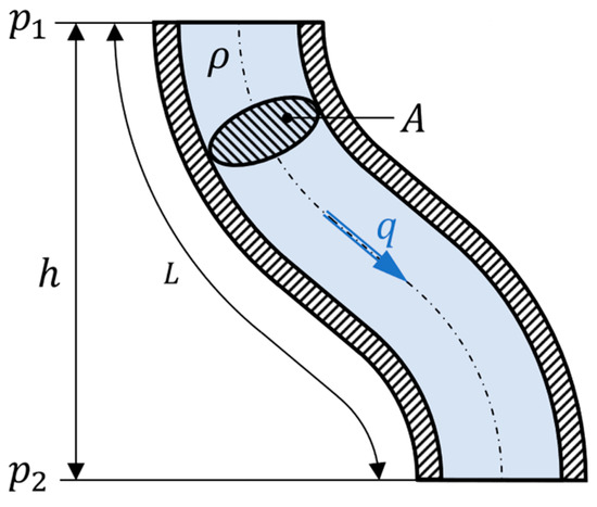
Figure 8.
Cross-section through a generalized tube-segment.
Since this logic holds for any number of consecutive tube segments, it can be used to expand any tube segment to either one of the two downstream/upstream subsystems within Figure 2.
2.2. Experimental Determination of Material Properties
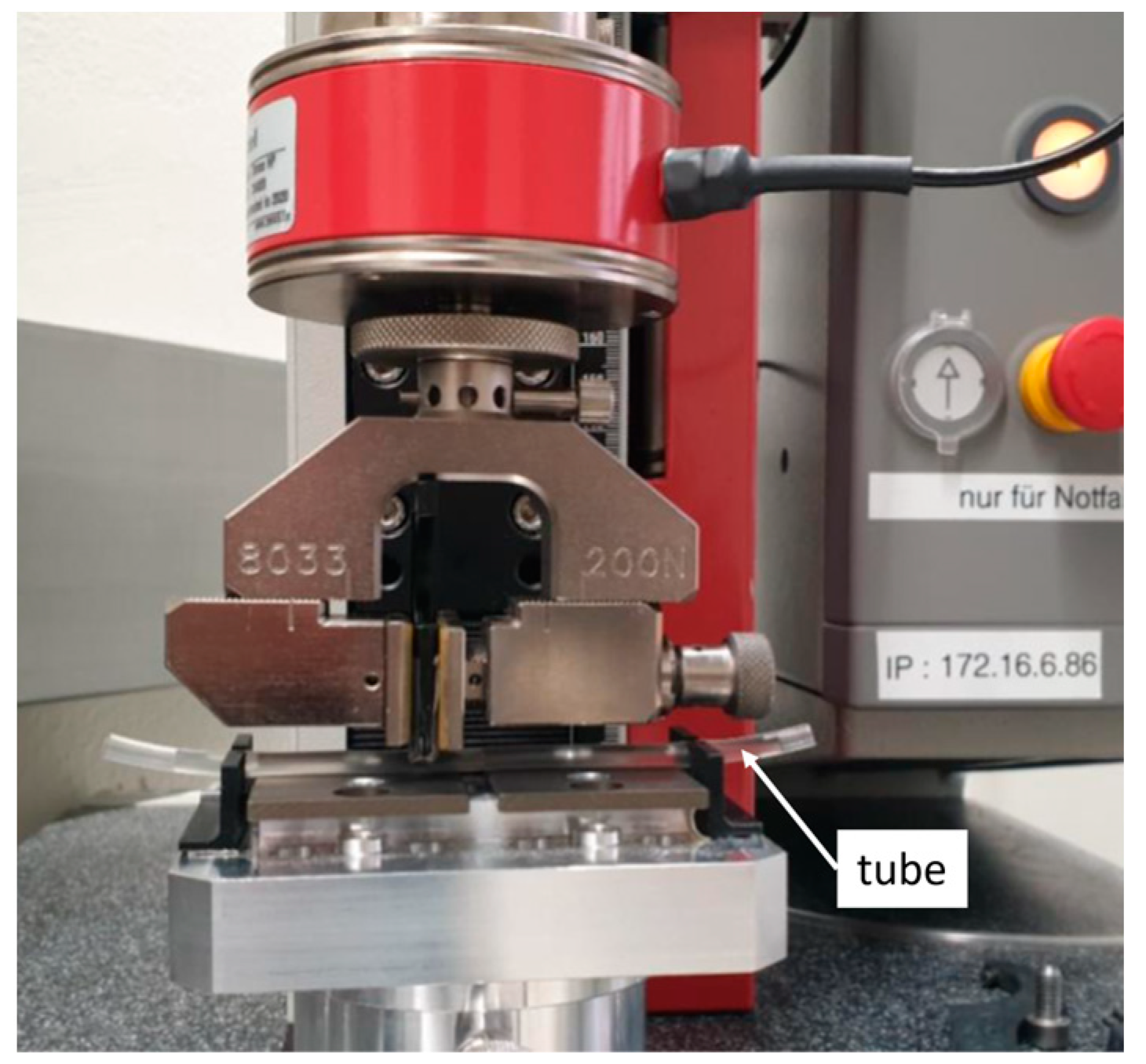
To provide the material properties, which represent elastic and viscous force effects used in Equation (3) (the coefficients and , respectively), mechanical measurements were conducted. An industrial tension compression testing apparatus (see Figure 9) was used to analyze the elastic behavior of each considered tube material during deformation by a peristaltic actuator. The damping coefficients were identified by dynamic deformation measurements at varying deformation speeds on this apparatus.

Figure 9.
Industrial tension compression testing apparatus for the determination of the elastic and viscous tube material properties.
In terms of determination of the equilibrium height , the scaling of the tube diameter with a logarithmic decay function, as shown in the following Equation (6), was found to model the fatigue effect quite well:
Model parameters and were derived by curve fitting the results of long-term flow measurements at low pump rates (850 s per pump cycle) with Equation (6), as shown in Figure 10. For curve fitting of the flow measurements, the scale factor is also initially treated as a curve fitting parameter. In order to use the found decay function to describe the equilibrium height, the scale factor must again be replaced by the tube diameter . The flow measurements were carried out for each considered material in analogy to the Reference System setup described in Section 3.2.
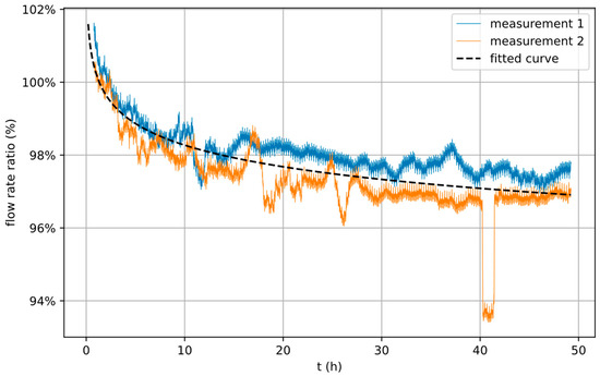
Figure 10.
Measured flow rates (blue, orange) and fitted curve (dashed, based on Equation (6)) over time. The shape of the fitted curve is used to model the fatigue effect of a specific tube material.
The remaining unknown constants and from Equation (3) were iteratively narrowed down by visually comparing simulation results based on estimated values for and with flow measurements and then stepwise adjusting the values. In contrast to parameters and , these parameters showed no discernible dependence on the tube material used. They were, therefore, assumed to be constant model parameters.
2.3. Implementation of the 1D Peristaltic Pump Solver
The 1D peristaltic pump solver was implemented using the programming language Python3 (Van Rossum and Drake (2009) [10]). This choice represents a trade-off between developer-friendliness and efficiency. To improve the performance, the open-source packages Numba and NumPy were used (see Lam et al. (2015) [11] and Harris et al. (2020) [12]).
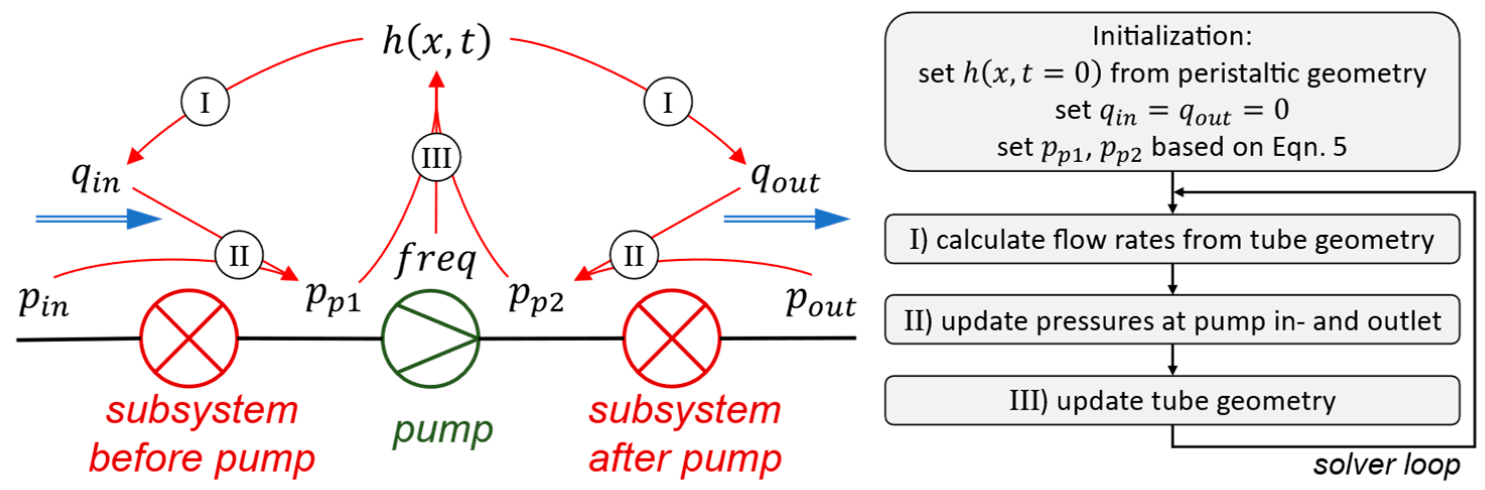
The schematic workflow of the 1D peristaltic pump solver is depicted in Figure 11 and plays out as follows:
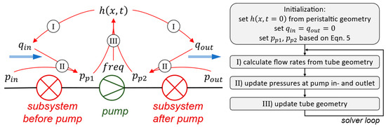
Figure 11.
Schematic workflow of the 1D peristaltic pump solver.
- (I)
- The inlet and outlet flow rates and as well as their rates of change follow from the geometric constraints of the tube geometry (Equations (2) and (4))
- (II)
- The pump inlet and outlet pressures and can then be calculated via Equation (5), applied to both subsystems. Therefore, the rate of change in the flow rates over the corresponding subsystem as well as appropriate system boundary conditions need to be inserted. The boundary conditions are determined by system parameters, namely:
- Inlet and outlet pressures, and (e.g., both equal to the environmental pressure).
- Difference in geodetic height within subsystems.
- Pressure loss function for the respective subsystem.
- (III)
- The tube height is then updated for the next time step, taking into account the outward motion of the actuators and the material-dependent spring-damping properties of the tube via Equation (3).
For stability reasons, an implicit method was used to numerically solve the second order differential Equation (7) for the tube height. The used trapezoidal method according to, e.g., Burden and Faires (2000) [13] yields the following:
where is introduced as a new variable to transform the second order differential equation for the tube height to a system of first order differential equations (see Burden and Faires (2000) [13] and Atkinson (1989) [14]), where denotes the time step.
3. Results
3.1. Validation Procedure
To validate the 1D peristaltic pump solver, comparisons were made between flow rate measurements of different subsystem setups and the results of the corresponding numerical simulations. To test the frequency dependence of the process, three different pump rates were considered, as follows:
- High pump rate with of 0.8 s.
- Medium pump rate with of 4 s.
- Low pump rate with of 32 s.
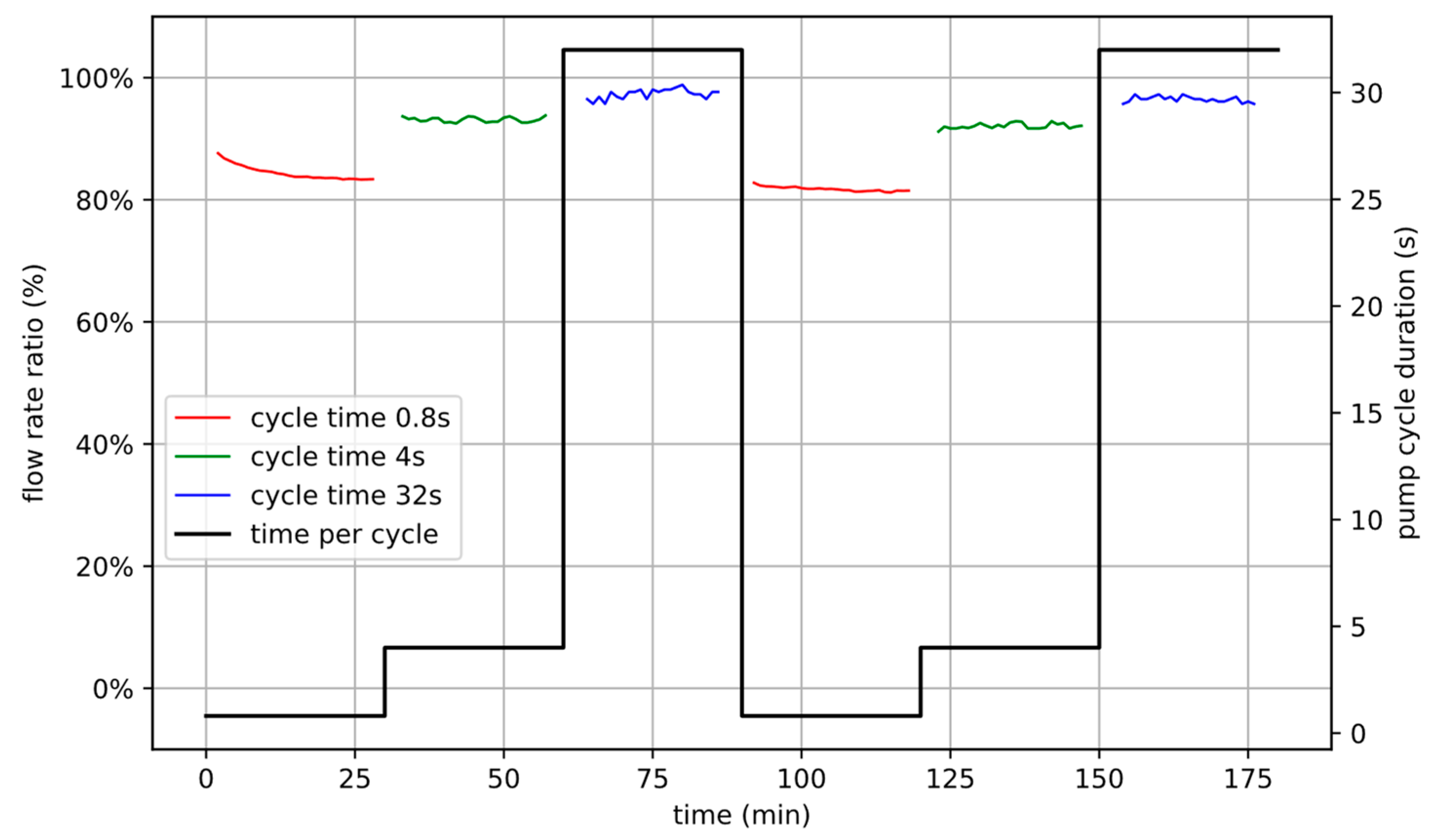
Each of these pump rates has been applied for 30 min. The experiments were conducted as consecutive phases within a single prolonged experimental workflow, to minimize other influences, like (i) differences in clamping of the tube and (ii) variations in diameter or (iii) material properties between different tube sections. To gain a more precise understanding of the fatigue behavior of the material during extended operational periods, the sequence was repeated a second time on the same setup. In the following, we refer to the first three phases as (I) and to the repetitions as (II).
The resulting six experimental phases are shown in Figure 12. The measured flow rates of each phase were scaled by the expected flow rate of the corresponding pump setting and plotted as percentages of the expected flow rate (flow rate ratio) over time.
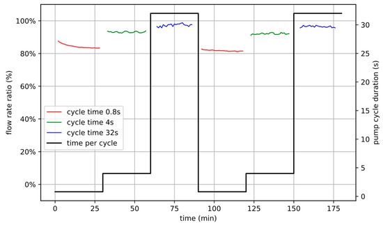
Figure 12.
Measurement protocol of the validation measurements as a function of time. Each measurement consists of six sequential phases (thick line), 30 min each, with a high pump rate (), a medium pump rate (), and a low pump rate (), repeated twice. Exemplary flow rate ratios of such a measurement are plotted as red, green, and blue thin lines for of 0.8 s, 4 s, and 32 s, respectively.
3.2. Measurement Setup
To conduct the flow measurements, the following setup was used. The peristaltic pump (see Figure 13) was utilized to pump water from a supply tank into a collection tank (see Figure 14, top). The collection tank was positioned on a scale, enabling the measurement of the amount of liquid pumped through per unit of time. With an absolute measurement precision of of the scale and a delivery volume of per pump cycle, as specified by the pump manufacturer, the experimental accuracy in terms of flow rate ratio can be calculated for each individual pump rate. This leads to a measurement precision of +/−0.06% for the high pump rate, +/−0.3% for the medium pump rate, and +/−2.3% for the low pump rate.
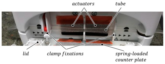
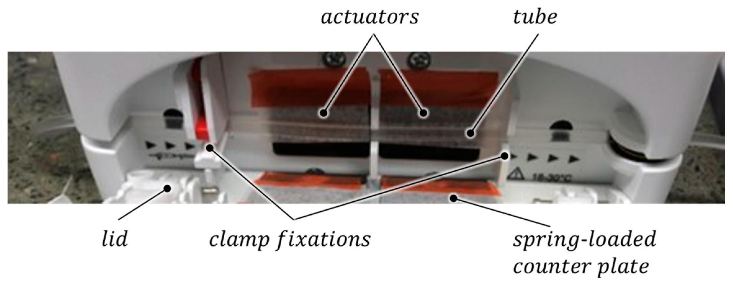
Figure 13.
Photo of the experimental setup. The image shows the peristaltic pump with horizontally inserted tube and opened lid. Two sets of six actuators each are located behind the tube (hidden by a protective foil). The tube is prevented from slipping with clamps. The lid contains a spring-loaded counter plate that presses the tube against the actuators (in the closed state).
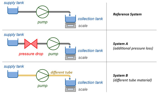
Figure 14.
Schematic illustration of the measurement setups used in the validation. The peristaltic pump was used to pump a liquid from a supply tank through individual tube systems into a collection tank. The collection tank is positioned on a scale, enabling the measurement of the amount of pumped liquid. In the Reference System (top), the setup involves only pump, supply tank, tube, collection tank, and scale. In System A (middle), an additional pressure drop component has been added upstream of the pump. In System B (bottom), a different tube material was used.
To test the different aspects of the process, one reference setup (Reference System) and two other setups with varying hydraulic properties were measured, as follows (see Figure 14):
System A: Additional pressure loss element upstream of the pump inlet as compared to the Reference System (about 40 times higher pressure loss).
System B: Same setup as the Reference System but with a different tube material.
3.3. Qualitative Results
In Figure 15, Figure 16 and Figure 17, the measured results of the flow-experiments and the corresponding numerical predictions, as derived from the 1D peristaltic pump solver, are plotted for cycle times of 0.8 s, 4 s, and 32 s, respectively.
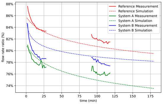
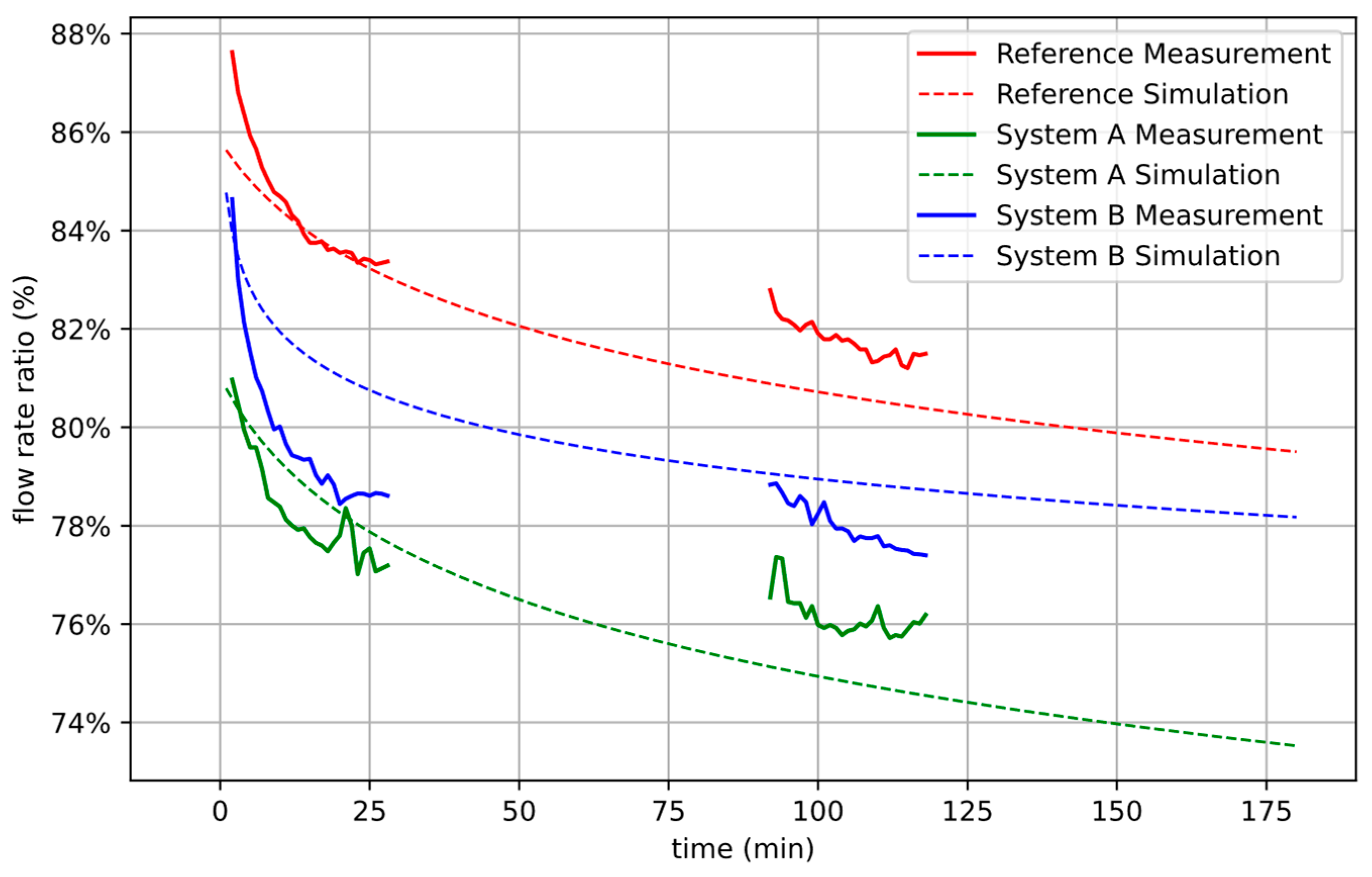
Figure 15.
Comparison between simulated (dashed line) and measured flow rate ratios (solid line) for short cycle time of 0.8 s (=high flow rates) and Reference System (red), System A (green) and System B (blue). The accuracy of the measurement is +/−0.06% in terms of flow rate ratio.
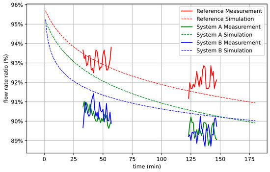
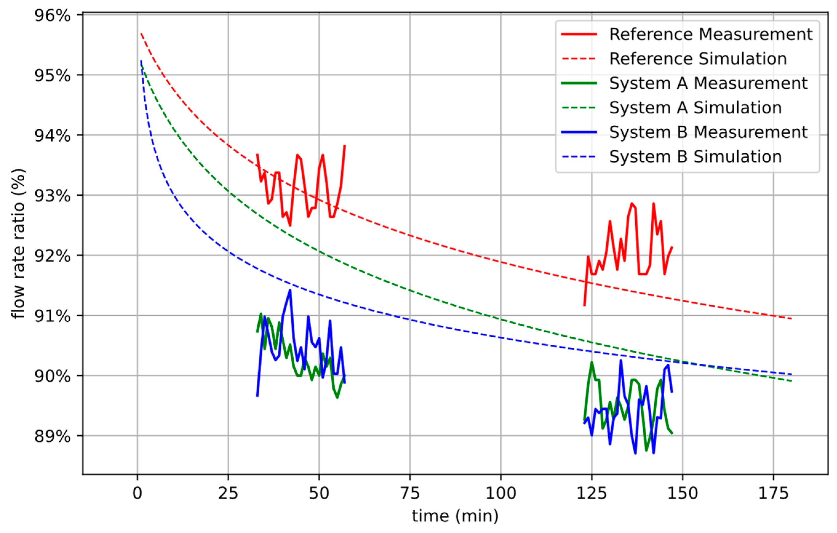
Figure 16.
Comparison between simulated (dashed line) and measured flow rate ratios (solid line) for the medium cycle time of 4 s (medium flow rate) and Reference System (red), System A (green), and System B (blue). The accuracy of the measurement data is +/−1.5% in terms of flow rate ratio.

Figure 17.
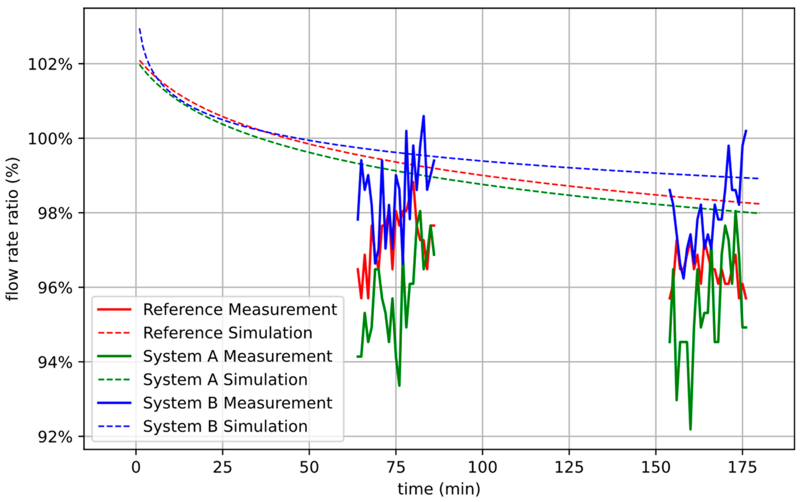
Comparison between simulated (dashed line) and measured flow rate ratio (solid line) for a long cycle time of 32 s (low flow rates) and Reference System (red), System A (green), and System B (blue). The accuracy of the measurement data is +/−2.3% in terms of flow rate ratio.
In Figure 15, the results of the three system setups are plotted for the high flow rates retrieved during the first and fourth phase of the experimental workflow according to Figure 12. At these high flow rates, the larger pressure loss upstream of the pump inlet within System A has a significant negative effect on the measured flow rate ratios. It can be seen that the alternative tube material of System B also performs significantly worse than that of the Reference System. The simulation qualitatively predicts these trends.
Figure 16 shows the results of the three system setups for the medium flow rates retrieved during the second and fifth phase of the experimental workflow according to Figure 12. At these medium flow rates, System A and System B both perform worse than the Reference System. While the simulation correctly predicts this qualitative trend, the distinction between System A and System B is predicted to be somewhat greater than indicated by the measurements. However, the observed differences and similarities lie within the order of magnitude of deviations due to the limits of experimental accuracy.
The results of the three system setups for the low flow rates retrieved during the third and sixth phase of the experimental workflow according to Figure 12 are plotted in Figure 17. At these low flow rates, System B shows less performance decline than the other two systems. This may indicate a lower viscosity to elasticity ratio in this material compared to that of the reference material (used in Reference System and System A). It can also be seen that the fatigue effect of the reference material is greater. The simulation predicts this behavior to be qualitatively correct.
3.4. Quantitative Results
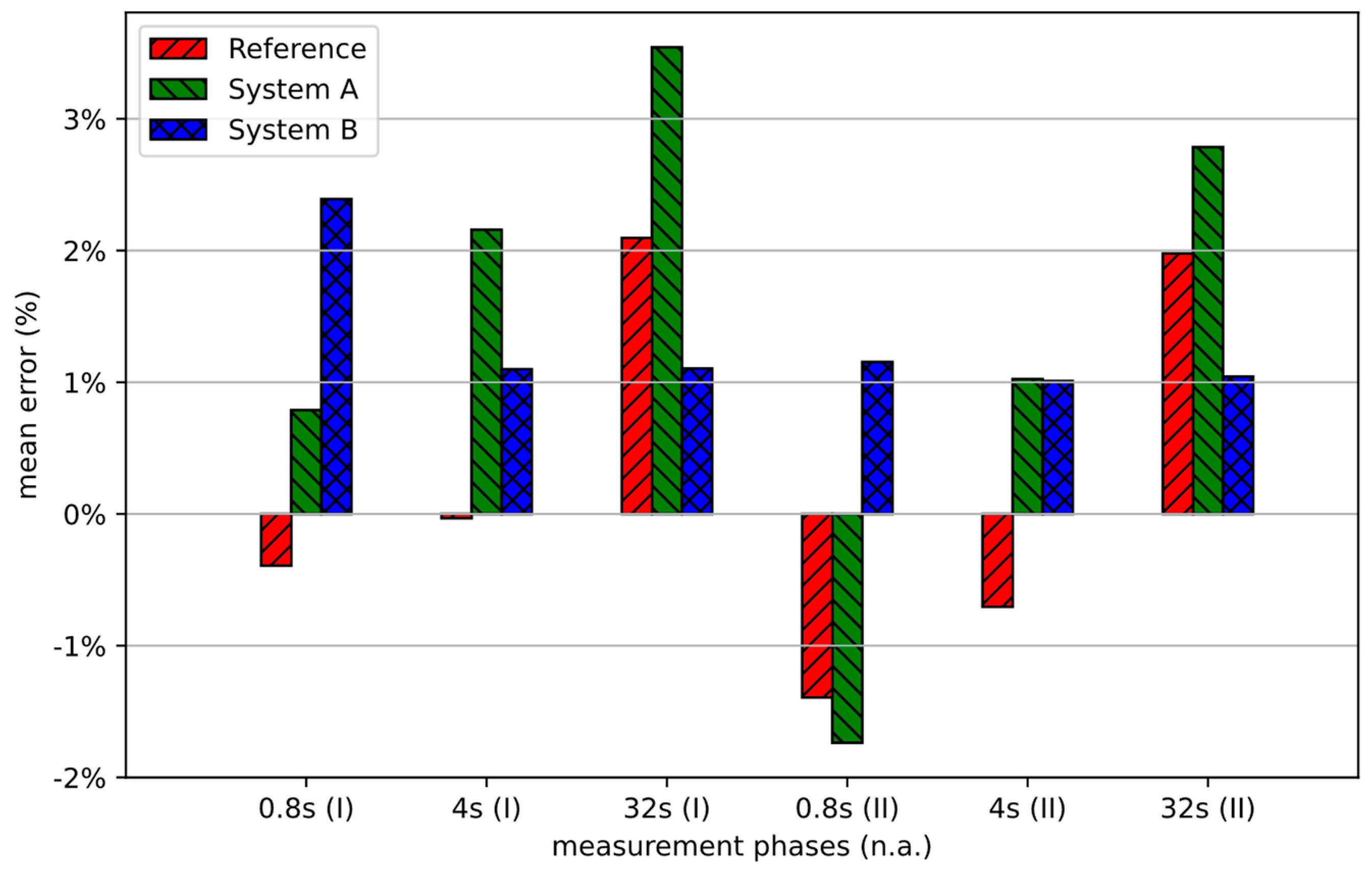
In Figure 18, the deviations between the simulation and the measurements are shown for each of the six phases of the experimental workflow according to Figure 12. Each bar represents a time-average over the whole corresponding phase.
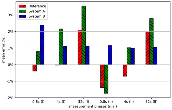
Figure 18.
Time-averaged deviations between simulated and measured flow rate ratios for each of the six experimental phases, according to Figure 12.
A comparison of the time-averaged deviations between the simulated and measured results shown in Figure 18 yields several conclusions, as follows:
- Overall Accuracy: The largest observed relative deviation amounts to −3.5% (phase 32 s(I), System A), compared to an estimated accuracy of measurements of +/−2.3%. This speaks for the high degree of overall accuracy of the applied predictive method as well as for the general validity of the scheme. The presented investigations cover a wide parameter window, as follows:
- Three different pump rates (indicated as 0.8 s, 4 s, and 32 s cycle times).
- Three different hydraulic subsystem setups (Reference System, System A, and System B).
- Two material types (reference material: Reference System and System A vs. alternative material: System B).
- Material fatigue effects at different operating times (initial vs. latter experimental phases, indicated as (I) and (II), respectively).
- Impact of Pump Rate: As a general tendency, the solver appears to show a positive result deviation correlation to the applied pump cycle time. While no clear over- or underestimation of the flow rate ratio occurs with low cycle times (see phases with a cycle time of 0.8), a more pronounced overestimation of the flow rate ratios becomes apparent with increasing cycle times (see phases with a cycle time of 32 s).
- Impact of Fatigue Effect: The tube material fatigue effect can best be observed by comparing experimental phases 0.8 s(I) vs. 0.8 s(II), 4 s(I) vs. 4 s(II), and 32 s(I) vs. 32 s(II). As a general tendency, the solver appears to show a slight positive deviation correlation to progressing fatigue. The longer the actual tube material is exposed to application conditions, the smaller the underestimation and the higher the overestimation of the flow rate ratios becomes.
- Material Effect: As a general tendency, the described impact of both pump rate and fatigue effect on solver accuracy appears somewhat more pronounced for the model of the reference material (Reference System and System A) than for the model of the alternative tube material (System B). However, general qualitative tendencies correspond for both material model types.
4. Conclusions and Outlook
The presented fast 1D peristaltic pump solver was shown to reproduce all relevant process- as well as material-related effects affecting peristaltic pump flow rate. It achieves qualitatively satisfying as well as quantitatively satisfying results. The arbitrarily high precision of elaborate 3D FSI simulations may not be reproduced, but it might be justifiable for industry purposes. A big advantage of the presented solver is that only one single flow measurement, along with few tension–compression tests, are required per tube material in order to retrieve the material parameters necessary to run the solver. Thus, the presented simulation-based calibration procedure greatly simplifies the conventional calibration process. This enables the application of peristaltic pumps in previously unexplored fields.
Future improvements in the 1D peristaltic pump solver could include a deeper study of fatigue effects in order to omit the still required flow measurement. Accuracy could be further increased by including analytical or empirical models for the material parameters and in Equation (3), which might be connected to geometrical properties of the tube and the viscoelastic material properties and . Furthermore, it would be of interest to investigate a rotary pump design, which is more commonly prevalent in the industry.
Author Contributions
Conceptualization, R.G. and R.M.F.; methodology, M.H., S.S. and F.D.L.; software, M.H.; validation, M.H. and R.G.; formal analysis, M.H. and R.G.; investigation, R.G., C.J. and S.K.; resources, R.G., C.J., S.K. and G.K.B.; data curation, R.G. and C.J.; writing—original draft preparation, M.H. and G.K.B.; writing—review and editing, M.H., R.G., S.S., F.D.L., R.M.F., D.W. and G.K.B.; visualization, M.H. and R.G.; supervision, R.M.F. and G.K.B.; project administration, R.M.F.; funding acquisition, R.M.F. All authors have read and agreed to the published version of the manuscript.
Funding
This research was funded by Innosuisse—Swiss Innovation Agency (no. 34150.1 IP-ENG).
Data Availability Statement
The data that support the findings of this study are available from the corresponding author upon reasonable request.
Conflicts of Interest
The authors declare no conflict of interest. The funders had no role in the design of the study; in the collection, analyses, or interpretation of data; in the writing of the manuscript; or in the decision to publish the results.
Nomenclature
| Expected flow rate in | |
| Duration of one pump cycle in | |
| Encapsulated liquid volume in the peristalsis in | |
| Time in | |
| Coordinate along the axis of the tube in | |
| Cross-sectional area of the tube in | |
| Diameter of the tube in | |
| Height of the (deformed) tube in | |
| Density of the liquid in | |
| Length of a tube segment | |
| Coefficient for the elastic behavior of the tube in | |
| Coefficient for the viscous behavior of the tube in | |
| Coefficient for the pressure dependency of the tube in | |
| Coefficient for the stiffness of the tube in | |
| Pressure in the tube in | |
| Environment pressure in | |
| Desired height of the tube considering the material-fatigue in | |
| Flow rate upstream of the pump in | |
| Flow rate downstream of the pump in | |
| Liquid volume upstream of the closure in the pump in | |
| Liquid volume upstream of the closure in the pump in | |
| Pressure at the inlet of a generalized tube segment in | |
| Pressure at the outlet of a generalized tube segment in | |
| Pressure loss over a generalized tube segment in | |
| Pressure at the inlet of the pump in | |
| Pressure at the outlet of the pump in | |
| Model parameters for curve fitting of the equilibrium height | |
| Variable used to transform the second order differential equation for the tube height into matrix form | |
| Gravity of Earth in |
References
- Klespitz, J.; Levente, K. Peristaltic pumps—A review on working and control possibilities. In Proceedings of the IEEE 12th International Symposium on Applied Machine Intelligence and Informatics (SAMI), Herl’any, Slovakia, 23–25 January 2014; pp. 191–194. [Google Scholar]
- Berg, J.; Dallas, T. Peristaltic Pumps. In Encyclopedia of Microfluidics and Nanofluidics; Li, D., Ed.; Springer: Boston, MA, USA, 2008. [Google Scholar] [CrossRef]
- Esser, F.; Masselter, T.; Speck, T. Silent Pumpers: A Comparative Topical Overview of the Peristaltic Pumping Principle in Living Nature, Engineering, and Biomimetics. Adv. Intell. Syst. 2019, 1, 1900009. [Google Scholar] [CrossRef]
- Panday, S.; Floryan, J.M.; Faisal, K.M. On the peristaltic pumping. Phys. Fluids 2021, 33, 033609. [Google Scholar] [CrossRef]
- Formato, G.; Romano, R.; Formato, A.; Sorvari, J.; Koiranen, T.; Pellegrino, A.; Villecco, F. Fluid–Structure Interaction Modeling Applied to Peristaltic Pump Flow Simulations. Machines 2019, 7, 50. [Google Scholar] [CrossRef]
- Yazdanpanah-Ardakani, K.; Niroomand-Oscuii, H. New approach in modeling peristaltic transport of non-Newtonian fluid. J. Mech. Med. Biol. 2013, 13, 1350052. [Google Scholar] [CrossRef]
- Elabbasi, N.; Bergström, J.; Brown, S. Fluid-Structure Interaction Analysis of a Peristaltic Pump. In Proceedings of the COMSOL Conference, Boston, MA, USA, 13–15 October 2011. [Google Scholar]
- Hung, N.B.; Ock, T.L. The study about deformation of a Peristaltic Pump using Numerical Simulation. Korean Hydrog. New Energy Soc. 2015, 26, 652–658. [Google Scholar] [CrossRef]
- Hayek, S.I. Mechanical Vibration and Damping. In Encyclopedia of Applied Physics; WILEY-VCH Verlag GmbH & Co KGaA: Hoboken, NJ, USA, 2003; ISBN 9783527600434. [Google Scholar] [CrossRef]
- Van Rossum, G.; Drake, F.L. Python 3 Reference Manual; CreateSpace: Scotts Valley, CA, USA, 2009. [Google Scholar]
- Lam, S.K.; Pitrou, A.; Seibert, S. Numba: A LLVM-based Python JIT compiler. In Proceedings of the Second Workshop on the LLVM Compiler Infrastructure in HPC (LLVM ‘15), Austin, TX, USA, 15 November 2015; Association for Computing Machinery: New York, NY, USA, 2015; p. 7. [Google Scholar] [CrossRef]
- Harris, C.R.; Millman, K.J.; van der Walt, S.J.; Gommers, R.; Virtanen, P.; Cournapeau, D.; Wieser, E.; Taylor, J.; Berg, S.; Smith, N.J.; et al. Array programming with NumPy. Nature 2020, 585, 357–362. [Google Scholar] [CrossRef] [PubMed]
- Burden, R.L.; Faires, J.D. Numerical Analysis, 7th ed.; Brooks/Cole: Totnes, UK, 2000; ISBN 978-0-534-38216-2. [Google Scholar]
- Atkinson, K.E. An Introduction to Numerical Analysis, 2nd ed.; John Wiley & Sons: New York, NY, USA, 1989; ISBN 978-0-471-50023-0. [Google Scholar]


Disclaimer/Publisher’s Note: The statements, opinions and data contained in all publications are solely those of the individual author(s) and contributor(s) and not of MDPI and/or the editor(s). MDPI and/or the editor(s) disclaim responsibility for any injury to people or property resulting from any ideas, methods, instructions or products referred to in the content. |
© 2023 by the authors. Licensee MDPI, Basel, Switzerland. This article is an open access article distributed under the terms and conditions of the Creative Commons Attribution (CC BY) license (https://creativecommons.org/licenses/by/4.0/).