Improving Pump Characteristics through Double Curvature Impellers: Experimental Measurements and 3D CFD Analysis

Abstract

The outlet angle and shape of impeller blades are important parameters in centrifugal pump design. There is a lack of detailed studies related to double curvature impellers in centrifugal pumps in the current literature; therefore, an experimental and numerical analysis of double curvature impellers was performed. Six impellers were made and then assessed in a centrifugal pump test bed and simulated via 3D CFD simulation. The original impeller was also tested and simulated. One of the manufactured impellers had the same design as the original, and the other five impellers had a double curvature. Laboratory tests and simulations were conducted with three rotation speeds: 1400, 1700, and 1900 RPM. Head and performance curve equations were obtained for the pump–engine unit based on the flow of each impeller for the three rotation speeds. The results showed that a double curvature impeller improved pump head by approximately 1 m for the range of the study and performance by about 2% when compared to basic impeller. On the other hand, it was observed that turbulence models such as k-ε and SST k-ω reproduced similar physical and numerical results.

1. Introduction

Fluid transportation is important and necessary, and the most-used mechanism for transportation is a centrifugal pump. Centrifugal pumps comprise several components required for adequate performance, two of which are the impeller and volute. The impeller’s geometry is critical because it adds energy to the fluid [1], whereas the volute converts kinetic energy to pressure energy. The impeller is the pump’s most important moving element [2]. The blade, which is a key component of the impeller, directs the flow as it passes through the impeller.

The relevant variables that affect flow through the interior of the centrifugal pump are as follows: rotational speed of the pump, number of impeller blades, impeller diameters (interior and exterior), pump head, and the fluid being pumped [3,4]. A kinematic study of the impeller is essential when analyzing the load that the pump can deliver, whereas some equations can be used to analyze the behavior of turbomachines, for example, the Euler equation based on head or Euler’s theoretical height, tangential velocities, and gravitational forces [2,3,4].

Advancements in computational technology, and, subsequently, computational fluid dynamics (CFD), have made the latter a frequently used tool for analyzing and designing fluid impelling machines. A CFD analysis typically consists of three phases: pre-processing, processing, and post-processing.

Several experimental and CFD studies have been carried out on centrifugal pumps, including studies on pressure pulsations using numerical methods [5]. Spence and Amaral [6] employed the Taguchi methodology to establish various configurations for analyzing the impact of several parameters on pressure pulsations. Instead of conducting a complete factorial analysis, which would have required 243 trials, the authors used the Taguchi methodology on an L9 matrix with 27 trials. The simulation was based on previously conducted experimental testing. Fontanals et al. [7] used CFD to investigate pressure fluctuations caused by the interaction between the pump’s impeller and diffuser and compared the results with experimental findings.

Several studies have carried out experimental analyses of centrifugal pump efficiency improvements based on impeller trim [8]. The radial load on a pump’s impeller working under off-design conditions was simulated and experimentally validated [9]. Other studies have investigated the influence of the number of blades [10,11,12,13,14], impeller inlet geometry [15,16,17], blade outlet angle in centrifugal pumps [18], and blade outlet geometry [19]. Patil et al. [20] conducted CFD analysis with various blade inlet angles and compared the results with experimental results. After obtaining better results through CFD, the authors concluded that the difference was due to the friction present in the experimental tests.

Two-dimensional simulations have been used to study flow through impellers and to determine performance, head, and efficiency curves using an optimization algorithm [21]. Grapsas et al. [22] conducted experimental and CFD studies in 2D. Zhou et al. [23] also studied flow through a centrifugal pump using CFD, but in 3D, under both normal design conditions and off-design conditions. Yang et al. [24] carried out 3D studies that simulated turbulent flows on the interior of a centrifugal pump for chemical products and compared the distribution of pressures and relative velocity under different work conditions. Shvindin and Ivanyushin [25] and Cheah et al. [26] studied the primary performance characteristics of a pump under off-design conditions. Barrio et al. [27] conducted CFD and 3D studies in the pumps’ near-tongue region based on previously developed experimental trials with flow velocities ranging from 20% to 160% of the nominal flow rate. Ozturk et al. [28] studied the effect of the impeller–diffuser separation on a centrifugal pump. Gupta et al. [29] carried out simulation studies to analyze the pressure and velocity distributions on impeller interiors.

Asuaje et al. [30] investigated the volute’s influence on pressure and velocity fields and highlighted that, despite good flow orientation in the volute, there is heavy recirculation at the volute’s outlet and uniformity in flow velocity in the spaces between the blades. Esfahani et al. [31] conducted studies with different numbers of blades [5,6,7,8] and modified the volute’s shape (circular and elliptical). Kulkarni [32] performed CFD studies and highlighted the importance of surface finish for a centrifugal pump’s efficiency as one of the significant conclusions.

There are numerical studies available on pumps that work with viscous fluids. Shojaeefard et al. [17,33,34] conducted experimental studies and simulations where they varied the impeller’s width and outlet angle while pumping water and oil. Pegalthivarthi et al. [35] utilized CFD to examine the effect of different operating conditions and geometries on pumping a dense slurry.

Experimental studies were conducted by Mustafa Gölcü and Pancar [36] on impellers with varying numbers of blades and different separator lengths. Baoling et al. [37] performed 3D simulations using impellers with different blade lengths (long, medium, and short) in various combinations, comparing the relative velocity and pressure distribution. Kaya and others [38] measured the efficiency of different pumps operating in an industrial plant to perform efficiency studies and provide recommendations for improvement.

Several investigations have demonstrated the significance of CFD in centrifugal pump design [39,40]. Additionally, CFD studies have been utilized to forecast or analyze the cavitation phenomenon in centrifugal pumps [41,42,43,44]. Shah et al. [45] emphasized the importance and usefulness of numerical simulations in current advances in centrifugal pumps and referenced studies conducted in this area.

Blades can be constructed in three ways based on the impeller outlet angle (${\beta }_2$): forward-curved (${\beta }_2$ > 90°), backward-curved (${\beta }_2$ < 90°), or radial (${\beta }_2$ = 90°). Impellers made with forward-curved blades generate more head than those with backward-curved blades, but they consume significantly more power. Therefore, impellers are usually produced with backward-curved blades [46]. Studying double curvature blades would be worthwhile to determine at what distance between the interior and exterior impeller diameters the double curvature can be applied to achieve a higher flow and head, thus preserving or improving the pump’s performance.

On the other hand, different CFD analyses have recently been conducted. Ke et al. (2023) [47] studied the pressure and velocity distribution in the inter-blade channel by installing a trimmed splitter blade. Using CFD, they determined the thickness, diameter, and length of the inter-blade for the pump used. Hu et al. (2023) [48] conducted CFD analysis on centrifugal pumps operating with drilling fluids, which are non-Newtonian fluids. They investigated the viscous effect caused highly irregular flow at the blade outlet.

There is a paucity of in-depth studies concerning impellers with double curvature blades in the current literature. As such, the aim of this study is to evaluate double curvature impellers at varying rotational speeds through experimental measurements and CFD models. The aim is to obtain the head and performance curves of the pump–engine unit for each impeller design at different flow rates. Lastly, the results obtained from the experimental and numerical simulation curves are compared, with the simulations showing better outcomes, primarily due to the friction present in the experimental results.

2. Materials and Methods

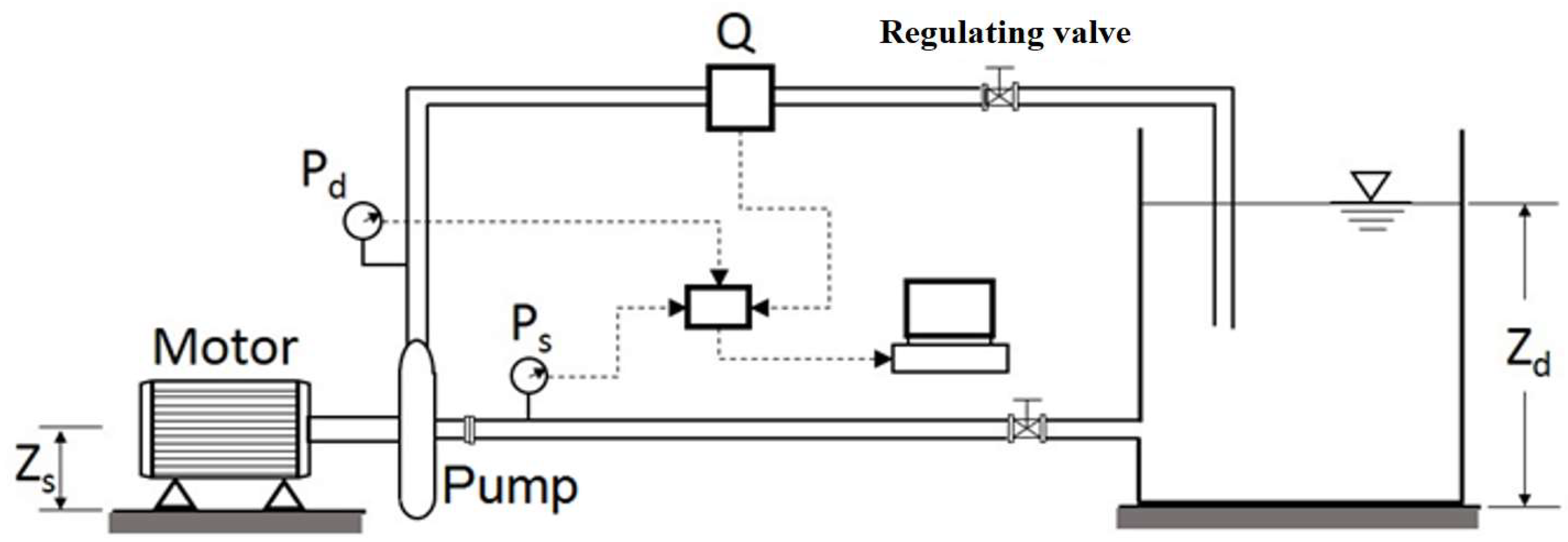
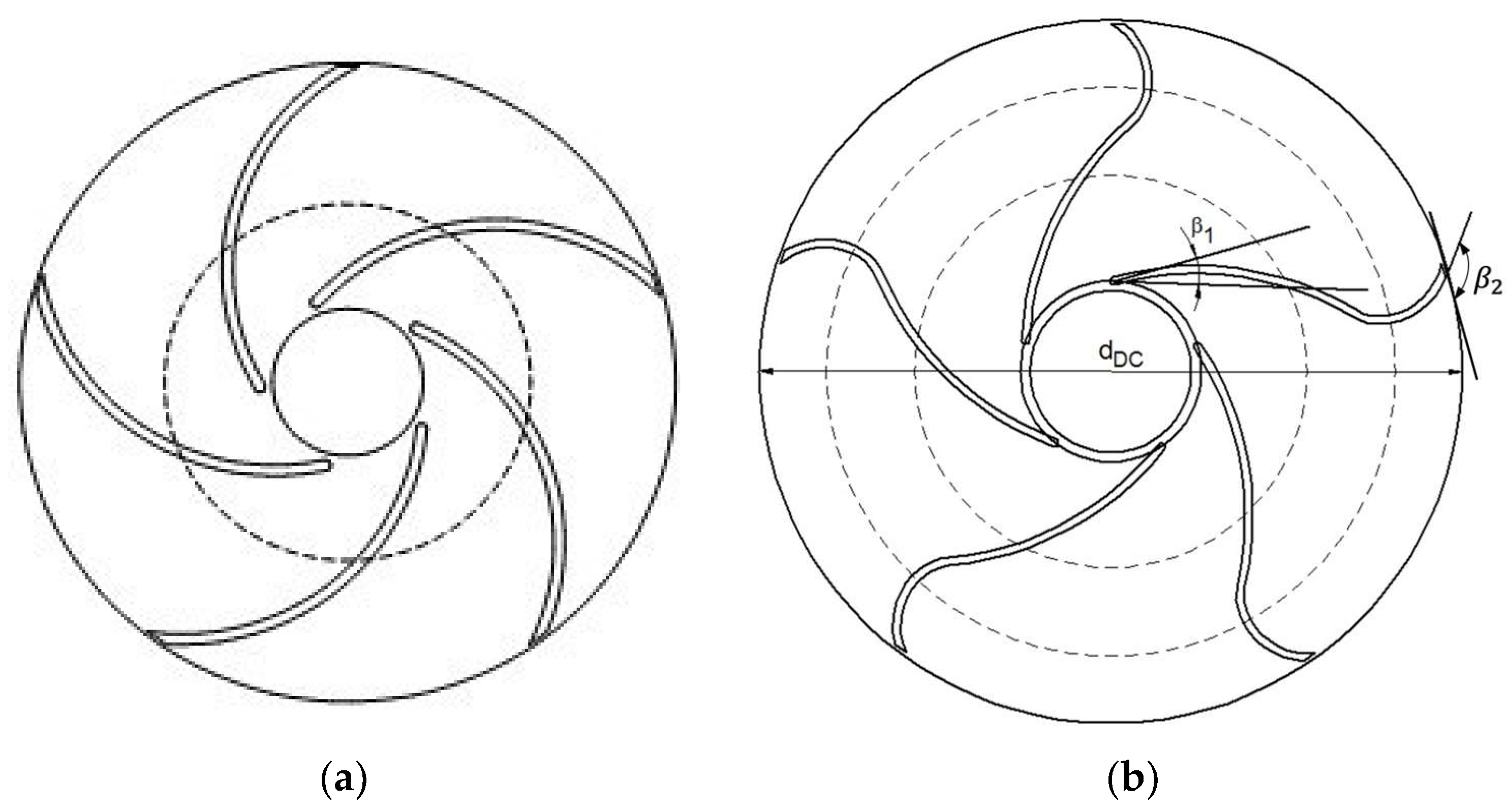
2.1. Experimental Facility, Used Impellers, and Measurements

An experimental facility was configured at the Universidad Tecnológica de Bolívar for testing different impellers. Figure 1 shows the used experimental facility. An IG-IHM Eurolinea 3 × 18 model centrifugal pump with a 2 HP electric motor and 1750 RPM rotational velocity was used in this study. The pump operates at 220 V at 60 Hz.

The experimental facility was built considering ASME PTC 8.2-1990 regulations [49]. The suction ($P_s$) and discharge ($P_d$) pressure and flow ($Q$) were measured online through a program developed in LabView. The program collects 100 data points per second and delivers their average. The motor’s rotational velocity, voltage, current, electrical power, and power factor were also measured.

Autonics high-precision pressure gauges, Signet 8550 flow transmitters, FLUKE 1735 power logger energy analyzer, MDT2238A Minipa digital tachometers, and a variable speed drive were used. Additionally, the experimental facility included two 5000 L tanks with positive suction.

Because forward-curved impellers deliver more head compared to backward-curved impellers but also consume more power, double curvature impellers were designed to produce more head and to study their performance. Experiments were conducted on the original impeller (BO) and with impellers designed, manufactured, and assessed by the authors.

Table 1. Characteristics of the assessed impellers.

Impeller	${\mathit{\beta }}_1$ (°)	${\mathit{\beta }}_2$ (°)	$\mathit{D}\mathit{C}$ (%)	${\mathit{d}}_{\mathit{D}\mathit{C}}$ (mm)
BO	17	30
BOAl	17	30
B25A	90	150	25	159.9
B25B	163	30	25	159.9
B50A	90	150	50	113.2
B50B	163	30	50	113.2
B15B	163	30	15	159.9

shows the characteristics of these impellers, where ${\beta }_1$ is the impeller inlet angle, $DC$ is the double curvature percentage (15%, 25%, or 50%), and $d_{DC}$ is the double curvature’s diameter.

The pump’s original impeller was made of bronze. To compare potential changes that could arise from differences in material and manufacturing processes, an impeller with the same dimensions as the original was built. It was made from aluminum (BOAI). Additionally, five impellers were designed with double curvatures of 15%, 25%, or 50%. The percentage of double curvature was calculated based on the blade’s exterior and interior diameters and measured from the exterior diameter. The impeller’s outlet diameter ($d_2$) is 180 mm, and the inlet diameter ($d_1$) is 46.3 mm. To determine the double curvature’s diameter, the following equation was defined and used by the authors:

$$d_{DC}=d_2-\left(d_2-d_1\right)DC$$

(1)

The configurations of the impellers are presented in Figure 2. The blade shape of the original bronze impeller (BO) and aluminum original impeller (BOAI) are presented in Figure 2a, while Figure 2b illustrates the blade shape of the double curvature impellers. All analyzed impellers had five blades.

The experimental plan consisted of assessing impellers with different configurations and using a variable speed drive, modifying rotational velocities between 1400, 1700, and 1900 RPM, which correspond to operating values normally used in the operation of pump systems.

Before the tests, the pump’s maximal flow rate, $Q_{max}$, (with the regulating valve completely open) for each impeller and each rotational speed was determined. This flow was divided by 11 to determine flow variations ($∆Q$) in Equation (2), which was defined by the authors to divide the maximum flow rate in different testing points.

$$\mathsf{\Delta }Q=\frac{Q_{max}}{n-1}$$

(2)

The flow meter measured the water flow when the regulating valve was opened, ensuring controlled flow for each test to guarantee 12 different flow rates per test that corresponded to 12 points on the chart showing head as a function of flow.

Measurements were taken for the discharge pressure, suction pressure, flow, current intensity per phase, line voltage, power factor, the motor’s electrical power consumption, and angular velocity (RPM) for each position of the regulating valve. To ensure accuracy, a 5 min stabilization period controlled by the program was applied for each valve aperture, followed by a 2 min data collection period.

The input data were the mass flow, outlet’s maximum pressure, and rotational velocity. The rotational velocities used for the experimental tests were used here as well: 1400, 1700, and 1900 RPM. Simulation values correspond to the different points of the experimental tests, i.e., there was a simulation for each flow obtained in the experimental tests for the corresponding valve maneuver.

2.2. Numerical Simulation

2.2.1. Governing Equations

Numerical simulations were performed using STAR-CCM+ (Siemens). A 3D CFD model was used, applying the following assumptions: (i) the flow was composed of a liquid phase (water) being a monophasic and segregated flow with constant density due to the mechanical properties of the water phase as incompressible flow, and (ii) numerical simulation was performed in a steady state. Therefore, transient flows, thermodynamic effects, and heat transfer were neglected in this modelling. The following equations correspond to continuity and momentum equations that represent the movement of fluids [50].

$$\nabla ·\mathbf{V}=0$$

(3)

$$\nabla ·\left(\rho \mathbf{V}\mathbf{V}\right)=-\nabla p+\mu {\nabla }^2\mathbf{V}+\rho \mathbf{g}$$

(4)

where V = velocity vector, ρ = density of liquid, p = static pressure, $\mu$ = dynamic viscosity, and g = gravitational acceleration vector.

The selected turbulence model was k-ε, which is one of the most widely utilized models [51,52]. It is an semi-empirical model based on transport formulations for the turbulent kinetic energy (k) and its corresponding dissipation rate (ε), which can be applied only for fully turbulent flows. Equations (5) and (6) describe the used transport formulations:

$$\frac{\partial }{\partial x_i}\left(\rho k{u}_i\right)=\frac{\partial }{\partial x_j}\left[\left(\mu +\frac{{\mu }_t}{{\sigma }_k}\right)\frac{\partial k}{\partial x_j}\right]+G_k+G_b-\rho ϵ-Y_M+S_k$$

(5)

and

$$\frac{\partial }{\partial x_i}\left(\rho ϵu_i\right)=\frac{\partial }{\partial x_j}\left[\left(\mu +\frac{{\mu }_t}{{\sigma }_{ϵ}}\right)\frac{\partial ϵ}{\partial x_j}\right]+C_{1ϵ}\frac{ϵ}{k}\left(G_k+G_{3ϵ}{G}_b\right)-C_{2ϵ}\rho \frac{{ϵ}^2}{k}+S_{ϵ}$$

(6)

where, $G_k$= the generation of turbulence kinetic energy based on mean velocity gradient; $G_b$ = the generation of turbulence kinetic energy based on buoyancy force; $Y_M$= the contribution of the fluctuating dilatation in compressible turbulence; $C_{1ϵ}$, $C_{2ϵ}$, and $G_{3ϵ}$ are constants used by the turbulence model; ${\sigma }_k$ and ${\sigma }_{ϵ}$ are the turbulence Prandtl numbers for k and ε, respectively; $S_k$ and $S_{ϵ}$ are user-defined source terms; $\rho$ = mixture density; and $\mu$ = mixture dynamic viscosity. The turbulent viscosity (${\mu }_t$) is compued as follows [51]:

$${\mu }_t=\rho C_u\frac{k^2}{ϵ}$$

(7)

where $C_u$ = constant.

On the other hand, the SST k-ω model was used as a complement to compare the influence of generation–dissipation of the turbulence, considering that this model combines the advantages of k-ε and standard k-ω models. Equations (8) and (9) correspond to generation and dissipation of turbulence, respectively [53,54].

$$\frac{\partial }{\partial x_i}\left(\rho k{u}_i\right)=\frac{\partial }{\partial x_j}\left[\left(\mu +{{\mu }_t\sigma }_k\right)\frac{\partial k}{\partial x_j}\right]+P_k-\beta *\rho k\omega$$

(8)

$$\frac{\partial }{\partial x_i}\left(\rho \omega u_i\right)=\frac{\partial }{\partial x_j}\left[\left(\mu +{{\mu }_t\sigma }_{\omega }\right)\frac{\partial k}{\partial x_j}\right]+\alpha \frac{1}{{\nu }_t}{P}_k-\beta \rho {\omega }^2+2\left(1-F_1\right)\rho {\sigma }_{\omega 2}\frac{1}{\omega }\frac{\partial k}{\partial x_j}\frac{\partial \omega }{\partial x_j}$$

(9)

where ω = dissipation frequency, P_k = generation of turbulence, F₁ = blending function, ν_t = turbulent kinetic viscosity, and terms such as α, β, β* σ_k and σ_ω are constants that correspond to the turbulence model.

The SST k-ω model has been used in the literature to simulate impellent in pump systems [55,56], as well as the k-ε model [55,57]. Therefore, it is appropriate to perform a comparison of the generation and dissipation of turbulent effects in centrifugal pump impellers.

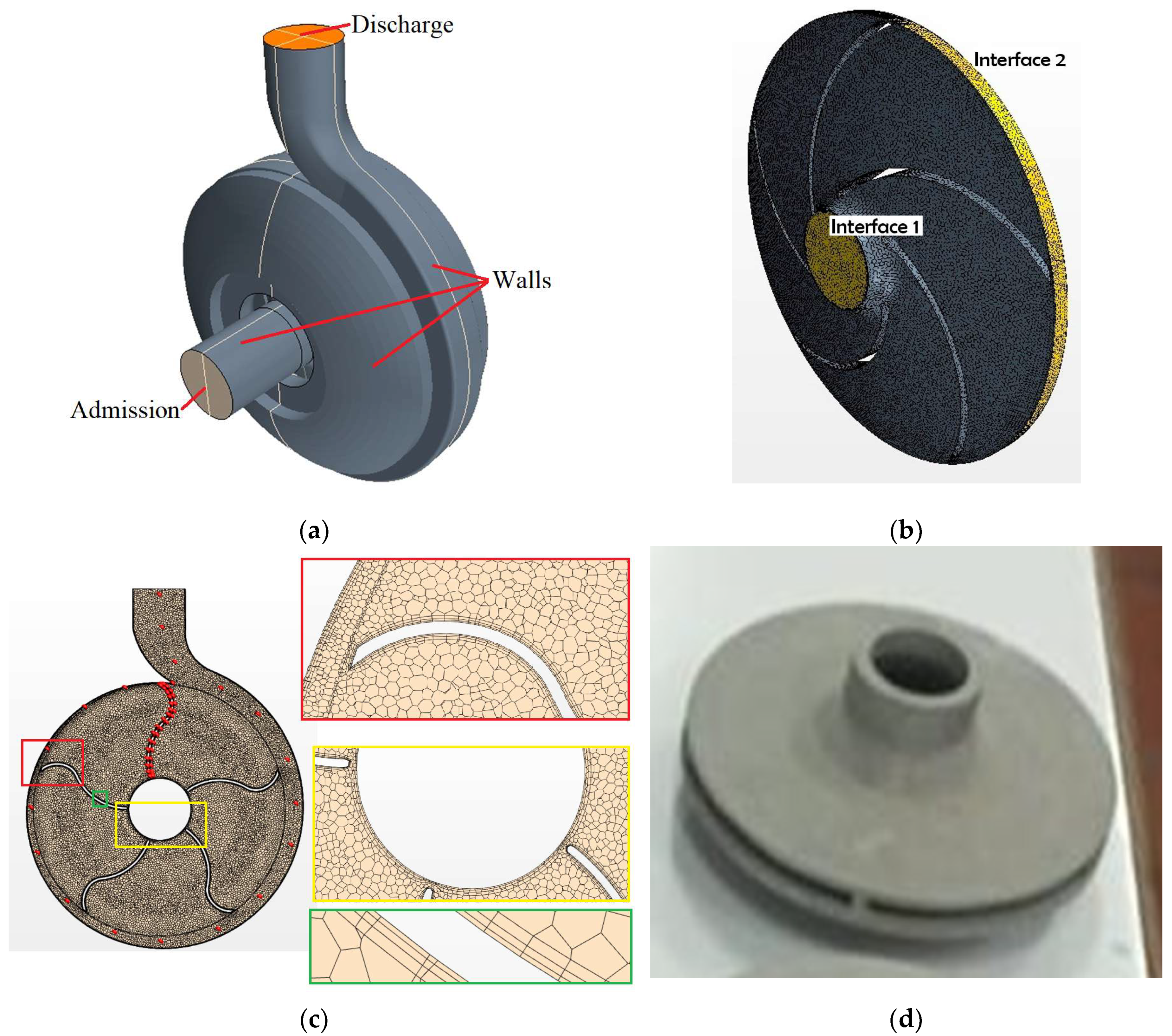
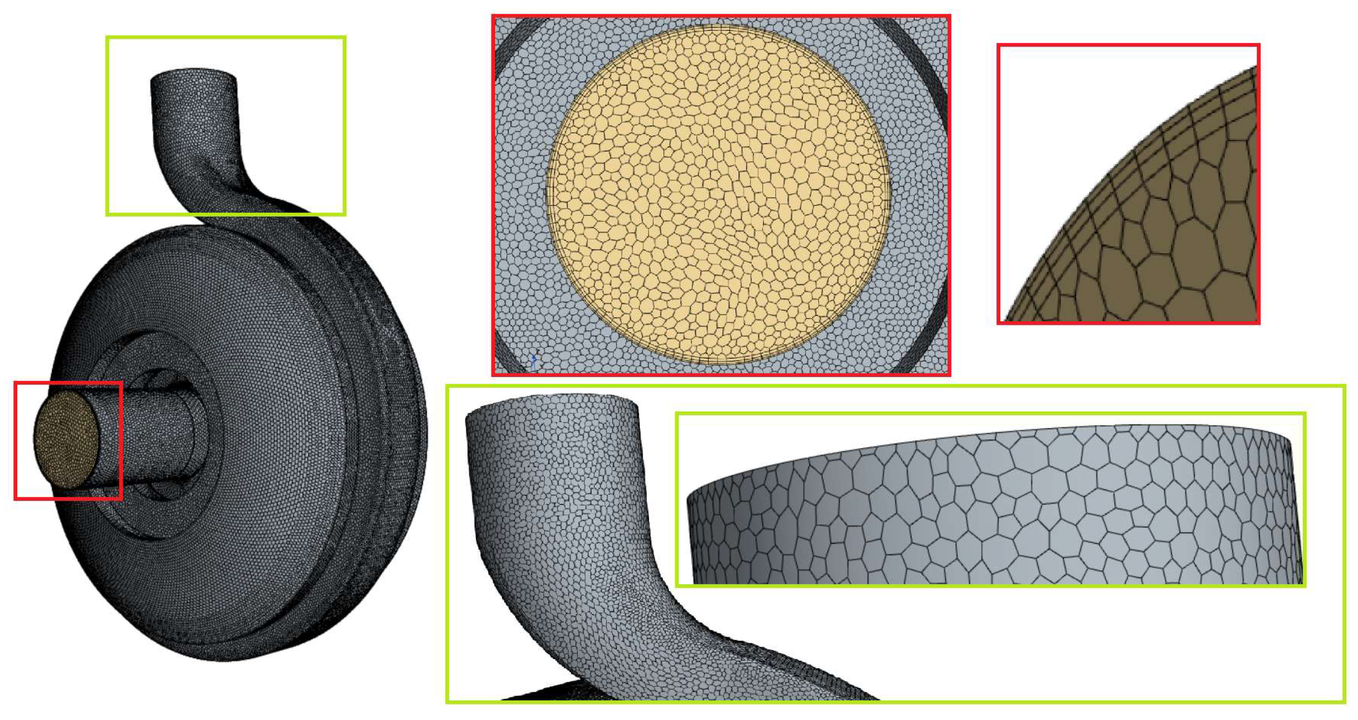
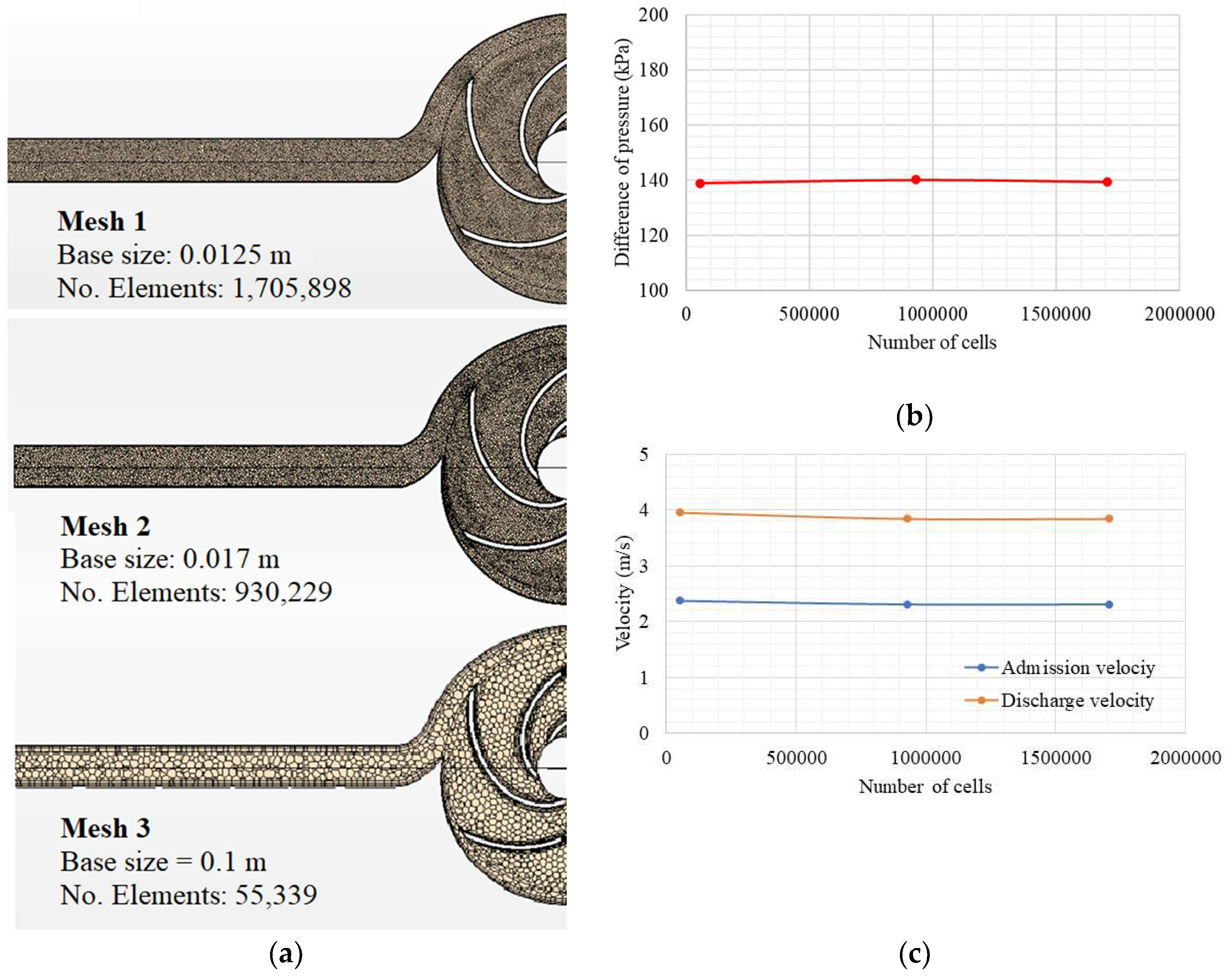
2.2.2. Geometric, Mesh, and Boundary Conditions

The assessed impellers, volute, and part of the suction and discharge branch pipes were digitized using Solid Edge ST5. The imported solid represents the system’s fluid composed by different boundaries: (i) admission, where flow is admitted to geometric domain applying a mass flow rate; (ii) discharge, which is the boundary where the flow leaves the geometric domain, and the initial condition of velocity and pressure were 0 m/s and 101.325 Pa (1 atm) respectively; and (iii) walls, which guarantees the confinement of the flow within the geometrical domain (see Figure 3a). Two interfaces were created to allow for the exchange of properties between these two areas, as shown in Figure 3b. Interface 1 facilitates the exchange of properties in the fluid as it enters the impeller from the volute inlet, while interface 2 enables the exchange of properties in the fluid exiting the impeller and entering the volute.

In this simulation, an unstructured mesh was applied, where polyhedral cells were used in Rotating Fluid region and Fluid Region as shown in Figure 3c and Figure 4, respectively, where structured cells were detailed at the near-wall boundary layer with a wall distance of 0.2 mm and an aspect ratio of 0.65. In addition, Figure 3d shows an example of a real impeller, which was used in the laboratory.

To define the size of mesh, a mesh independence analysis was performed using three (3) different meshes to verify the independence of numerical results of mesh conditions, where Impeller BO was tested, in this case. To generate the meshes, a value of base size was assigned for different meshes, as shown in Figure 5a. For the entire study, the stopping criteria used for residuals was 1 × 10⁻⁴. Parameters such as difference in pressure and velocity of admission and discharge were evaluated for different scenarios. Figure 5b shows the variation of difference in pressure, where it was observed that these values ranged between 139 and 140.3 kPa considering the meshes used that considered cell numbers between 55,339 and 1,705,898, with insignificant changes in the pressure difference as a function of the number of cells, being an acceptable trend from a numerical point of view. On the other hand, Figure 5c shows that admission and discharge velocity presented a few variations in their values considering the number of cells used in the CFD model, being that the values of admission velocity were between 2.30 and 2.37 m/s, and the values of discharge velocity were between 3.85 and 3.95 m/s. Therefore, the velocity results also behaved adequately regardless of the mesh resolution.

Finally, it was possible to identify the independence of numerical results from the resolution of the mesh, so that the choice of the number of cells in this case was determined according to the resolution of the information to be visualized. In that sense, the size of the volumetric polyhedral meshes obtained after the mesh independence analysis was 0.015 m (Between Mesh 1 and 2), which was obtained for each section of the different cells and node quantities of the assessed impellers (see

Table 2. Number of cells and nodes for each area.

Impeller	Fluid		Rotating Fluid
	Cells	Nodes	Cells	Nodes
BO/BOAl	776,181	4,243,191	217,590	1,088,747
B25A	776,005	4,238,226	216,562	1,099,660
B25B	774,347	4,227,560	224,197	1,122,148
B50A	779,221	4,260,653	213,663	1,083,460
B50B	777,577	4,250,597	223,323	1,122,050
B15B	771,334	4,208,591	227,538	1,138,883

).

Simulations were performed using an HP computer with 32 cores and 256 GB of RAM. The simulation time was around 12 h.

3. Analysis of Results

Considering that two impellers have a similar geometry (the original impeller in bronze and the aluminum one), seven impellers were experimentally assessed, and six impellers were simulated using a 3D CFD model. Tests were conducted at three different speeds (1400 RPM, 1700 RPM, and 1900 RPM).

3.1. Experimental Curves

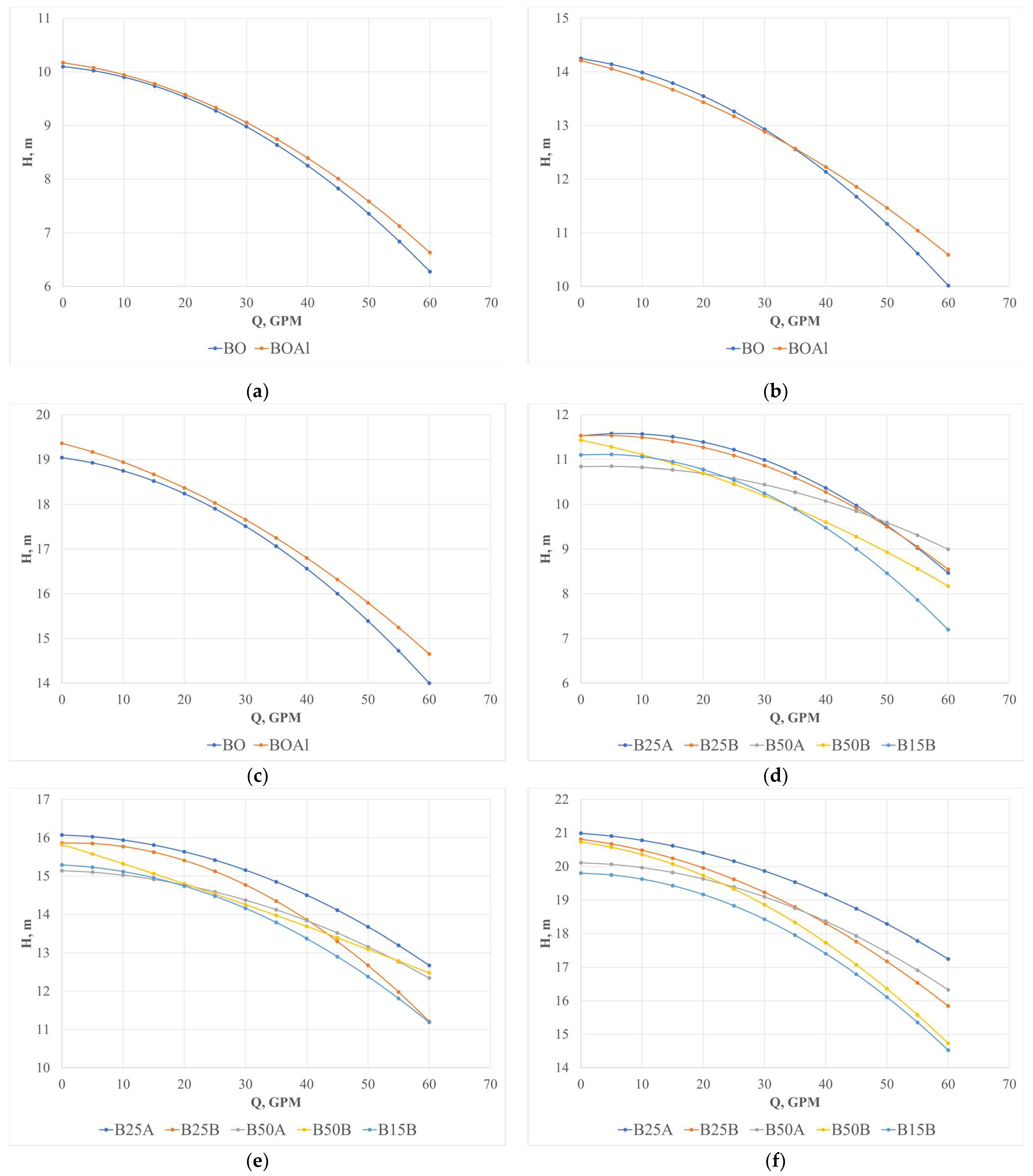
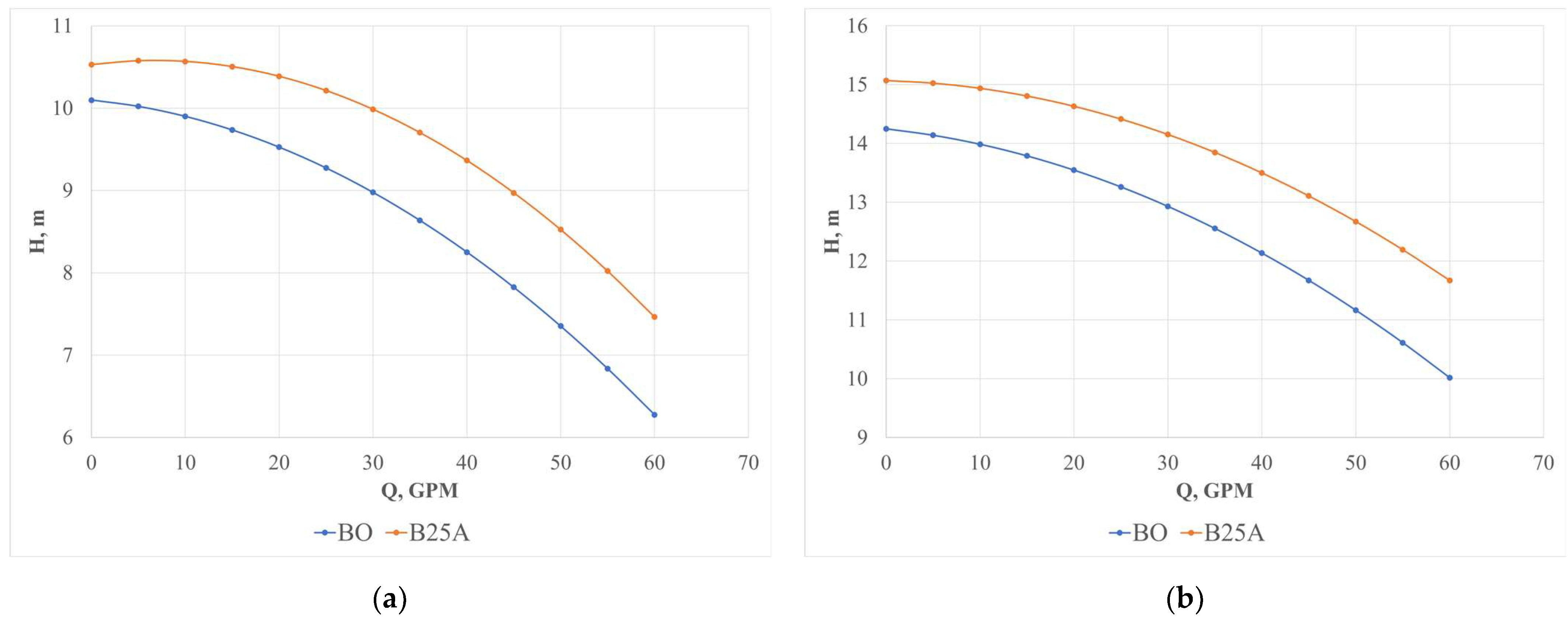
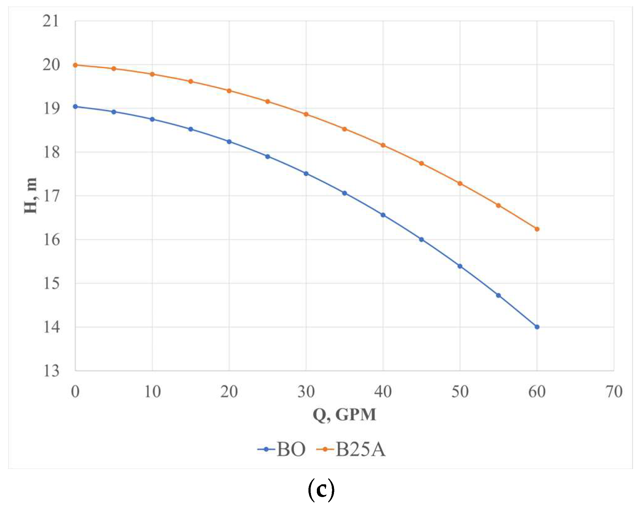
3.1.1. Head–Flow Rate Curve

The following data were measured at 12 points per impeller and for each rotational velocity: suction pressure, discharge pressure, rotational velocity, flow rate, voltage, electric current, power factor, and electrical power. Based on these data, the Bernoulli equation was applied to compute the pump head [58]:

$$H=\frac{P_d-P_s}{{\gamma }_w}+\frac{V_d^2-V_s^2}{2g}+(Z_d-Z_s)$$

(10)

where $H$ is the pump head; $P_d$ and $P_s$ are the discharge and suction pressures, respectively; $V_d$ and $V_s$ are the discharge and suction velocities, respectively; $Z_d$ and $Z_s$ are the discharge and suction heights, respectively; and ${\gamma }_w$ is the water specific weight. Figure 4 shows the measurement points for each variable. Once the head for each point was calculated, the head–flow rate equation was determined. The analyzed head–flow rate equation is shown below [58]:

$$H=A{Q}^2+BQ+C$$

(11)

Constants $A$, $B$, and $C$ for the assessed impellers are shown in

Table 3. Constants for the pump head–flow rate of the assessed impellers.

Impeller	w (RPM)	$\mathit{A}$	$\mathit{B}$	$\mathit{C}$	R2
BO	1400	−8.77 × 10−4	−1.11 × 10−2	10.10	98.98
	1700	−8.86 × 10−4	−1.74 × 10−2	14.25	99.76
	1900	−1.10 × 10−3	−1.80 × 10−2	19.04	99.80
BOAl	1400	−7.28 × 10−4	−1.53 × 10−2	10.17	99.90
	1700	−5.37 × 10−4	−2.81 × 10−2	14.21	99.93
	1900	−7.23 × 10−4	−3.51 × 10−2	19.36	99.94
B25A	1400	−1.10 × 10−3	1.49 × 10−2	10.53	98.83
	1700	−8.69 × 10−4	−4.50 × 10−3	15.07	99.67
	1900	−8.29 × 10−4	−1.27 × 10−2	19.99	99.46
B25B	1400	−9.16 × 10−4	5.20 × 10−3	10.53	98.36
	1700	−1.37 × 10−3	4.75 × 10−3	14.86	98.37
	1900	−1.00 × 10−3	−2.28 × 10−2	19.81	99.80
B50A	1400	−5.81 × 10−4	4.09 × 10−3	9.84	97.61
	1700	−7.00 × 10−4	−4.62 × 10−3	14.14	99.34
	1900	−9.72 × 10−4	−4.78 × 10−3	19.11	95.24
B50B	1400	−4.32 × 10−4	−2.84 × 10−2	10.43	97.28
	1700	−1.15 × 10−4	−4.88 × 10−2	14.82	96.59
	1900	−1.25 × 10−3	−2.50 × 10−2	19.73	99.55
B15B	1400	−1.22 × 10−3	8.15 × 10−3	10.10	98.06
	1700	−1.02 × 10−3	−7.20 × 10−3	14.29	98.91
	1900	−1.40 × 10−3	−3.91 × 10−3	18.80	99.47

. In addition, the correlation coefficient (R²) was calculated for each test. A minimum value of 95.24% was found for the impeller B50A with 1900 RPM, while a maximum value of 99.94% was computed for the impeller BOAl (1900 RPM). These values showed that the model is suitable to represent these experimental curves. Figure 6a–c show the head–flow rate curves for the original impeller and the aluminum impeller with the same geometry for each velocity tested. Figure 6d–f show the head–flow rate curve for impellers B25A, B25B, B50A, B50B, and B15B for each velocity tested.

Table 4. Impeller maximum flow rate (GPM) for each rotational velocity.

Impeller	w (RPM)
	1400	1700	1900
BO	37.95	45.33	51.82
BOAl	37.96	45.42	52.08
B25A	39.41	46.98	53.60
B25B	39.35	43.47	52.07
B50A	38.97	46.22	52.84
B50B	37.06	45.08	50.80
B15B	37.31	44.56	50.55

shows the impellers’ maximum flow rates (GPM) for each rotational velocity.

Table 4 shows the maximum flow rates obtained using different impellers.

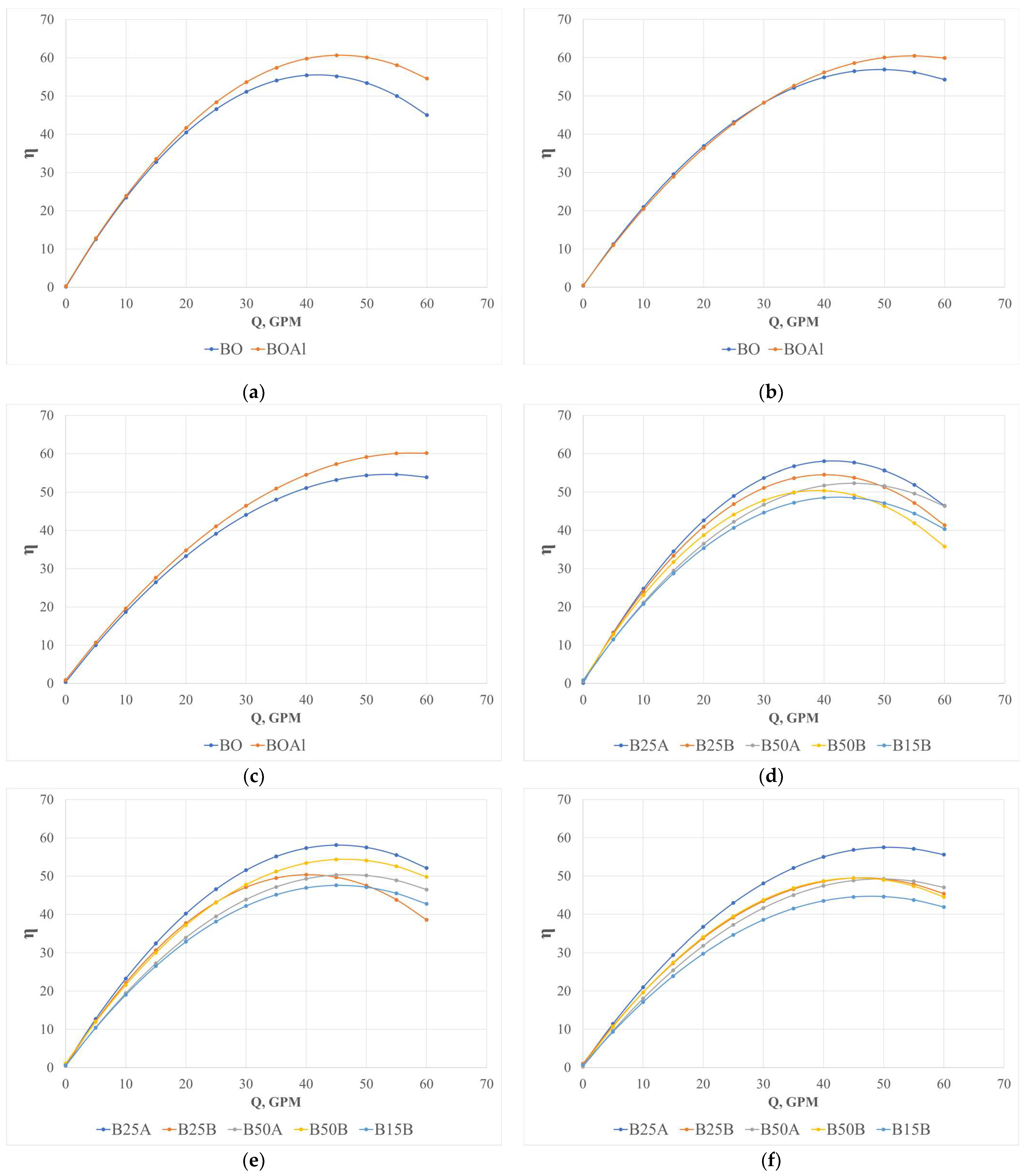
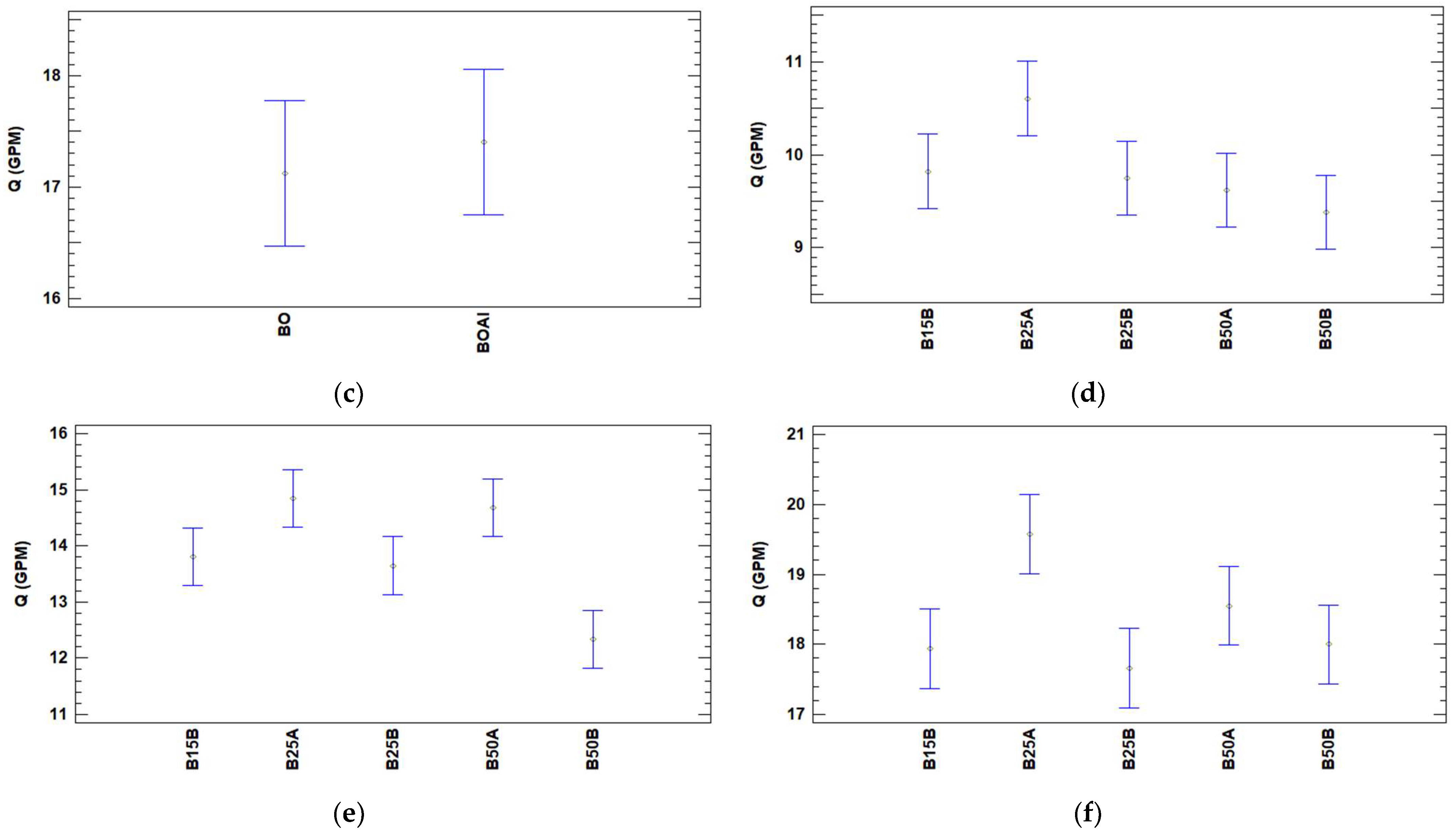
3.1.2. Performance–Flow Rate Curve

The pump–motor unit’s performance was calculated using the following equation [58]:

$$\eta =\frac{QH{\gamma }_w}{N_e}$$

(12)

where $\eta$ is the pump–motor unit performance, and $N_e$ is the measured electrical power.

Once the performance for each point was calculated, the performance as a function of flow rate was determined. Figure 7a–c show the performance as a function of flow rate for the original impeller and the aluminum original impeller for each velocity tested. Figure 7d–f show the performance as a function of flow rate for impellers B25A, B25B, B50A, B50B, and B15B for each velocity tested.

The performance–flow rate equation was:

$$\eta =D+EQ+F{Q}^2$$

(13)

The values of the constants for the assessed impellers are listed in

Table 5. Performance constants for the pump–motor unit as a function of flow rate of the assessed impellers.

Impeller	w (RPM)	D	E	F	R2
BO	1400	−3.17 × 10−2	2.65	1.27 × 10−1	99.99
	1700	−2.32 × 10−2	2.29	4.01 × 10−1	99.97
	1900	−1.88 × 10−2	2.02	3.71 × 10−1	99.98
BOAl	1400	−2.91 × 10−2	2.65	3.10 × 10−1	99.95
	1700	−2.00 × 10−2	2.19	5.46 × 10−1	99.95
	1900	−1.77 × 10−2	2.05	8.68 × 10−1	99.90
B25A	1400	−3.38 × 10−2	2.80	1.22 × 10−1	99.71
	1700	−2.79 × 10−2	2.53	7.61 × 10−1	99.90
	1900	−2.21 × 10−2	2.24	7.74 × 10−1	99.92
B25B	1400	−3.35 × 10−2	2.69	5.53 × 10−1	99.91
	1700	−3.06 × 10−2	2.47	5.17 × 10−1	99.86
	1900	−2.25 × 10−2	2.09	9.85 × 10−1	99.73
B50A	1400	−2.58 × 10−2	2.31	6.18 × 10−1	99.93
	1700	−2.27 × 10−2	2.13	3.94 × 10−1	99.92
	1900	−2.00 × 10−2	1.98	2.23 × 10−1	99.13
B50B	1400	−3.28 × 10−2	2.55	8.57 × 10−1	99.73
	1700	−2.48 × 10−2	2.30	1.08	99.55
	1900	−2.36 × 10−2	2.15	4.88 × 10−1	99.89
B15B	1400	−2.67 × 10−2	2.26	8.55 × 10−1	99.40
	1700	−2.28 × 10−2	2.07	6.11 × 10−1	99.89
	1900	−1.92 × 10−2	1.84	6.24 × 10−1	99.91

; likewise, each equation shows a correlation coefficient with values greater than 99%, which indicates that the computed equation is highly suitable.

4. Discussion

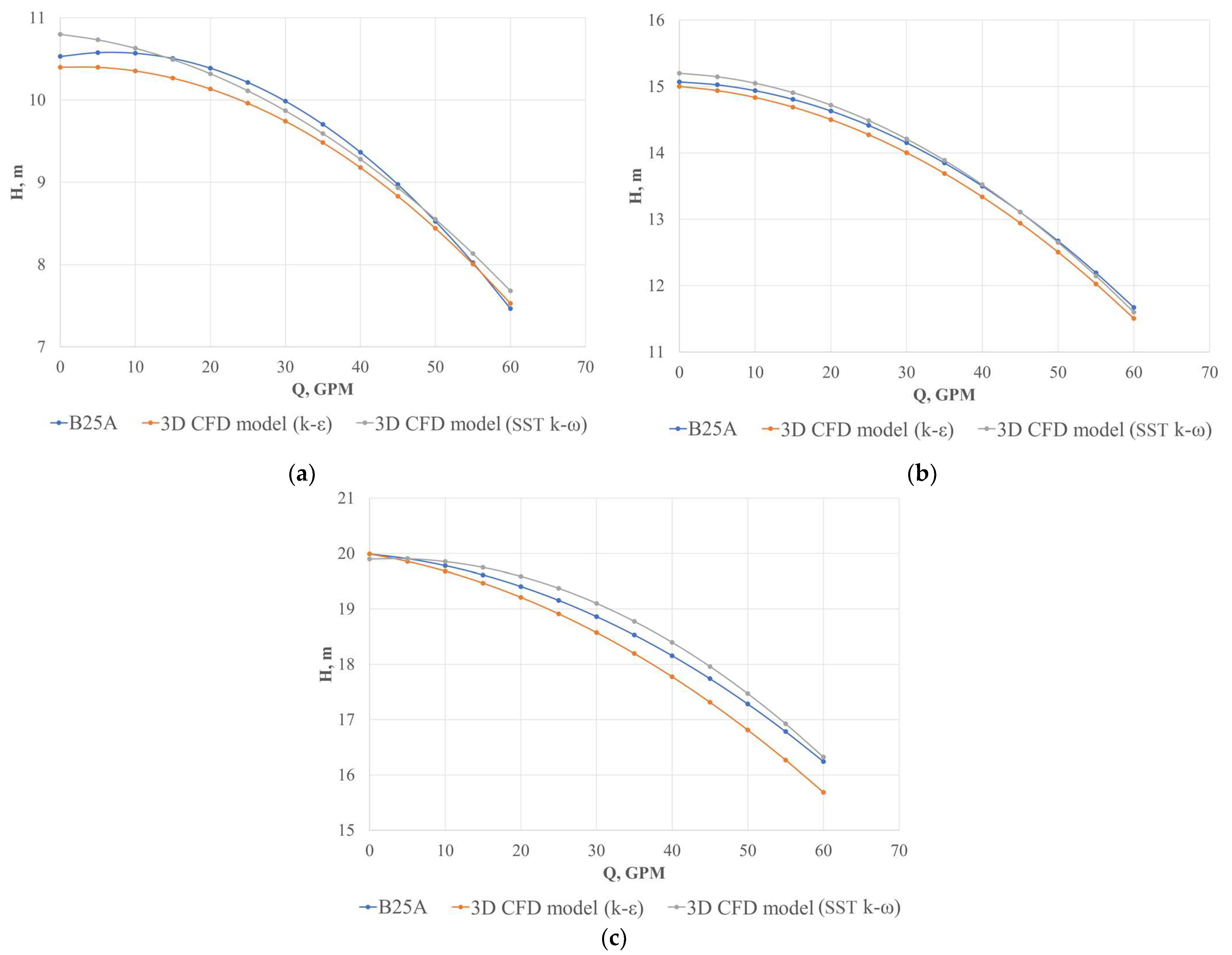
4.1. Head–Flow Rate Curves

The Tukey’s test (HSD) is the test most applied and preferred by statisticians because it better controls the two widely known statistical errors (Type I and Type II) [59]. Figure 6a–c show the head–flow rate curves for impellers BO and BOAl for each velocity tested. The maximum flow rate difference obtained between both impellers was 0.26 GPM at 1900 RPM. No significant differences between impellers BO and BOAl were found. Based on Tukey’s test, it can be concluded that double curved impellers can be made from aluminum because neither the material of the impeller nor the manufacturing process affects the pump’s head when compared to that of the bronze impeller. Figure 8d–f show better performance in relation to head delivered by impeller B25A.

A comparison of head–flow rate curves between impellers BO and B25A was conducted. Figure 9a–c show the results for each velocity applied in the experiment measurements. Impeller B25A performed better than the original impeller in terms of head. Figure 10a–c show that impeller B25A performed better than the original impeller (BO) in terms of head, with a 95% confidence level per Tukey’s test. However, this difference decreased as the rotational velocity increased. Based on the results, a flow rate of 30 GPM (at 1500 RPM) gives a height difference of 1.0 m between BO and B25A impellers; with 1700 RPM, a height difference of 1.23 m is obtained; and for 1900 RPM, a height difference of 1.36 m is attained. Similarly, considering a flow rate of 50 GPM for speeds of 1500 RPM, 1700 RPM, and 1900 RPM, height differences of 1.17, 1.53, and 1.90 are computed, respectively.

4.2. Performance–Flow Rate Curve

A comparison between performance–flow rate curves has been analyzed to detect the best impeller. Figure 11 shows a slightly improved performance for the original aluminum impeller (BOAl) compared with that of the original bronze impeller (BO) at all tested velocities. The original bronze impeller (BO) and the original aluminum impeller (BOAl) have a similar performance according to Tukey’s test. Figure 11 shows better performance by impeller B25A. Tukey’s test for double curvature impellers (B25A, B25B, B50A, B50B, and B15B) shows no statistically significant difference among them. Although there is no significant statistical difference between the considered impellers, it is important to highlight that the impeller B25A yields an average performance of 42% for the different tested speeds, while the OB impeller reached a value of 40%.

Figure 12a–c show the performance of the pump–motor unit for impellers BOAl and B25A. A slightly better performance is observed for impeller BOAl compared with impeller B25A for each tested velocity.

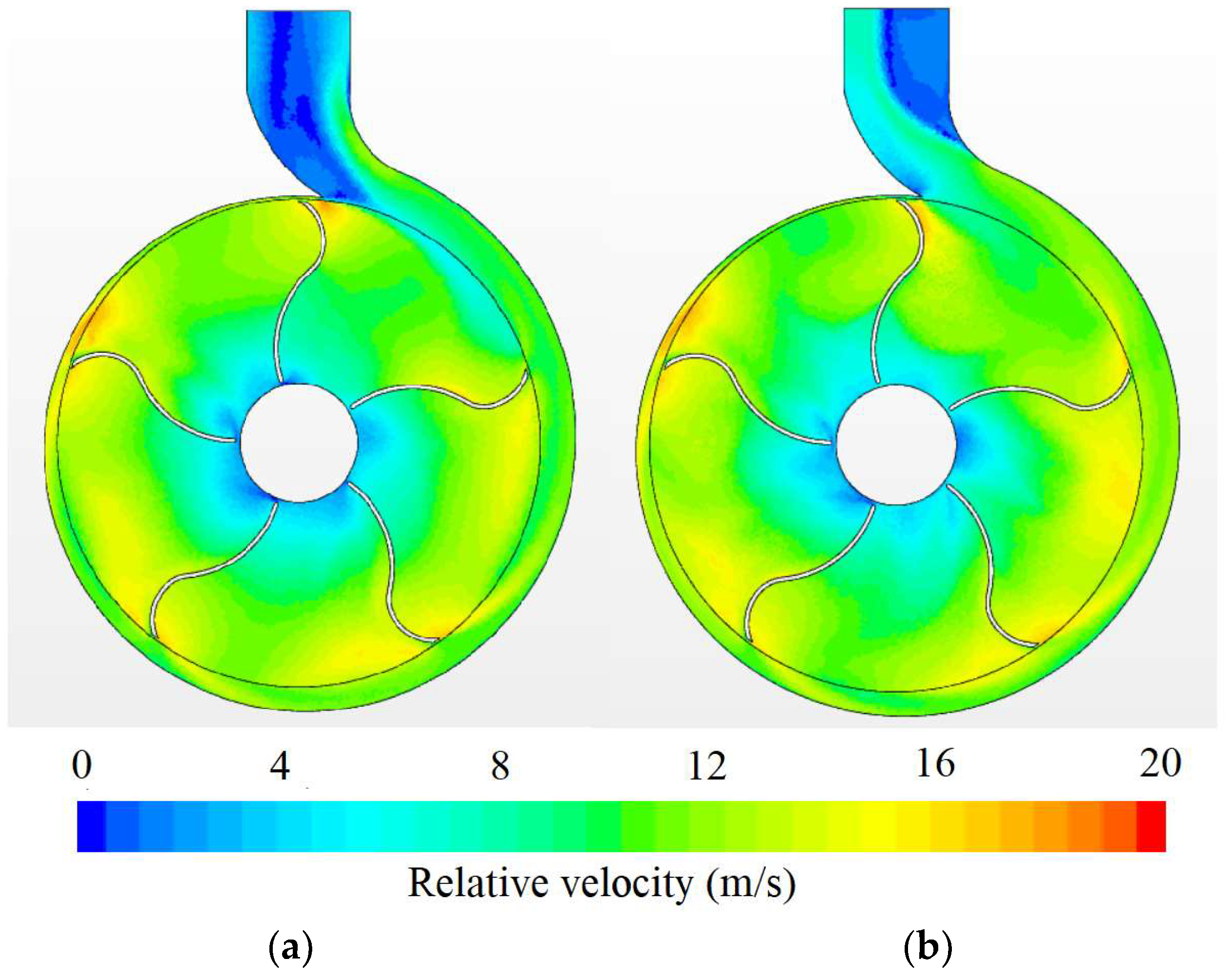
4.3. Phenomenon Description and CFD Validation

The numerical simulation shows the pump’s interior flow and allows for an analysis of its interior phenomena. Figure 13 shows the pump’s pressure distribution when using impellers B25A and BO, and, as expected from a centrifugal pump, the pressure of both impellers increases from the center of the impeller to the blade outlet; however, for similar flow rates, higher pressure at the pump’s outlet is observed when using impeller B25A. At the outlet of the volute, pressures around 200 kPa can be reached for the casing of impeller B25A, while, for the original impeller (BO), the pressures are around 150 kPa. Figure 14 shows an increase in pressure as the fluid travels from the inlet to the outlet of the volute.

Figure 15 shows the pump’s relative velocity vectors when using impellers B25A and BO at 1700 RPM. Impeller BO shows areas of turbulence, which are larger compared to impeller B25A. Thus, impeller B25A provides a better head and performance behavior regarding flow rate compared to the other ones. In addition, water velocities around 10 m/s can be observed at the outlet of the volute for both impellers, before coming into the diffuser.

A comparison between 3D CFD and experimental results was performed as shown in Figure 16. The impellers B15B, B25A, and BO were selected for conducting the analysis. For all cases, the 3D CFD model is suitable for representing the head curves, since blue lines (experimental test) are similar compared to red lines (3D CFD model).

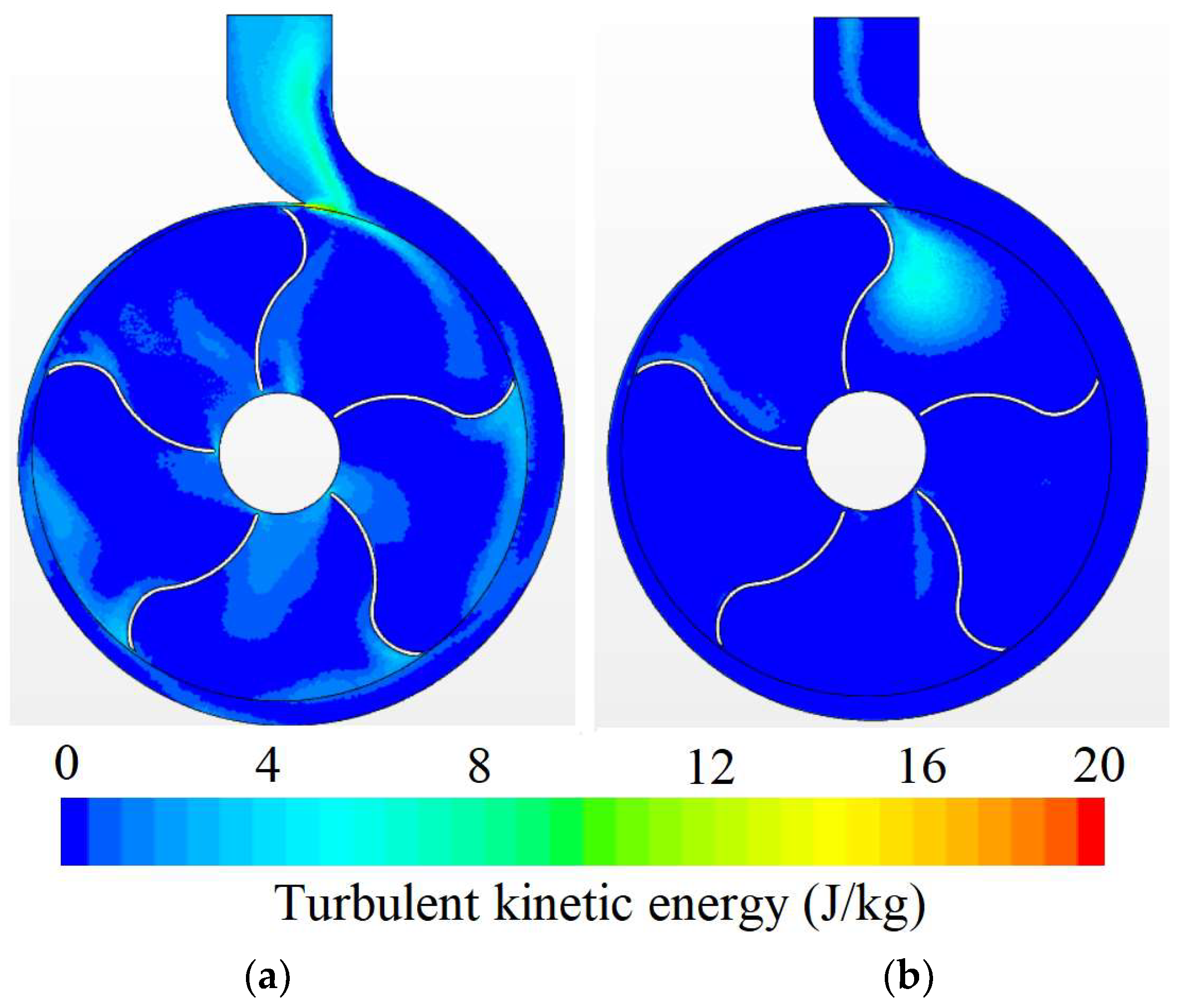
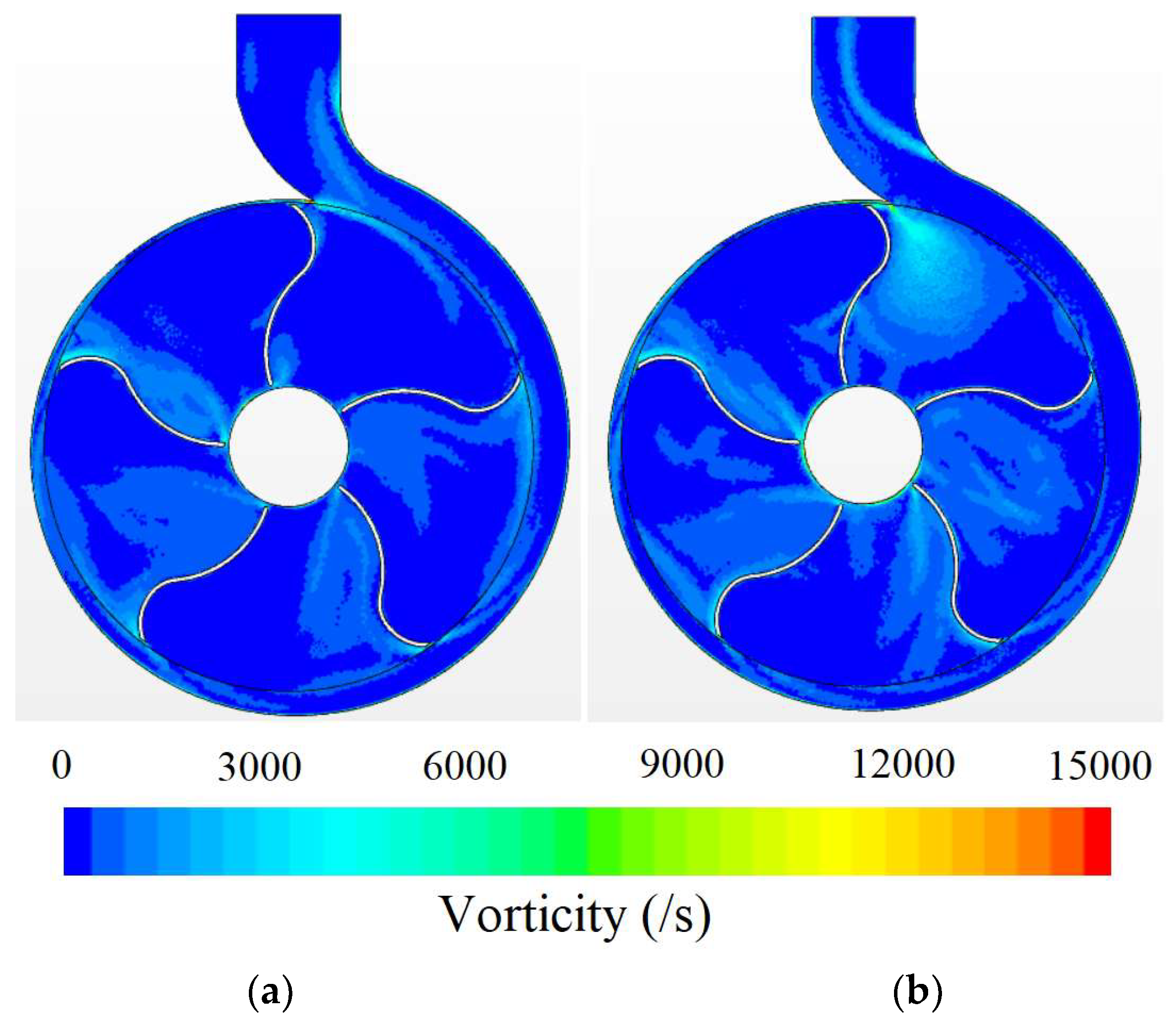
4.4. Comparison between k-ε and SST k-ω Turbulence Models

In this research, a comparison was performed of the pumping curves obtained with the B25A impeller using the k-ε, turbulence model, and the SST k-ω turbulence model to understand the differences in physical and numerical results in applying these models. Figure 17 showed a suitable agreement between the pumping curves applied with the B25A impeller for 1400, 1700, and 1900 RPM. The blue lines represent experimental tests.

Figure 17a showed that the curves obtained from the CFD model with the k-ε and SST k-ω turbulence models presented a similar trend to the experimental curve, where the SST k-ω model curve started from H = 10.8 m, compared to the experimental curve (H = 10.56 m), and the k-ε model curve (H = 10.45 m), and it remained above these in the different Q vs. H. This trend of the pump curve with the SST k-ω model higher than the experimental and CFD model curves with the k-ε turbulence model occurred using other angular velocities (1700 RPM and 1900 RPM), whereas there was a discrepancy between the turbulence model curves in the scenario in Figure 17c (B25A at 1900 RPM).

Figure 18 shows the spatial distribution of pressure in the test with the B25A impeller subjected to 1700 RPM using the k-ε (Figure 18a), and SST k-ω (Figure 18b) turbulence models. There was a significant difference in the prediction of low-pressure zones, mostly noticeable in the results presented by the SST k-ω model, and a higher-pressure gradient at the change of direction, which reaches up to 213,000 Pa, while, with the k-ε model, the pressure at the volute outlet does not exceed 203,000 Pa. Although the turbulence prediction differs in areas such as the low-pressure points on the impeller axis and the volute outlet, the Q vs. H ratio tends to be similar in both turbulence models, as observed in Figure 17b.

In addition, Figure 19 shows the differences in the velocity distribution over the impeller and outlet of the centrifugal pump, where a similar behavior was evidenced over the rotor area from the shaft to the interface of the impeller with the volute. However, there was a difference in the velocity distribution in the discharge area, where it was observed with the k-ε turbulence model (Figure 19a). On the other hand, the result presented by the SST k-ω model (Figure 19b) shows a velocity profile that was presented to a greater extent on the wall of the left sector of the discharge pipe, with velocity values of around 8 m/s, showing an adequate trajectory from the physical point of view.

On the other hand, CFD modelling made it possible to visualize the behavior of some variables associated with the turbulence phenomena occurring in the impeller and the outlet of the volute. In that sense, parameters such as turbulent kinetic energy (Figure 20) and vorticity (Figure 21) were analyzed to compare the effects generated according to the turbulence models.

It was evident that the k-ε turbulence model favored a higher turbulent kinetic energy generation compared to the SST k-ω turbulence model (Figure 20a), considering that this model uses the velocity gradients calculated in the whole system analyzed to capture this phenomenon, while the SST k-ω model predicted the generation of kinetic energy from the generation of shear forces on the fluid, as can be seen in the connection of one of the blades and the connection of the volute with the discharge pipes (see Figure 20b).

In contrast to the turbulent kinetic energy, the vorticity magnitude was higher in the CFD model simulated with the SST k-ω turbulence model (Figure 21b), showing that vortices predominated between blades with a frequency between 3000 and 6000 cycles per second (Hz), while, with the k-ε turbulence model (Figure 21a), the vorticity was located specifically at the impeller blades and with a lower magnitude than that presented in the SST k-w turbulence model, where values below 3000 Hz predominated.

5. Conclusions

This study analyzed pump head and performance as a function of flow rate for double curvature impellers and the pump’s original impeller. For this purpose, an aluminum impeller was built with the same design as the original bronze impeller, and five impellers were created with double curvatures.

Based on this analysis, the following conclusions can be drawn:

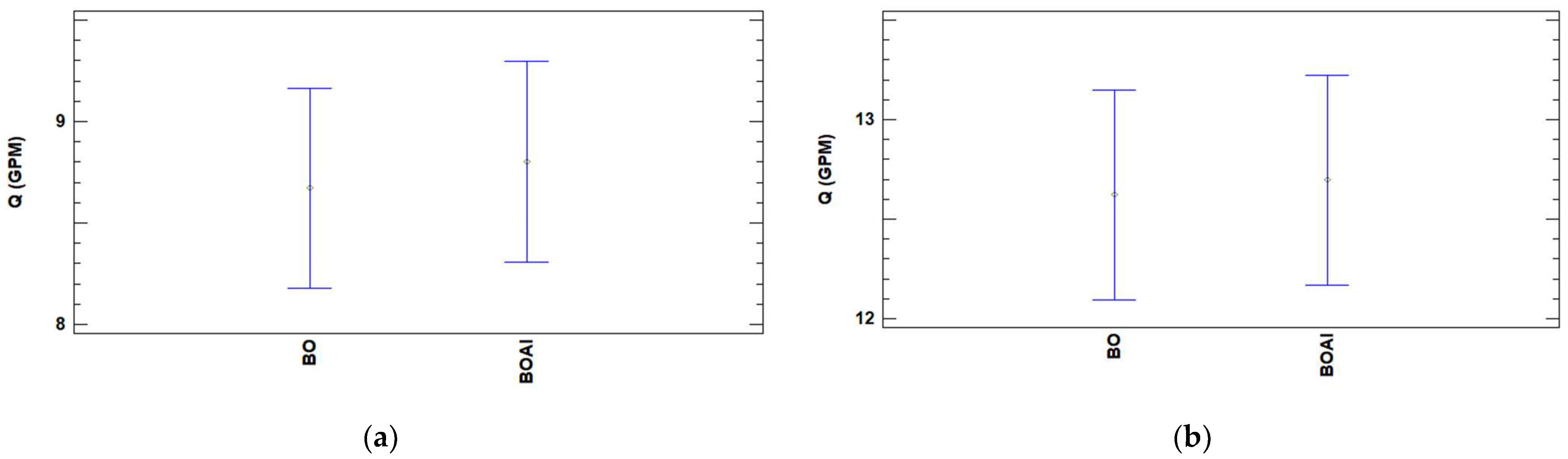
• The head–flow rate and performance–flow rate curves for the original aluminum impeller and original bronze impeller, which came with the pump, are not different; this result validates the comparison of the original bronze impeller with the double curvature impellers. Another important contribution of this study is the set of different head–flow rate and performance–flow rate equations obtained for each of the assessed impellers, both experimentally and by simulation.
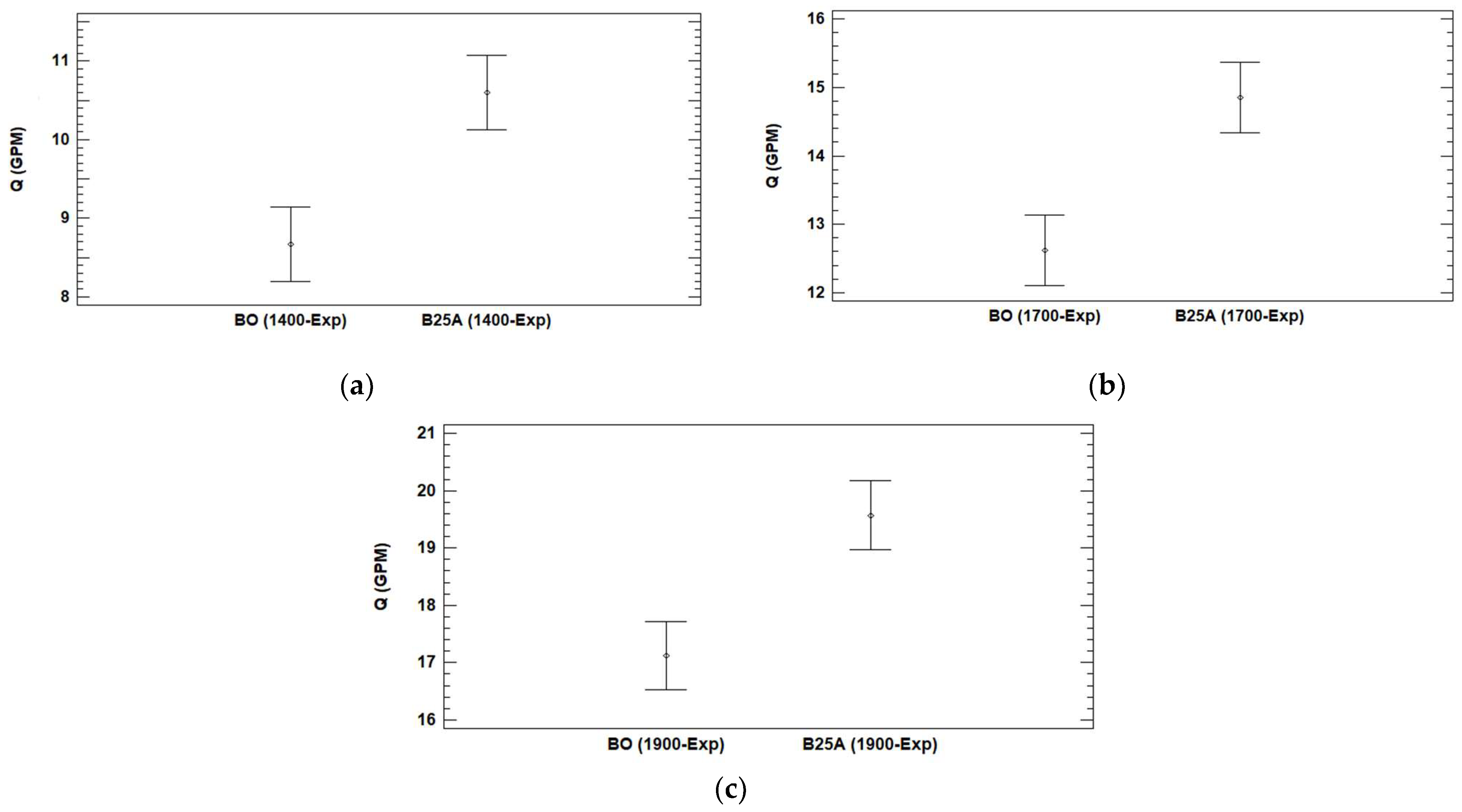
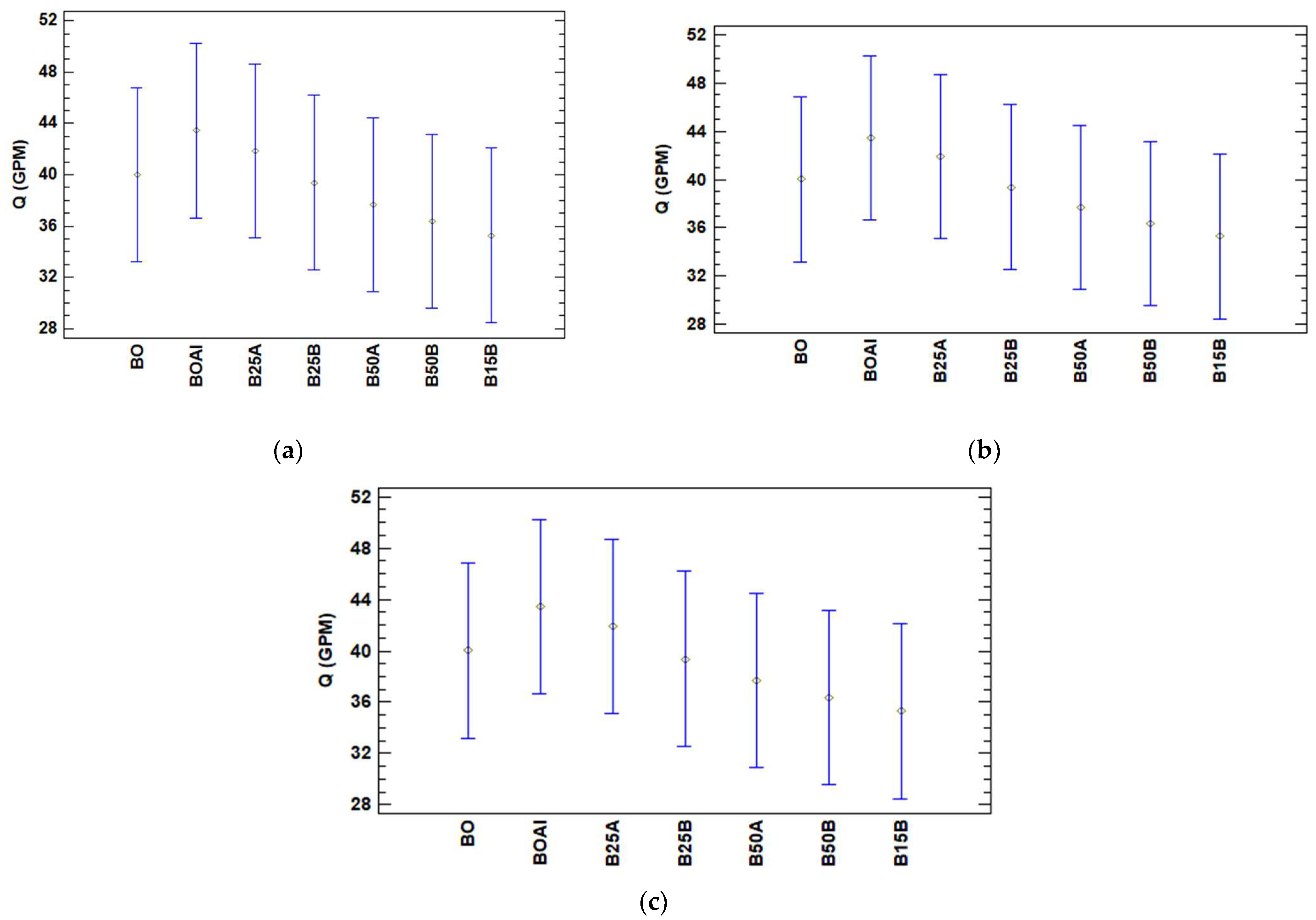
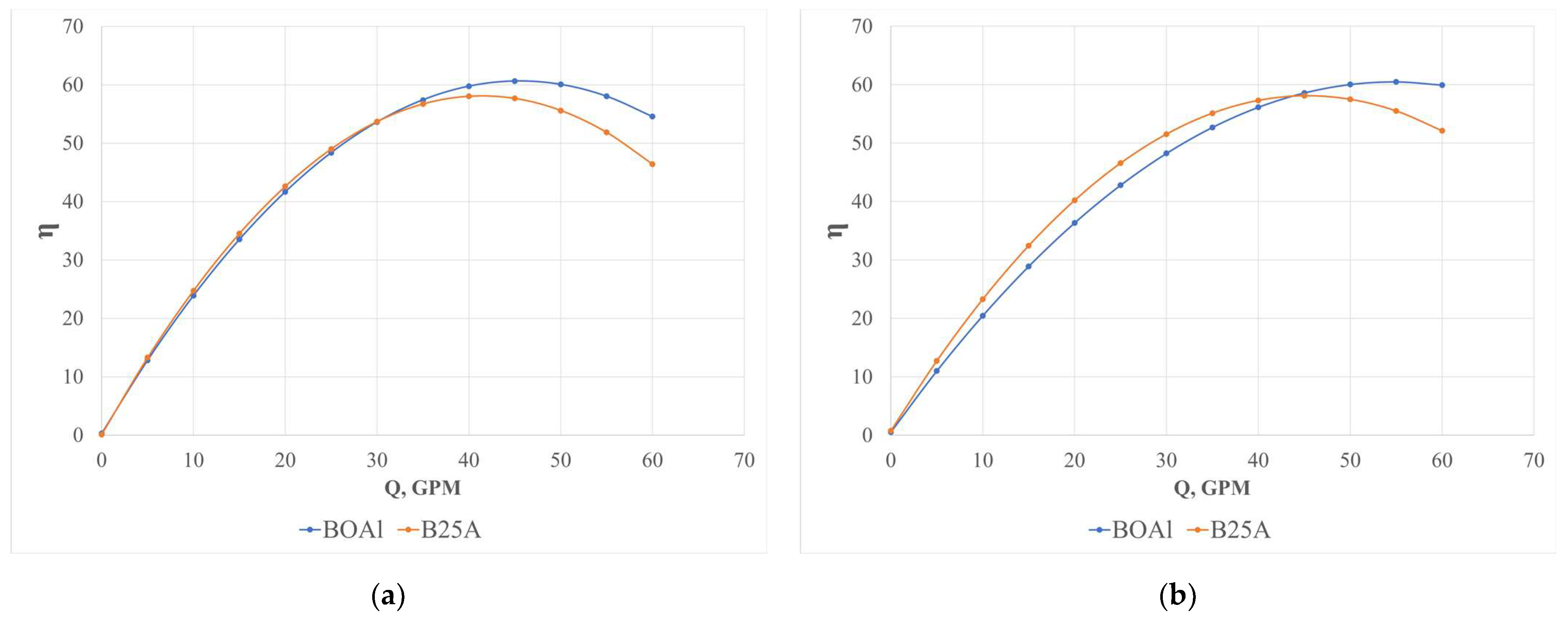
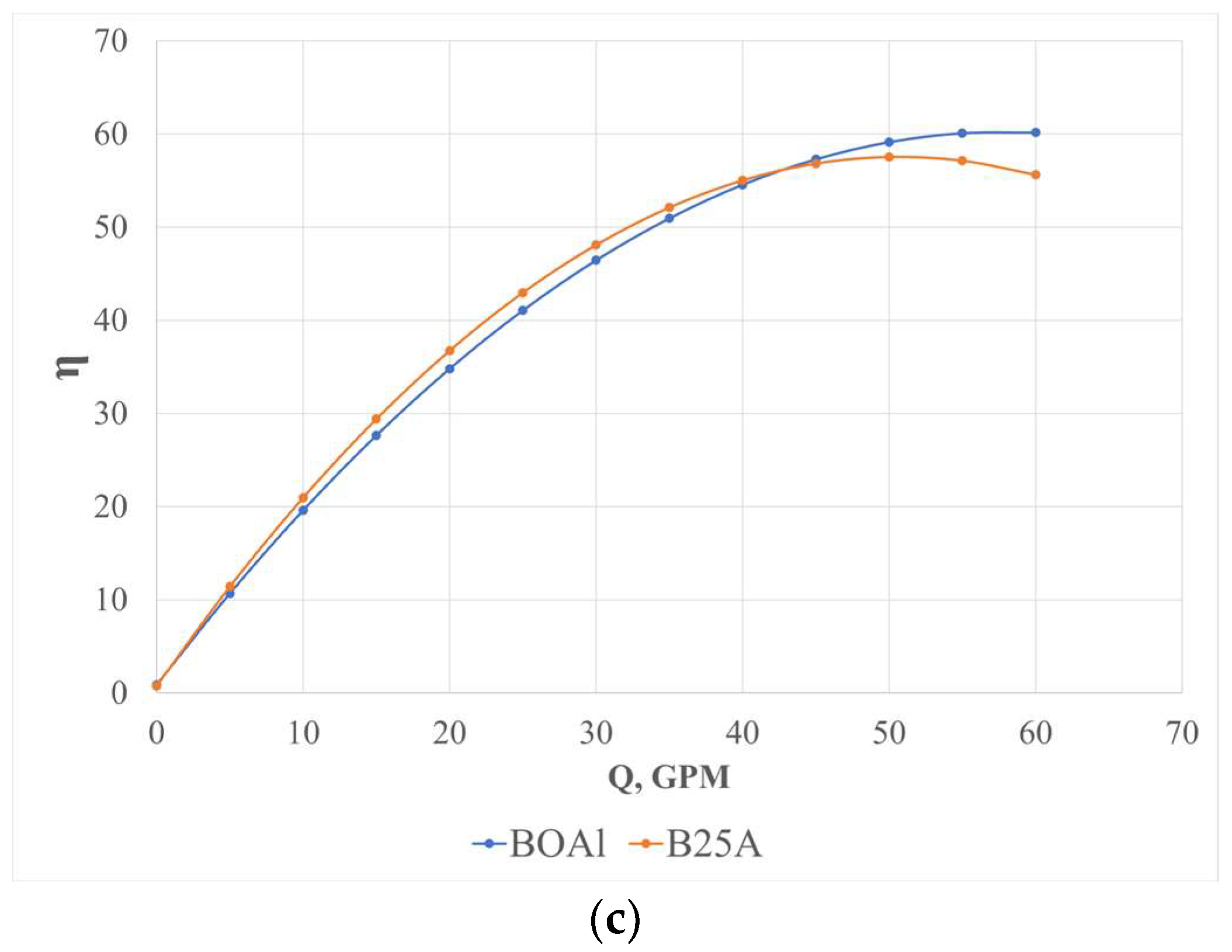
• Double curvature impellers at 25% of the length from the exterior diameter in relation to the interior diameter deliver more head than the original impeller; impeller B25A performed better compared to impeller B25B. This difference can be observed not only in the head–flow rate curve figures but also in the Turkey’s test. The performance of the pump–motor unit with impeller B25A was better than the original impeller.
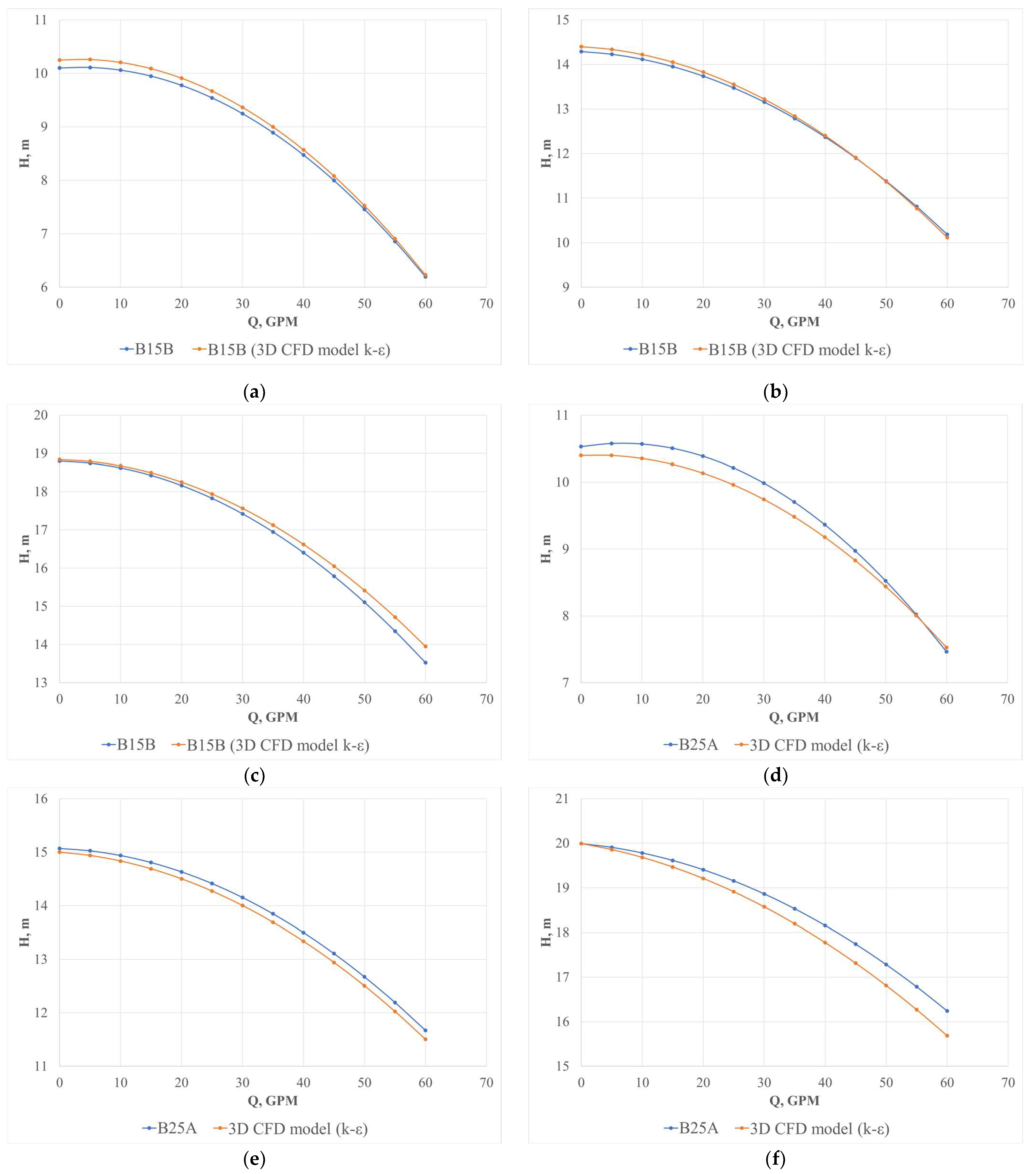
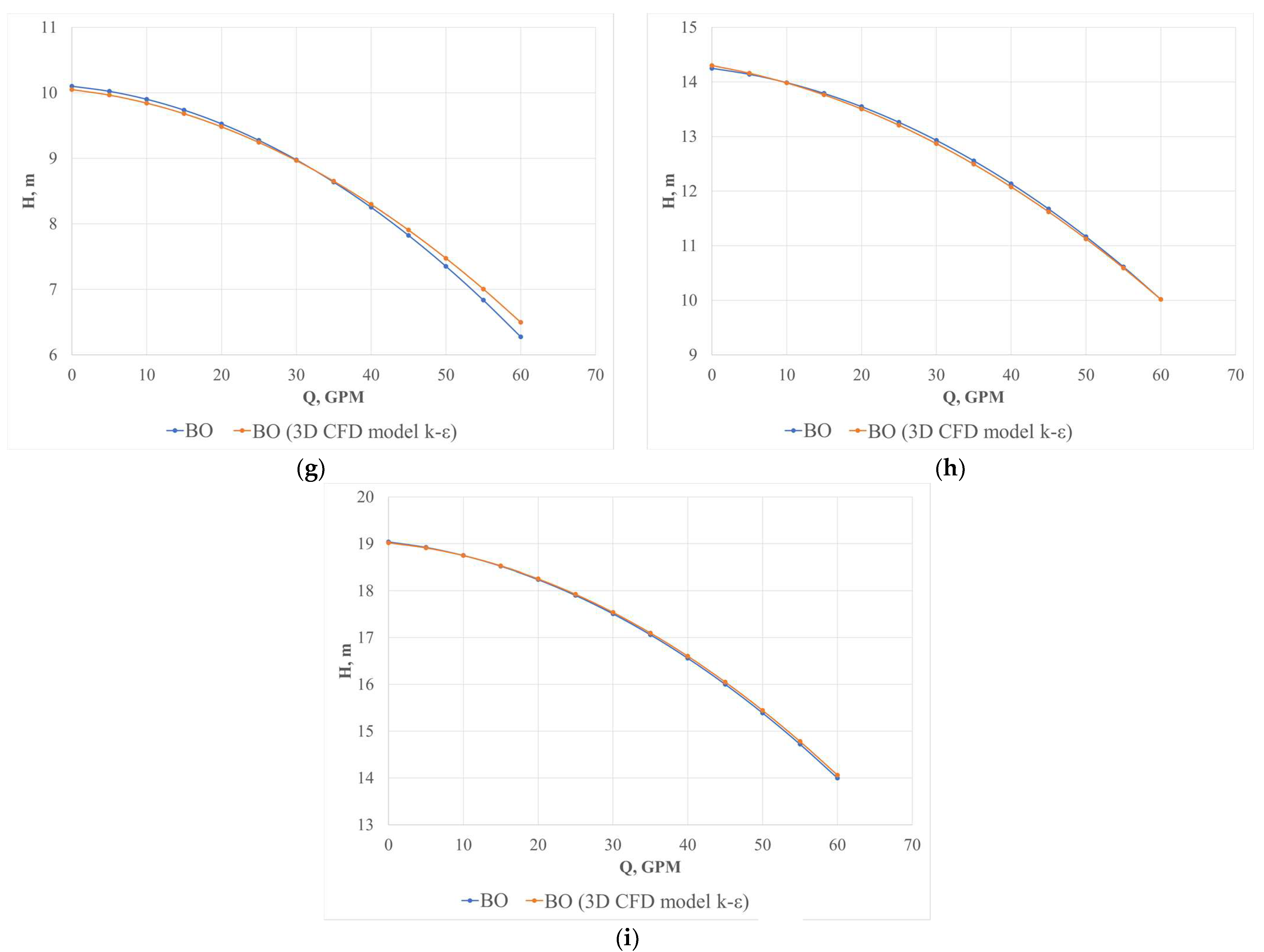
• The curves obtained experimentally and by simulation do not show a statistically significant difference with a 95% confidence interval.
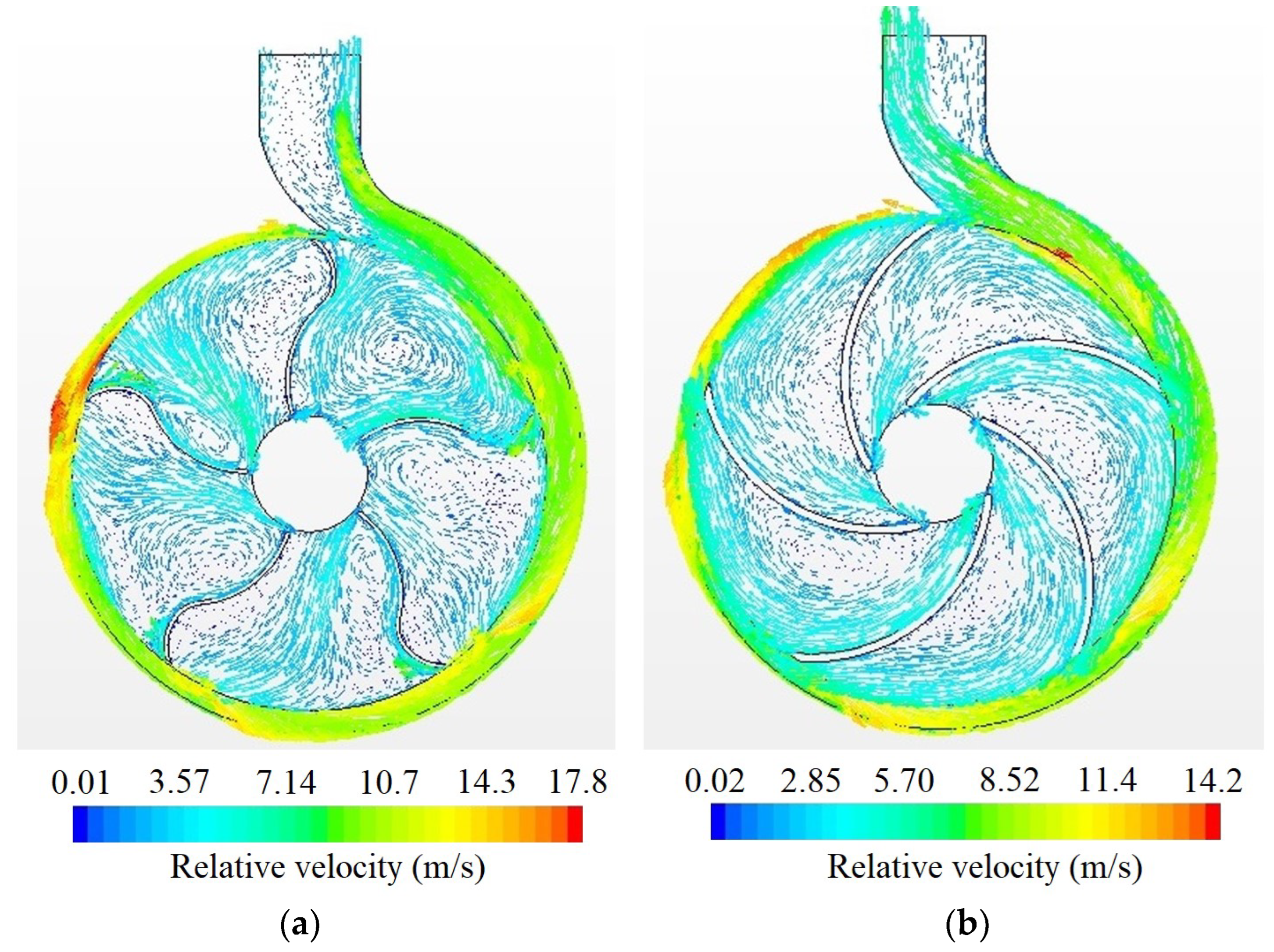
• For a better understanding of the physical behavior of variables such as pressure and flow velocity in the impellers and at the outlet of the pumping system, several three-dimensional CFD models were developed, which were used to represent the scenarios described in Table 1. In the different tests carried out, flows at the inlet and outlet were in the range of the Reynolds number between 10,304 and 138,951, being in the turbulent flow regime; therefore, the use of turbulence models was considered for the modelling of the pumping system.
• For the validation process, a mesh independence analysis and comparison with experimental pumping characteristic curves was performed, where the curves obtained from the CFD model showed a similar trend to the experimental curves.
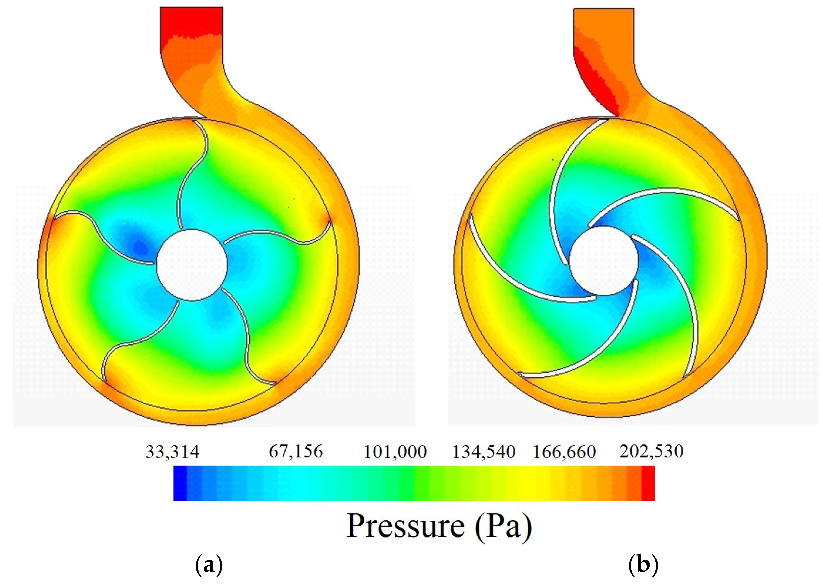
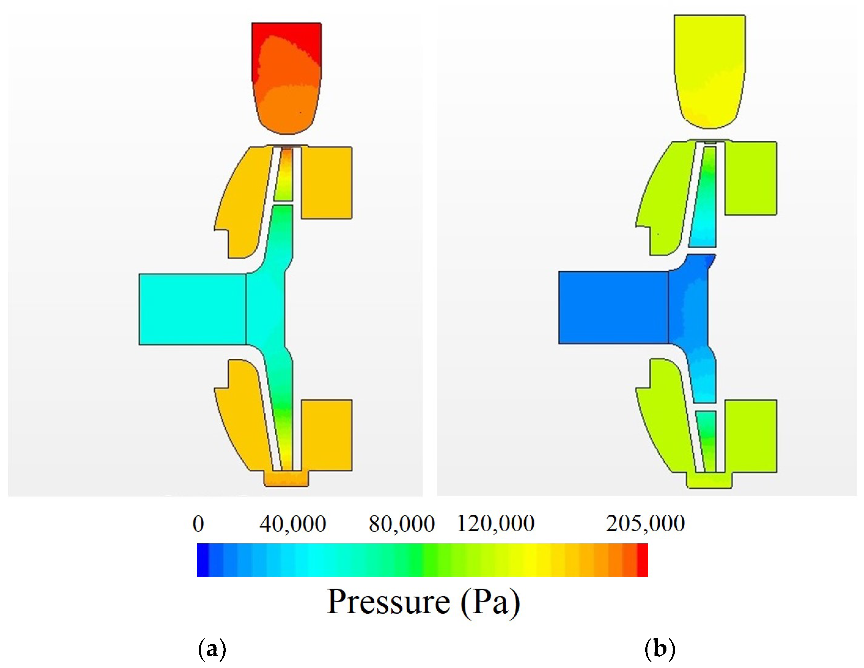
• It was identified, through CFD modelling, that the double curved blades generate higher pressure fronts when pushing the water towards the volute, leading to the generation of higher pressure compared to impellers without double curvature.
• The application of the k-ω SST and k-ε turbulence models was adequate to understand the physical behavior of the turbulence effects in impellers, where some numerical and spatial differences were identified concerning the generation of turbulent kinetic energy and the prediction of vorticity by summing the results of the velocity and pressure contours. However, it was found that the trend of the Q-H curves was similar using the different turbulence models. Finally, these turbulence models guarantee an adequate prediction of physical behavior concerning the Q-H ratio, and they have been used for similar analyses in previous research.

Pump manufacturers should explore double curvature impellers, since it is possible to increase the behavior of the head–flow rate curves compared to traditional designs. As a starting point, the authors recommend using the defined geometry for impeller B25A. This research presented head and performance pump curves considering double curvature impellers that can be used by manufacturers.

References

1. Patel, M.G.; Doshi, A.V. Effect of Impeller Blade Exit Angle on the Performance of Centrifugal Pump. Int. J. Emerg. Technol. Adv. Eng. 2013, 3, 702–706. [Google Scholar]
2. Tuzson, J. Centrifugal Pump Design; John Wiley & Sons, Inc.: Hoboken, NJ, USA, 2000. [Google Scholar]
3. Gulich, J.F. Centrifugal Pumps, 2nd ed.; Springer: New York, NY, USA, 2010. [Google Scholar]
4. Srinivasan, K. Rotodynamic Pumps (Centrifugal and Axial); New Age International (P) Ltd.: Delhi, India, 2008. [Google Scholar]
5. Spence, R.; Amaral-Teixeira, J. Investigation into pressure pulsations in a centrifugal pump using numerical methods supported by industrial tests. Comput. Fluids 2008, 37, 690–704. [Google Scholar] [CrossRef]
6. Spence, R.; Amaral-Teixeira, J. A CFD parametric study of geometrical variations on the pressure pulsations and performance characteristics of a centrifugal pump. Comput. Fluids 2009, 38, 1243–1257. [Google Scholar] [CrossRef] [Green Version]
7. Fontanals, A.; Guardo, A.; Coussirat, M.; Egusquiza, E. Numerical Study of the Fluid—Structure Interaction in the Diffuser Passage of a Centrifugal Pump. In Proceedings of the IV International Conference on Computational Methods for Coupled Problems in Science and Engineering, Kos, Greece, 20–22 June 2011. [Google Scholar]
8. Savar, M.; Kozmar, H.; Sutlović, I. Improving centrifugal pump efficiency by impeller trimming. Desalination 2009, 249, 654–659. [Google Scholar] [CrossRef]
9. Barrio, R.; Fern’andez, J.; Blanco, E.; Parrondo, J. Estimation of radial load in centrifugal pumps using computational fluid dynamics. Eur. J. Mech. B/Fluids 2011, 30, 316–324. [Google Scholar] [CrossRef]
10. Houlin, L.; Yong, W.; Shouqi, Y.; Minggao, T.A.N.; Kai, W. Effects of Blade Number on Characteristics of Centrifugal Pumps. Chin. J. Mech. Eng. 2010, 23, 742. [Google Scholar]
11. Li, W.-G. Influence of the Number of Impeller Blades on the Performance of Centrifugal Oil Pumps; World Pumps: Oxford, MS, USA, 2002. [Google Scholar]
12. Rababa, K.S. The Effect of Blades Number and Shape on the Operating Characteristics of Groundwater Centrifugal Pumps. Eur. J. Sci. Res. 2011, 52, 243–251. [Google Scholar]
13. Chakraborty, S.; Pandey, K.M. Numerical Studies on Effects of Blade Number Variations on Performance of Centrifugal Pumps at 4000 RPM. Int. J. Eng. Technol. 2011, 3, 410–416. [Google Scholar] [CrossRef] [Green Version]
14. Pandey, K.M.; Singh, A.P.; Chakraborty, S.; Engineering, M.; Silchar, N.I.T. Numerical studies on effects of blade number variations on performance of centrifugal pumps at 2500 RPM. J. Environ. Res. Dev. 2012, 6, 863–868. [Google Scholar]
15. Sanda, B.; Daniela, C.V. The Influence of the Inlet Angle Over the Radial Impeller Geometry Design Approach with ANSYS. J. Eng. Stud. Res. 2012, 18, 32–39. [Google Scholar] [CrossRef]
16. Luo, X.; Zhang, Y.; Peng, J.; Xu, H.; Yu, W. Impeller inlet geometry effect on performance improvement for centrifugal pumps. J. Mech. Sci. Technol. 2008, 22, 1971–1976. [Google Scholar] [CrossRef]
17. Shojaeefard, M.; Tahani, M.; Ehghaghi, M.; Fallahian, M.; Beglari, M. Numerical study of the effects of some geometric characteristics of a centrifugal pump impeller that pumps a viscous fluid. Comput. Fluids 2012, 60, 61–70. [Google Scholar] [CrossRef]
18. Bacharoudis, E.C.; Filios, A.E.; Mentzos, M.D.; Margaris, D.P. Parametric Study of a Centrifugal Pump Impeller by Varying the Outlet Blade Angle. Open Mech. Eng. J. 2008, 2, 75–83. [Google Scholar] [CrossRef]
19. Al-Qutub, A.M.; Khalifa, A.E.; Al-Sulaiman, F.A. Exploring the Effect of V-Shaped Cut at Blade Exit of a Double Volute Centrifugal Pump. J. Press. Vessel. Technol. 2012, 134, 8. [Google Scholar] [CrossRef]
20. Patil, P.M.; Patil, S.S.; Todkar, R.G. Design, Development and Testing of an Impeller of Open Well Submersible Pump for Performance Improvement. Int. J. Sci. Res. 2014, 3, 2670–2675. [Google Scholar]
21. Anagnostopoulos, J.S. A fast numerical method for flow analysis and blade design in centrifugal pump impellers. Comput. Fluids 2009, 38, 284–289. [Google Scholar] [CrossRef]
22. Grapsas, V.A.; Anagnostopoulos, J.S.; Papantonis, D.E. Experimental and Numerical Study of a radial Flow Pump Impeller with 2D-Curved Blades. In Proceedings of the International Conference on Fluid Mechanics and Aerodynamics, Athens, Greece, 25–27 August 2007; pp. 175–180. [Google Scholar]
23. Zhou, W.; Zhao, Z.; Lee, T.S.; Winoto, S.H. Investigation of Flow Through Centrifugal Pump Impellers Using Computational Fluid Dynamics. Int. J. Rotating Mach. 2003, 9, 49–61. [Google Scholar] [CrossRef] [Green Version]
24. Yang, M.G.; Liu, D.; Gu, H.F.; Kang, C.; Li, H. Analysis of Turbulent Flow in the Impeller of a Chemical Pump. J. Eng. Sci. Technol. 2007, 2, 218–225. [Google Scholar]
25. Shvindin, A.I.; Ivanyushin, A.A. Operation of centrifugal pumps in off-design conditions. Chem. Pet. Eng. 2009, 45, 148–151. [Google Scholar] [CrossRef]
26. Cheah, K.W.; Lee, T.S.; Winoto, S.H.; Zhao, Z.M. Numerical Flow Simulation in a Centrifugal Pump at Design and Off-Design Conditions. Int. J. Rotating Mach. 2007, 2007, 083641. [Google Scholar] [CrossRef]
27. Barrio, R.; Parrondo, J.; Blanco, E. Numerical analysis of the unsteady flow in the near-tongue region in a volute-type centrifugal pump for different operating points. Comput. Fluids 2010, 39, 859–870. [Google Scholar] [CrossRef]
28. Ozturk, A.; Aydin, K.; Sahin, B.; Pinarbasi, A. Effect of impeller-diffuser radial gap ratio in a centrifugal pump. JSIR 2009, 68, 203–213. [Google Scholar]
29. Gupta, M.; Kumar, S.; Kumar, A. Numerical Study of Pressure and Velocity Distribution Analysis of Centrifugal Pump. Int. J. Therm. Technol. 2011, 1, 114–118. [Google Scholar]
30. Asuaje, M.; Bakir, F.; Kouidri, S.; Kenyery, F.; Rey, R. Numerical Modelization of the Flow in Centrifugal Pump: Volute Influence in Velocity and Pressure Fields. Int. J. Rotating Mach. 2005, 2005, 244–255. [Google Scholar] [CrossRef] [Green Version]
31. Esfahani, J.A.; Moghadam, B.J.; Nouri, M.; Mahmoudi, A. Numerical and parametric study of a centrifugal pump. In Proceedings of the International Conference on Advances in Mechanical and Robotics Engineering—MRE 2014, Kuala Lumpur, Malaysia, 8–9 March 2014; pp. 35–39. [Google Scholar]
32. Kulkarni, S.S. Parametric Study of Centrifugal Pump and its Performance Analysis using CFD. Int. J. Emerg. Technol. Adv. Eng. 2014, 4, 155–161. [Google Scholar]
33. Shojaeefard, M.H.; Boyaghchi, F.A.; Ehghaghi, M.B. Experimental Study and Three-Dimensional Numerical Flow Simulation in a Centrifugal Pump when Handling Viscous Fluids. IUST Int. J. Eng. Sci. 2006, 17, 53–60. [Google Scholar]
34. Fard, M.H.S.; Boyaghchi, F.A. Studies on the Influence of Various Blade Outlet Angles in a Centrifugal Pump when Handling Viscous Fluids. Am. J. Appl. Sci. 2007, 4, 718. [Google Scholar] [CrossRef]
35. Pagalthivarthi, K.V.; Gupta, P.K.; Tyagi, V.; Ravi, M.R. CFD Predictions of Dense Slurry Flow in Centrifugal Pump Casings. Int. J. Aerosp. Mech. Eng. 2011, 5, 254–266. [Google Scholar]
36. Gölcü, M.; Pancar, Y. Investigation of Performance Characteristics in a Pump Impeller with Low Blade Discharge Angle; World Pumps: Oxford, MS, USA, 2005. [Google Scholar]
37. Baoling, C.; Zuchao, Z.; Jianci, Z.; Ying, C. The Flow Simulation and Experimental Study of Low Specific-Speed High-speed Complex Centrifugal Impellers. Chin. J. Mech. Eng. 2006, 14, 435–441. [Google Scholar]
38. Kaya, D.; Yagmur, E.A.; Yigit, K.S.; Kilic, F.C.; Eren, A.S.; Celik, C. Energy efficiency in pumps. Energy Convers. Manag. 2008, 49, 1662–1673. [Google Scholar] [CrossRef]
39. Yedidiah, S. A Study in the Use of CFD in the Design of Centrifugal Pumps. Eng. Appl. Comput. Fluid Mech. 2008, 2, 331–343. [Google Scholar] [CrossRef] [Green Version]
40. Wu, K.-H.; Lin, B.-J.; Hung, C.-I. Novel Design of Centrifugal Pump Impellers Using Generated Machining Method and CFD. Eng. Appl. Comput. Fluid Mech. 2008, 2, 195–207. [Google Scholar] [CrossRef] [Green Version]
41. Bachus, L. ADHD and NPSH; World Pumps: Oxford, MS, USA, 2005; pp. 26–29. [Google Scholar]
42. Abbas, M.K. Cavitation in centrifugal pumps. Diyala J. Eng. Sci. 2010, 170–180. [Google Scholar]
43. Černetič, J.; Čudina, M. Cavitation Noise Phenomena in Centrifugal Pumps. In Proceedings of the 5th Congress of Alps-Adria Acoustics Association, Petrcane, Croatia, 12–14 September 2012; pp. 1–6. [Google Scholar]
44. Budea, S.; Ciocanea, A. The Influence of the Suction Vortex Over the NPSH Available of Centrifugal Pumps. U.P.B. Sci. Bull. 2008, 70, 1–10. [Google Scholar]
45. Shah, S.R.; Jain, S.V.; Patel, R.N.; Lakhera, V.J. CFD for centrifugal pumps: A review of the state-of-the-art. Procedia Eng. 2013, 51, 715–720. [Google Scholar] [CrossRef] [Green Version]
46. Cherkasski, V. Pumps, Fans, Compressors; MIRED: Moscow, Russia, 1980. [Google Scholar]
47. Ke, Q.; Tang, L.; Luo, W.; Cao, J. Parameter Optimization of Centrifugal Pump Splitter Blades with Artificial Fish Swarm Algorithm. Water 2023, 15, 1806. [Google Scholar] [CrossRef]
48. Hu, J.; Li, K.; Su, W.; Zhao, X. Numerical Simulation of Drilling Fluid Flow in Centrifugal Pumps. Water 2023, 15, 992. [Google Scholar] [CrossRef]
49. PTC 8.2-1990; Centrifugal Pumps. ASME: New York, NY, USA, 1990.
50. Greenshields, C.; Weller, H. Notes on Computational Fluid Dynamics: General Principles; CFD Direct Ltd.: Reading, UK, 2022. [Google Scholar]
51. Launder, B.E.; Spalding, D.B. The Numerical Computation of Turbulent Flows. In Numerical Prediction of Flow, Heat Transfer, Turbulence and Combustion; Imperial College of Science and Technology, Department of Mechanical Engineering; Elsevier: London, UK, 1983; pp. 96–116. [Google Scholar]
52. Liu, H.L.; Liu, M.M.; Dong, L.; Ren, Y.; Du, H. Effects of computational grids and turbulence models on numerical simulation of centrifugal pump with CFD. IOP Conf. Ser. Earth Environ. Sci. 2012, 15, 062005. [Google Scholar] [CrossRef]
53. Menter, F.R. Two-equation eddy-viscosity turbulence models for engineering applications. AIAA J. 1994, 32, 1598–1605. [Google Scholar] [CrossRef] [Green Version]
54. Menter, F.R. Review of the shear-stress transport turbulence model experience from an industrial perspective. Int. J. Comput. Fluid Dyn. 2009, 23, 305–316. [Google Scholar] [CrossRef]
55. Kaewnai, S.; Chamaoot, M.; Wongwises, S. Predicting performance of radial flow type impeller of centrifugal pump using CFD. J. Mech. Sci. Technol. 2009, 23, 1620–1627. [Google Scholar] [CrossRef]
56. Chima, R.; Liou, M.S. Comparison of the AUSM+ and H-CUSP Schemes for Turbomachinery Applications. In Proceedings of the 16th AIAA Computational Fluid Dynamics Conference, Orlando, FL, USA, 23–26 June 2003; p. 4120. [Google Scholar]
57. Wu, J.; Shimmei, K.; Tani, K.; Niikura, K.; Sato, J. CFD-based design optimization for hydro turbines. J. Fluids Eng. 2007, 129, 159–168. [Google Scholar] [CrossRef]
58. Mott, R.L. Applied Fluid Mechanics, 6th ed.; Pearson Education: London, UK, 2016. [Google Scholar]
59. Montgomery, D.C. Design and Analysis of Experiments, 8th ed.; LWW: Philadelphia, PA, USA, 2012. [Google Scholar]
Figure 1. Schematic diagram of experimental facility.
Fluids 08 00217 g001
Figure 2. Configurations of impellers: (a) Original bronze (BO) and aluminum (BOAI) impeller; and (b) double curvature impellers.
Fluids 08 00217 g002
Figure 3. Details of geometry representation: (a) geometry of CFD model with its boundaries; (b) details of mesh in Rotating Fluid and interfaces; (c) mesh of the section view of impeller and discharge; and (d) an example of an impeller used in the laboratory.
Fluids 08 00217 g003
Figure 4. 3D Mesh of fluid domain for simulation of pumping system (Fluid Region), with details in wall near zone.
Fluids 08 00217 g004
Figure 5. Characteristics of meshes used for independence analysis: (a) illustration of different meshes and details, (b) variation of difference in pressure between admission and discharge for three meshes, and (c) results of velocities at admission and discharge for different meshes.
Fluids 08 00217 g005
Figure 6. Head–flow rate curve for impellers: (a) BO and BOAl at 1400 RPM; (b) BO and BOAl at 1700 RPM; (c) BO and BOAl at 1900 RPM; (d) B25A, B25B, B50A, B50B, and B15B at 1400 RPM; (e) B25A, B25B, B50A, B50B, and B15B at 1700 RPM; (f) B25A, B25B, B50A, B50B, and B15B at 1900 RPM.
Fluids 08 00217 g006
Figure 7. Performance–flow rate curve of the pump–motor unit for impellers: (a) BO and BOAl at 1400 RPM; (b) BO and BOAl at 1700 RPM; (c) BO and BOAl at 1900 RPM; (d) B25A, B25B, B50A, B50B, and B15B at 1400 RPM; (e) B25A, B25B, B50A, B50B, and B15B at 1700 RPM; (f) B25A, B25B, B50A, B50B, and B15B at 1900 RPM.
Fluids 08 00217 g007
Figure 8. Head–flow rate Tukey’s test for impellers: (a) BO and BOAl at 1400 RPM; (b) BO and BOAl at 1700 RPM; (c) BO and BOAl at 1900 RPM; (d) B25A, B25B, B50A, B50B, and B15B at 1400 RPM; (e) B25A, B25B, B50A, B50B, and B15B at 1700 RPM; (f) B25A, B25B, B50A, B50B, and B15B at 1900 RPM.
Fluids 08 00217 g008aFluids 08 00217 g008b
Figure 9. Head–flow rate calculation by simulation for impellers BO and B25A at: (a) 1400 RPM; (b) 1700 RPM; (c) 1900 RPM.
Fluids 08 00217 g009aFluids 08 00217 g009b
Figure 10. Head–flow rate; Tukey’s test for impellers BO and B25A: (a) 1400 RPM; (b) 1700 RPM; (c) 1900 RPM.
Fluids 08 00217 g010
Figure 11. Performance–flow rate Tukey’s test for impellers at: (a) 1400 RPM; (b) 1700 RPM; and (c) 1900 RPM.
Fluids 08 00217 g011
Figure 12. Performance–flow rate curve for impellers BOAl and B25A at: (a) 1400 RPM; (b) 1700 RPM; (c) 1900 RPM.
Fluids 08 00217 g012aFluids 08 00217 g012b
Figure 13. Pressure distribution in pump interior using impellers at 1700 RPM: (a) B25A impeller; and (b) BO impeller.
Fluids 08 00217 g013
Figure 14. Pressure distribution in the pump interior when transitioning from suction to outlet at 1700 RPM: (a) B25A impeller; and (b) BO impeller.
Fluids 08 00217 g014
Figure 15. Relative velocity vectors at 1700 RPM: (a) B25A impeller; and (b) BO impeller.
Fluids 08 00217 g015
Figure 16. Comparison between experimental versus CFD results: (a) B15B at 1400 RPM; (b) B15B at 1700 RPM; (c) B15B at 1900 RPM; (d) B25A at 1400 RPM; (e) B25A at 1700 RPM; (f) B25A at 1900 RPM; (g) BO at 1400 RPM; (h) BO at 1700 RPM; (i) BO at 1900 RPM.
Fluids 08 00217 g016aFluids 08 00217 g016b
Figure 17. Comparison of turbulence models using CFD results: (a) B25A at 1400 RPM; (b) B25A at 1700 RPM; and (c) B125A at 1900 RPM.
Fluids 08 00217 g017
Figure 18. Comparison of pressure contours of impeller B25A using a velocity of 1700 RPM: (a) k-ε, and (b) SST k-ω turbulence model.
Fluids 08 00217 g018
Figure 19. Comparison of relative velocity contours of impeller B25A using a velocity of 1700 RPM: (a) k-ε, and (b) SST k-ω turbulence model.
Fluids 08 00217 g019
Figure 20. Comparison of contours of turbulent kinetic energy of impeller B25A using a velocity of 1700 RPM: (a) k-ε, and (b) SST k-ω turbulence model.
Fluids 08 00217 g020
Figure 21. Comparison of vorticity contours of impeller B25A using a velocity of 1700 RPM: (a) k-ε, and (b) SST k-ω turbulence model.
Fluids 08 00217 g021