Abstract
Traditionally, Fourier spectra have been employed to gain a deeper understanding of turbulence flow structures. The investigation of isotropic forced turbulence with passive scalars offers a straightforward means to examine the disparities between velocity and passive scalar spectra. This flow configuration has been extensively studied in the past, encompassing a range of Reynolds and Schmidt numbers. In this present study, direct numerical simulations (DNS) of this flow are conducted at sufficiently high Reynolds numbers, enabling the formation of a wide inertial range. The primary focus of this investigation is to quantitatively assess the variations in scalar spectra with the Schmidt number (Sc). The spectra exhibit a transition from a k−5/3 scaling for low Sc to a k−4/3 scaling for high Sc. The emergence of the latter power law becomes evident at Sc = 2, with its width expanding as Sc increases. To gain further insights into the underlying flow structures, a statistical analysis is performed by evaluating quantities aligned with the principal axes of the strain field. The study reveals that enstrophy is primarily influenced by the vorticity aligned with the intermediate principal strain axis, while the scalar gradient variance is predominantly controlled by the compressive strain. To provide a clearer understanding of the differences between enstrophy and scalar gradient variance, joint probability density functions (PDFs) and visualizations of the budget terms for both quantities are presented. These visualizations serve to elucidate the distinctions between the two and offer insights into their respective behaviors.
1. Introduction
The Schmidt number is a dimensionless quantity that characterizes the relative importance of momentum diffusion to the diffusivity of passive scalars, namely . It is particularly relevant when dealing with the transport of passive scalars, such as temperature, concentration, or other non-momentum-transporting properties, in a turbulent flow. In forced isotropic turbulence, external energy is continuously injected into the system to maintain turbulence. Passive scalars in this context refer to quantities that do not actively contribute to the turbulent energy generation but are instead transported by the turbulent flow. The effect of the Schmidt number on forced isotropic turbulence with passive scalars strongly impacts several physical processes. At low Schmidt number () molecular diffusivity is high compared to the turbulent mixing. In this case, passive scalars are mixed efficiently, and their gradients are rapidly flattened due to the dominant influence of molecular diffusion. As a result, sharp gradients in the scalar field are quickly smoothed out. At higher Schmidt numbers (), molecular diffusion becomes less significant compared to turbulent mixing. This allows for concentration fluctuations to persist over longer-length scales before being smoothed out by diffusion. Consequently, the scalar field might exhibit more complex and smaller-scale structures. The scalar dissipation rate, which quantifies how quickly the scalar variance is dissipated, is affected by the Schmidt number, as lower Schmidt numbers generally result in higher scalar dissipation rates due to the dominance of diffusion, whereas higher Schmidt numbers lead to lower scalar dissipation rates due to enhanced mixing.
Direct numerical simulations (DNS) have long been employed as a powerful tool for investigating the intricate dynamics of passive scalars advected by turbulent flows. In the context of studying these phenomena, isotropic turbulence has often been simulated using DNS with a low wavenumber forcing. This setup enables the attainment of statistically stationary states within a few eddy turnover times, facilitating the collection of extensive datasets for an in-depth analysis of high-order statistical properties. It is worth noting that the extensive body of literature on forced isotropic turbulence with and without passive scalars makes it impractical to provide a comprehensive list of relevant papers in this brief discussion. However, the review by Ishihara et al. [1] provides a comprehensive compilation of papers on forced isotropic turbulence without passive scalars, while Donzis et al. [2] catalog the studies specifically focused on passive scalars, shedding light on the differences and similarities between velocity and passive scalar statistics, including their spectral properties. An alternative approach to studying passive scalars in turbulent flows involves DNS of decaying turbulence, initiated with prescribed spectra and random phases. Although this method deviates from realistic initial conditions, it provides insights into the effects of varying parameters, such as the Schmidt number. Orlandi and Antonia [3] conducted a study specifically focused on understanding the influence of Schmidt number variations on the decay of passive scalars. They compared DNS results with those obtained using eddy-damped quasi-normal Markovian (EDQNM) closures, which offer information about high Reynolds number regimes that would otherwise require computationally prohibitive efforts to achieve with DNS. By leveraging DNS and incorporating spectral closures, researchers have been able to delve into the complex dynamics of passive scalars in turbulent flows, exploring a wide range of scenarios and parameters. The combination of these techniques allows for a comprehensive investigation of the complex physics underlying the behavior of passive scalars, providing insights that contribute to our understanding of turbulent transport processes.
In a distinct approach, Orlandi et al. [4] employed a minimal flow unit (MFU) framework to investigate various aspects of isotropic turbulence and the turbulent transport of passive scalars. They initiated their simulations by introducing two orthogonal Lamb dipoles, allowing them to interact and evolve. Initially, the flow exhibited a vortical-dominated stage where vortex structures of smaller scales were generated through vortex stretching. During the initial phase, the number and shape of the vortex structures generated from the initial conditions were similar to those generated under inviscid conditions. However, as the simulation progressed and approached the time of the finite-time singularity, the vortical structures in the viscous case became dependent on the viscosity. The statistical properties, including the velocity and passive scalar spectra, coincided with those observed in forced isotropic turbulence.
The utilization of the MFU framework provided a detailed analysis of the dynamics of the components of the vorticity and scalar gradient vectors along with the principal axes of the strain rate tensor. These analyses corroborated the findings reported by Tsinober [5] regarding the importance of the intermediate strain in the evolution of enstrophy and the compressive strain in the scalar gradient variance. Additionally, flow visualizations were presented to enhance the understanding of the underlying physics. Notably, Orlandi et al. [4] limited their simulations to a passive scalar with unit Schmidt number.
Through the implementation of the MFU framework, Orlandi et al. [4] provided a comprehensive examination of the complex dynamics and statistical properties of isotropic turbulence and passive scalar transport. Their work shed light on the behavior of vortical structures and their relationship with viscosity, as well as the crucial roles played by different strain components in the evolution of enstrophy and scalar gradient variance.
In the present paper, simulations of forced turbulence were conducted at both high and low Reynolds numbers to investigate the transport of passive scalars, at various Schmidt numbers. Two different forcing methods were employed for the passive scalar, one similar to that used for the velocity field to maintain a constant passive scalar variance during the evolution towards the statistical steady state, and the other method employed by Donzis et al. [2]. The choice of forcing method had an impact on the dynamics, leading to oscillations in the scalar dissipation. The simulations using the second forcing method exhibited growing oscillations, rendering them unsuitable for analyzing the spectra and the terms in the balance equations of enstrophy and scalar gradient variance.
One unresolved question is whether the scalar spectrum, at any Schmidt number, exhibits an inertial range with a power-law decay of similar to the kinetic energy spectrum, or maybe other decay laws. In this respect, Lohse [6] argued that in sheared turbulence, passive scalars should have a spectral range. In fact, based on the assumption that in shear-dominated turbulence, the velocity spectrum should display a spectral range [7], the respective Fourier coefficients should scale as . Assuming the constancy of the passive scalar flux in wavenumber space, (with the scalar dissipation rate), it readily follows that . Support for this scaling law came from measurements of temperature fluctuations in the wake of a heated cylinder [8]. A theory for the behavior of scalar spectra in stratified turbulence was proposed by Bolgiano [9] and Obukhov [10]. In analogy with Kolmogorov’s theory, and assuming that next to a given flow scale k, the only relevant parameters are the thermal dissipation rate and the product of the thermal expansion coefficient and gravity, a dimensional analysis readily yield the prediction , which is commonly referred to as the Bolgiano–Obukhov scaling. Numerical experiments by Camussi and Verzicco [11] in cylindrical cells supported the reduced decay predicted by the Bolgiano–Obukhov scaling, as shown in Figure 5 of Lohse and Xia [12]. Orlandi and Pirozzoli [13] carried out DNS of natural convection at high Rayleigh numbers and a Prandtl number and observed a wide power-law spectral range with an exponent close to either or .
To explore the dependence of the decay exponent on the Schmidt number and shed light on the differences in the dynamics of enstrophy and scalar gradient variance, DNS of forced isotropic turbulence transporting passive scalars at various was conducted in this study. These simulations provide information about the Schmidt number dependence of the decay exponent and contribute to understanding the distinct behaviors of enstrophy and scalar gradient variance.
2. Relevant Equations
The momentum and continuity equations for incompressible flows are as follows
where are the components of the velocity vector in the i directions, p is the pressure, , , and are the three orthogonal space directions, and is the external forcing to prevent decay of the turbulence kinetic energy . The passive scalar is transported by the velocity field according to
where is introduced to prevent a decay of the passive scalar variance, . The numerical simulations are initiated with velocity and scalar fields with random phases, representing flows without structures but with high energy at low wavenumbers and small energy at large wavenumbers. The initial kinetic energy spectrum is given by the equation , with , and . The reference velocity is , and the Taylor Reynolds number (later defined) is related to the initial spectrum through
The value of is determined by assigning a value to , as well as specifying the values of . The same spectrum is used to generate the initial distribution of the passive scalar field . The velocity components and the passive scalar in physical space are obtained using the method described by Rogallo [14].
The velocity components and the passive scalar in wavenumber space are given by
where the hat symbol is used to denote complex quantities. This expression satisfies the condition for a divergence-free velocity field in wavenumber space. Additionally, it can be demonstrated that if the following expressions are satisfied
the three-dimensional energy spectrum of the velocity field matches the given spectrum. To distribute the angles , and uniformly over the interval , four sets of random numbers are used. By applying the fast Fourier transform (FFT), the initial velocity and thermal fields in physical space are obtained.
To achieve a statistically steady state in the transport equations, forcing terms are introduced. Various forcing methods were discussed by Eswaran and Pope [15], based on the concept that at high Reynolds numbers, the dynamics of the small scales should be decoupled from the large scales. However, manipulating the large scales can impact the rate of energy dissipation. A statistical steady state is reached when the dissipation rate oscillates around a constant value over time. Without forcing, the root mean square velocity , at each instant, has a total energy component , that is less than the initial energy . By selecting a threshold wavenumber , the energy within the range is evaluated to determine the quantity , which represents the proportion of energy lost. By modifying the components for through , the total energy can be kept constant over time. In the simulations described in this paper, a numerical scheme was employed in physical space, and thus three-dimensional FFT operations were used to transition between physical and wavenumber spaces. Within the wavenumber space, the components were modified for . Subsequently, an inverse three-dimensional FFT was applied to obtain the modified velocity in physical space. To save computational time, the forcing was only applied during the last of the three Runge–Kutta steps used for time advancement. The same forcing approach was also employed in the solution of the passive scalar transport equation, resulting in a constant , throughout the time evolution.
In contrast to the forcing scheme just described, Donzis et al. [2] used a forcing term for Equation (2), of the type , mimicking the effect of a mean passive scalar gradient as found in natural convection flow. They assumed a constant gradient . In this scenario, not only does the rate of scalar dissipation vary over time, but the quantity also experiences temporal fluctuations. Both forcing methods, as described by Eswaran and Pope [15] and Donzis et al. [2], were utilized in the present paper, and their respective results are discussed later on.
The system of equations given by (1) and (2), subject to periodic boundary conditions in the Cartesian directions , was numerically solved using a finite difference scheme as described in Orlandi [16]. To handle the temporal integration, an implicit Crank–Nicholson scheme was employed for the viscous terms, while a third-order Runge–Kutta scheme was utilized for the convective terms. By adopting a staggered arrangement of the velocity components, any odd–even decoupling phenomena were effectively eliminated, ensuring the discrete conservation of the total kinetic energy in the inviscid limit. The nondimensional temperature was placed at the same location as , which proves particularly advantageous in the presence of mean stratification, as it preserves the sum of potential and kinetic energy. To facilitate the implementation of MPI (message passing interface) coding, the computational domain was divided into layers parallel to the direction.
3. Results
3.1. Global Flow Parameters and Validation
Numerical simulations were performed at several Reynolds and Schmidt numbers, with an appropriate resolution chosen to ensure the maximum resolved wavenumber , where the superscript * indicates a normalization in Kolmogorov units. The following definitions are required to obtain this normalization from nondimensional computational units
The energy spectra in Kolmogorov units were obtained by scaling the velocity energy spectrum by , which represents the normalization factor for energy. Similarly, the root-mean-square (rms) velocity was obtained by dividing the square root of the velocity variances in computational units by , the normalization factor for velocity. The scalar energy spectrum was scaled by , while the passive scalar rms was normalized by .
The global data for the relevant simulations regarding the velocity are presented in Table 1, and the data for the passive scalar are reported in Table 2. The results presented in Table 1 demonstrate that a series of simulations with an grid resolution achieve a sufficiently high Taylor Reynolds number () to capture a power-law inertial range characterized by a scaling. Moreover, the maximum resolved wavenumber indicates that the simulations effectively resolve the exponential decay range of the spectrum. Simulations with an resolution were also conducted, employing the same random forcing as the cases. The influence of the passive scalar forcing was investigated using two different forcing methods as previously mentioned. The simulations at aimed to study the effect of high Schmidt numbers () on the passive scalar spectra. In Table 2, the global quantities related to the passive scalar are denoted by the same letter as in Table 1, with an additional index corresponding to the specific value of the Schmidt number.

Table 1.
Global quantities related to the solution of Equation (1).
Table 2.
Global quantities related to the solution of Equation (2), including the Schmidt number (), Batchelor length scale (), and normalization factors for the scalar energy spectrum (), and for the passive scalar rms (), passive scalar variance (), the integrated scalar spectrum dissipation (), and the scalar gradient dissipation rate ().
The simulations conducted in this study exhibit a linear growth of the dissipation rate with respect to the Reynolds number (), approximately given by . Consequently, the energy dissipation rate remains nearly independent of the Reynolds number. A similar linear growth of with was observed in the interaction of two orthogonal Lamb dipoles by Orlandi et al. [4]. In that case, without any external forcing, increased over time at a rate dependent on and eventually reached the same value at a certain nondimensional time. Subsequently, decreased over time independently of the Reynolds number. In the present simulations, the forcing was employed to achieve a statistical steady state within a certain number of eddy turnover times. This transient phase involved the formation of turbulent structures that were absent at the initial time. Depending on the specific forcing method employed, the energy may remain constant during this transient phase, while significant variations in and can occur. At a certain point in the simulations, the statistical quantities started to exhibit oscillations. From this point onward, time averages were computed to obtain the mean values of and , which are presented in Table 1. Additionally, the effect of the forcing method on the spectra was investigated, and comparisons were made with pseudospectral simulations available in the literature.
To validate the accuracy of the present second-order finite difference scheme and examine the spectra, comparisons were made with the results from the pseudospectral simulations conducted by Jiménez et al. [17]. The pseudospectral simulations considered various values of the Taylor Reynolds number, with the highest reported at . In the simulations by Jiménez et al. [17], the forcing at wavenumbers was implemented by assuming a negative viscosity coefficient of appropriate magnitude, adjusted periodically to maintain . In the simulations conducted by Donzis et al. [2] at , the forcing in the momentum equation was implemented by fixing the spectrum for wavenumbers , based on prior simulations that utilized a stochastic forcing scheme. With this type of forcing, the total energy varies over time, and the spectrum at low wavenumbers appears relatively smooth. In contrast, in the present simulations, the total energy was kept constant, resulting in oscillations in the spectra at low wavenumbers. Figure 1 compares the spectra of cases A, B, and C with those from the simulations of Jiménez et al. [17] and Donzis et al. [2]. The longitudinal and transverse one-dimensional spectra (Figure 1a and Figure 1b, respectively) highlight the effects of the forcing method. In wavenumber space, the simulations exhibit a smoother trend at low wavenumbers. In contrast, the simulations in physical space result in spectra that show an increase in energy content at low , potentially leading to a narrowing of the inertial range.
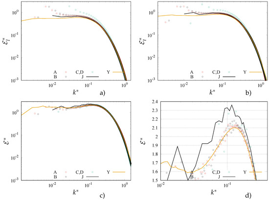
Figure 1.
One- and three-dimensional compensated energy spectra , for flow cases (circles), compared with spectra reported by Jiménez et al. [17] (black line), and by Donzis et al. [2] (yellow line). (a) One-dimensional longitudinal spectra; (b) one-dimensional transverse spectra; (c) compensated three-dimensional spectra in logarithmic scale; (d) compensated three-dimensional spectra in semilogarithmic scale.
The differences in the spectra at low and intermediate wavenumbers can indeed be observed in cases C and D, which have a large and sufficient resolution to simulate the evolution of the thermal field at high Schmidt numbers. The compensated spectra in Figure 1 highlight these differences and emphasize the amplitude of the spectral “bottleneck” phenomenon, namely the energy pile-up at the start of the dissipative range. It is worth noting that the one-dimensional spectra of Donzis et al. [2] in Figure 1 were derived from the three-dimensional spectra using the relationships reported by Pope [18] (p.216). Comparing the three-dimensional spectra in Figure 1c, it can be observed that they exhibit a better agreement. Both types of simulations, using the stochastic forcing scheme and the present simulations in physical space, produce a spectral bottleneck with a significant amplitude. These findings support the conclusions of Bogucki et al. [19], Dobler et al. [20], who argued that a strong bottleneck is only observed in numerical simulations, in which three-dimensional spectra can be directly evaluated. In contrast, experimental spectra are generally derived from frequency spectra using the Taylor hypothesis, which explains why a clear spectral bottleneck is not observed.
In their work, Su et al. [21] conducted a comprehensive analysis of three-dimensional spectra obtained from direct numerical simulations. In Figure 2 of their study, they presented compensated spectra, highlighting their collapse around a peak that varied between a value of 2.2 at and 2.0 at , located at . The present data for cases A and B, shown in Figure 1d, exhibit a good agreement with the spectra reported by Donzis et al. [2] at , using the same scaling as in Su et al. [21]. On the other hand, the spectra of cases C and D align well with those presented by Jiménez et al. [17] at . This agreement further supports the consistency between the present simulations and the findings reported in the literature.
The global data presented in Table 2 provide insights into the variations of quantities related to the passive scalar with the Schmidt number. It is noteworthy that for all cases, the maximum value of indicates that even at the highest , Equation (2) is fully resolved. Furthermore, increases with the Peclet number (). The data in Table 2 suggest an approximate relationship , implying that the scalar dissipation rate remains nearly constant. It is important to note that this relationship only holds for the simulations with a constant , leading to the exclusion of flow case D, where varied. This observation highlights the influence of the forcing method on the computed results.
To validate the passive scalar results at , a comparison was made with the pseudospectral simulation by Donzis et al. [2], denoted as case E in the present study. Although the forcing method in Donzis et al. [2] did not maintain a constant , their higher resolution diminished the impact of the forcing method. The compensated three-dimensional spectra of the passive scalar and energy in Figure 2a demonstrate a good agreement between the present simulations and the results of Donzis et al. [2]. In our simulations, the relatively short inertial range was primarily due to reaching a lower Reynolds number () with a resolution of , which was smaller than the resolution used by Donzis et al. [2] to achieve . Both simulations, however, indicate a larger amplitude of the passive scalar spectral bottleneck compared to that of the velocity field. This difference can be attributed to the different geometry of vortical structures and scalar gradient structures, as commented later. Figure 2b illustrates that similar to the velocity field, the amplitude of the spectral bottleneck in the three-dimensional spectrum of the passive scalar is larger than that in the one-dimensional spectrum. This observation suggests that our low-wavenumber forcing method leads to a less pronounced increase in the amplitude of , particularly in the three-dimensional spectrum.
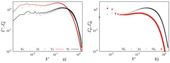
Figure 2.
(a) Three-dimensional compensated energy spectra (, red circles) and compensated passive scalar spectra (, black circles) at , in Kolmogorov units, compared with those of Donzis et al. [2] (lines); (b) three-dimensional passive scalar spectra (black circles) and one-dimensional spectra () along direction (open circles), and along direction (solid circles).
3.2. Effects of Schmidt Number on Spectra
Efforts have been made in the past to provide a theoretical justification for the presence of a range in three-dimensional spectra at high Schmidt numbers, following the inertial range and preceding the exponential decay range. The work of Batchelor [22] played a significant role in this regard, arguing that scalar fluctuations existed only in regions where the spatial variations of the velocity field were linear. These fluctuations can be expressed as the product of the principal strain rates and the position in that eigenframe. Furthermore, Batchelor [22] assumed that the strain rates were locally uniform in space for wavenumbers much larger than the Kolmogorov wavenumber () and persistent in time, neglecting temporal fluctuations. In that scenario, the fluctuating scalar gradients align preferentially with the eigenvector corresponding to the most compressive principal strain rate, denoted as . This alignment leads to the emergence of a range in the scalar spectra. The work of Donzis et al. [2] revisited and expanded upon the arguments put forth by Batchelor [22] to understand the behavior of passive scalar fluctuations in turbulent flows. They considered the effects of strain rates, spatial uniformity, and temporal persistence on scalar gradients, particularly in the context of high Schmidt numbers.
The theoretical considerations of Batchelor [22] led to an expression for the three-dimensional scalar spectrum, which takes into account the effects of strain rates and spatial variations in the velocity field,
where is the scalar dissipation rate, is the Kolmogorov timescale, and is the Batchelor scale. The constant is approximately equal to two and is determined by the average value of the compressive principal strain rate, denoted as . Surprisingly, in the present simulations, was found to be in the range of . This suggests that the compressive strain plays a crucial role in determining the presence of the range in the scalar spectra preceding the bottleneck. Furthermore, it can be speculated that the different actions of the three principal strain rates () on the velocity and scalar fields may be responsible for the formation of scalar gradient structures with a different shape compared to vortical structures. This observation is supported by the absence of a range in the energy spectrum shown in Figure 1, indicating that the dynamics of velocity fluctuations are not controlled by the same mechanisms as scalar fluctuations.
The results of the present simulations are divided into two groups based on the resolution used: one group with a resolution of for low and intermediate Schmidt numbers, and another group with a resolution of for high Schmidt numbers. The compensated spectra for these groups are shown in Figure 3, with Figure 3a,b representing the simulations, and Figure 3c,d representing the simulations. The figures demonstrate a significant collapse of the spectra in the dissipation range, starting at . At low wavenumbers, the compensated spectra exhibit a plateau value () over a certain range of wavenumbers, which is not easily discernible due to the scalar forcing for . The spectra from the simulations (top panels) show a larger number of data points at low and match well with the constant value . The dependence of on the Schmidt number can be observed in Figure 3b,d, which have scales similar to those in Figure 2 of Su et al. [21]. The transition from the inertial range to the exponential decay range is characterized by a reduction in the slope of , which is required to have a maximum value which is independent of .
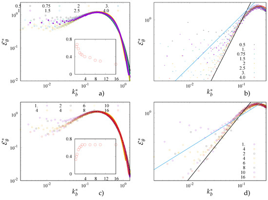
Figure 3.
Three-dimensional compensated passive scalar spectra () for simulations with (a,b) and with (c,d), reported as a function of . Values of the Schmidt number are indicated in the legend; in the inset of (a), versus is reported; in the inset of (c), n versus is reported. In (b,d), the blue line refers to , and the black line to . The solid purple dots in (a,b) refer to case E1 reported in Table 2
The range of where the transition from the inertial range to the exponential decay range occurs increases with the Schmidt number. Within this range, the slope of exhibits a variation from to . These two limits correspond to power laws () with and , respectively. By analyzing the data plotted in Figure 3, the variations of and n with have been evaluated and are shown in the insets of Figure 3a,c. It is worth noting that the value of predicted by Batchelor [22] can be observed for . Additionally, as discussed earlier, the range of where increases with an increasing .
3.3. Dissipation Spectra and PDFs in the Principal Strain Axes
Figure 4a provides a clear visualization of the amplitude of the spectral bottleneck by plotting the energy and passive scalar dissipation spectra. The collapse of the spectra in Kolmogorov units is shown for both the A and C cases, indicating the range of wavenumbers in which collapse occurs. In physical space, the shape of the spectra at high wavenumbers is determined by the vorticity field and by the scalar gradients. Figure 4a reveals that the largest content of energy and scalar dissipation resides at wavenumbers corresponding to the maximum of the spectral bottleneck. This observation suggests that the size of the vorticity structures is greater than that of the passive scalar gradients. Furthermore, it is expected that the probability distribution functions (PDFs) of the vorticity components () and the passive scalar gradients () in forced isotropic turbulence are approximately independent of their direction. However, these PDFs are not specifically shown in the figure.
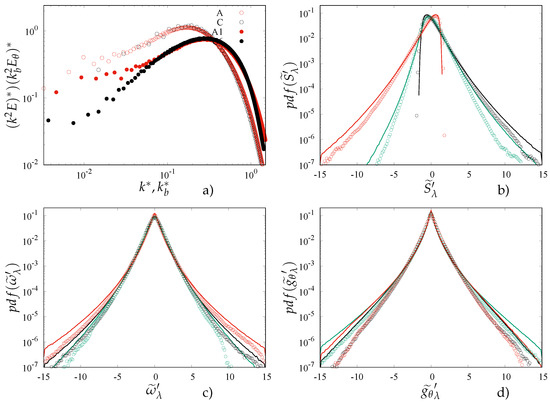
Figure 4.
(a) Three-dimensional energy dissipation spectra (open circles), and passive scalar dissipation spectra (solid circles) for flow cases A (red) and C (black); (b) PDF of the principal strain rates (), (c) PDF of the vorticity components in the principal strain axes (), and (c) PDF of the scalar gradient components in the principal strain axes (), for an extensional stress (, black), intermediate stress (, green), and compressive stress (, red), Lines are used for case A, and symbols for case C.
To understand the flow physics in greater detail, the evolution of vorticity components can be analyzed by projecting them along the principal axes of the strain rate tensor. The strain rate tensor eigenvalues, denoted as , provide valuable information about the flow characteristics. The incompressibility condition requires the sum of these eigenvalues to be zero. Among the three eigenvalues, is the largest and positive, while is the smallest and negative. The sign of the intermediate eigenvalue, , determines the sign of the determinant . This determinant, in turn, determines the nature of the vortex structures near a specific point in space. If , the structures are rodlike, whereas if , they are sheetlike. From various databases of turbulent flows, including forced and decaying flows, as well as wall-bounded and free-shear flows, it has been observed that sheetlike regions dominate. These sheetlike structures are more unstable and play a significant role in the energy cascade process [23].
Previous studies have also explored the flow topology associated with concentrations of scalar gradients. One notable finding by Kerr [24] was that while vorticity is concentrated in tube-like structures, the scalar gradient and the largest principal rate of strain align perpendicular to these tubes. Kerr [24] also observed that the highest values of the scalar gradient occurred in sheets that wrapped around the vortical tubes. However, the simulations in Kerr’s study were conducted at lower Reynolds numbers than in the present study. In addition to studying the flow topology, the present study also focused on examining the enstrophy and scalar gradient variance budget equations, specifically their alignment with the principal axes of the strain rate tensor. These investigations aimed to provide further insights into the flow dynamics and the role of different terms in the budget equations.
At each point in the computational domain, the strain rate tensor was evaluated, and its eigenvalues and eigenvectors were determined. These eigenvalues and eigenvectors were used to calculate the respective components of the vorticity vector () and of the scalar gradient vector (). To analyze the statistics of these quantities, the normalized PDFs of the generic quantity q were considered, with , where denotes the average value over the entire computational domain. In Figure 4b, the PDFs of the three components are shown. The compressive strain component () is depicted in red and exhibits a negative skewness, indicating a concentration of intense negative values. On the other hand, the extensional strain component () is shown in black and exhibits a positive skewness, indicating a concentration of intense positive values. The magnitude of events in is generally stronger than that in , and this magnitude tends to increase with the Reynolds number. It is worth noting that the intermediate component can take both positive and negative values, and consistent with previous findings, the determinant is negative for all flow cases, indicating a prevalence of sheetlike structures over rodlike structures.
Table 3 provides the values of the skewness () and flatness () coefficients for the strain fluctuations, as obtained from the PDFs shown in Figure 4b. These coefficients quantify the differences in the distributions of the strain components. The larger value of compared to indicates a higher amplitude of events for the compressive strain component () compared to the extensional strain component (). This observation supports the formation of high-amplitude events for . Additionally, the positive skewness coefficient indicates a prevalence of positive events for the intermediate strain component (), contributing to the overall negative value of . The flatness coefficient suggests that the amplitude of events for is smaller compared to the compressed and extensional strain components. In Figure 4c, the PDFs of the vorticity components aligned with the are shown. The symmetric distribution of these components is evident, as indicated by the low values of the skewness coefficients () presented in Table 4. The negative values of the skewness coefficients, however, highlight a negative skewness of the vorticity components, which is not easily discernible in Figure 4c. It is noteworthy that the symmetry of the events decreases with an increasing Reynolds number, as observed in the table and the figure, as well as in the other flow cases (B and E), which are not shown here.
Table 3.
Skewness () and flatness () coefficients for the principal strain rates ().
Table 4.
Skewness () and flatness () coefficients for the vorticity components in the principal strain axes ().
Table 5 provides the skewness and flatness coefficients for the normalized scalar gradient components (), and these coefficients show relatively small differences compared to those of the vorticity components () presented in Table 4. However, the flatness coefficients for the scalar gradients are generally larger than those for the vorticity components. These findings, along with the spectra shown in Figure 4, suggest that the scalar gradient structures are thinner and more intense compared to the vorticity structures. To gain further insight into this behavior, the enstrophy and scalar gradient variance budgets of the components along the principal axes are analyzed in the subsequent sections.
Table 5.
Skewness () and flatness () coefficients for the scalar gradient components in the principal strain axes ().
3.4. Enstrophy Budgets
The budget equation for the time-averaged enstrophy, , expressed in terms of the quantities in the principal strain rate axes is given by
In this equation, the rate of entropy dissipation was evaluated by projecting on the principal axes of the strain tensor the three components of the Laplacian of the vorticity vector, and the quantities obtained were then multiplied by and summed over . It is noteworthy that an accurate evaluation of the enstrophy dissipation rate requires a proper resolution of the compensated spectra, which we preliminarily checked.
The and the events are the contributors to , which motivates an in-depth analysis of their correlation. The values of each component of are reported in Table 6, which shows that the intermediate stress contribution is comparable to that of the extensional one. On the other hand, the component aligned with the compressive strain is the smallest, and its intrinsic negative sign reduces the overall enstrophy production. To understand whether and how events containing and are correlated, the joint PDF between and are shown in Figure 4. Small differences between the distributions at high and low Reynolds number have been found, although only the flow case is shown. In the analysis of Figure 5, it is important to recall that the skewness of the vorticity components is small, hence the joint PDF are nearly symmetric with respect to the horizontal axis, and the correlation coefficients between and are thus small. The extensional strain (Figure 5a) and compressive strain (Figure 5c) have rather different distributions. The asymmetric distribution of and discussed in Figure 4 contributes to the different behavior observed in quadrants I and compared to quadrants and (see Figure 5a,c). To gain more insight into the difference between the compressed and extensional stress, the contributions of each quadrant to the correlation coefficients are isolated in Table 7. The first quadrant for the extensional stress contributes almost twice as much as the compressed stress, and the same occurs for the fourth quadrant. The values in the table quantify the higher contributions of quadrant I for the compressed stress compared to that of quadrant for the extensional stress. Similarly, there is a higher contribution from quadrant I for the extensional stress compared to quadrant for the compressive stress. This indicates that events with high magnitudes of the stress are associated with the generation of strong vorticity components aligned with them.
Table 6.
Enstrophy production (), and scalar gradient variance production ().
Table 7.
Contributions to from each quadrant, evaluated from the joint PDF in Figure 5.
The joint PDF between the intermediate strain and the associated vorticity component in Figure 5b exhibits a different distribution compared to the previous cases. However, the contributions from each quadrant are similar to those of the extensional stress, as shown in Table 7. Despite the global lack of correlation between the strain and vorticity components, their interaction contributes to the positive enstrophy production, as seen in Table 6. To further analyze the enstrophy production, the joint PDF between and is evaluated. The PDF of is positively skewed, so the range of was taken from to 7, while the range of was to 15. The normalized joint PDF reveals that the four quadrants are no longer balanced, as shown in Table 8.
Table 8.
Contributions to from each quadrant, evaluated from the joint PDF between and .
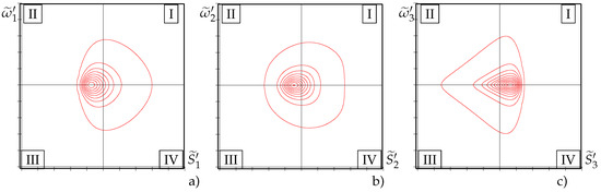
Figure 5.
Joint PDF between normalized principal strain fluctuations (, horizontal axis) and corresponding vorticity fluctuations (, vertical axis), for flow case ; (a) extensional strain, (b) intermediate strain, and (c) compressive strain. Contours are shown with spacing Roman numbers denote the four quadrants.
The high positive values of and indicate a large contribution from quadrant I (see Table 8). The contribution of quadrant to is smaller compared to , resulting in . On the other hand, the negative value of is due to the negative contributions from quadrants and , which are larger than the positive contributions from the other quadrants. However, none of these contributions is comparable in magnitude to the positive ones for and . This explains why is smaller than .
3.5. Budget of Scalar Gradient Variance
The budget equation for the scalar gradient variance , is expressed as
where the rate of scalar gradient dissipation is evaluated by projecting the three components of the Laplacian of the scalar gradient onto the principal axes of the strain rate tensor, multiplying by , and then summing over . As for the enstrophy dissipation, we verified that the compensated spectra decayed at the highest k, hence supporting that the scalar gradient dissipation was properly resolved.
Differences between the terms in Equations (7) and (8) were discussed by Tsinober and Galanti [25], who emphasized the different signs of the production terms. The values presented in Table 6 indeed demonstrate that for the scalar gradient variance, the positive contribution from the compressive strain dominates over the other two components, and the contribution from the intermediate strain is the smallest. Notably, this dominance of the compressive strain contribution is independent of the Peclet number, as evident from the values reported in Table 6 for the high Reynolds number case () and for the low Reynolds number case ().
3.5.1. Rate of Production of Scalar Gradient Variance
The joint PDF between and was evaluated, demonstrating a good independence from the Peclet number. As a result, Figure 6 displays the distributions for flow case only. Choosing a flow with makes the analysis of the differences between the interactions of strain with vorticity and scalar gradients more instructive, as does not affect the rate of scalar gradient dissipation, see Equation (8). In Figure 5, the three joint PDF differ significantly from each other. However, in Figure 6, the three joint PDF distributions are more similar, when considering the asymmetry of the PDFs of and . The similarity between the joint PDFs shown in panels (c) of Figure 5 and Figure 6 is a preliminary indication of the importance of the compressive strain in the scalar gradient dynamics.
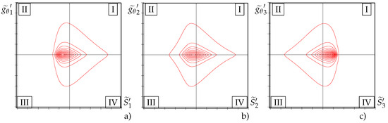
Figure 6.
Joint PDF between normalized principal strain fluctuations (, horizontal axis) and corresponding scalar gradient fluctuations (, vertical axis), for flow case (, contours with interval ): (a) extensional strain, (b) intermediate strain, and (c) compressive strain. Roman numbers denote the four quadrants.
The symmetry of the joint PDFs with respect to the horizontal axis is also observed for the passive scalar gradient components. To quantify their magnitude, the contributions of each quadrant to the correlation coefficient are reported in Table 9. A quick examination reveals that in this case as well, the quantities are uncorrelated. The negative contributions from quadrant for the component are the largest, resulting in the sum of the three values being larger than that of . Table 9 indicates that the four contributions do not differ significantly for . Additionally, Figure 6b demonstrates that in this case, the distribution contours in the four quadrants are dissimilar, unlike in Figure 5b. The equilibration is attributed to the positively skewed distribution of and to the occurrence of strong events.
Table 9.
Flow case A2: contributions to from each quadrant, as from the joint PDF reported in Figure 6.
The interaction between the and events contributes significantly to the positive value of in the scalar gradient production (see Table 6). To further understand the large differences among the three contributions to the scalar gradient production, the joint probability density function (PDF) between and was evaluated. The PDF of exhibited a high positive skewness. Similar to , the joint PDF of and was evaluated by varying the interval for between and 7, and the interval for between and 15. From the normalized joint PDF, the quadrant contributions to each component of were evaluated. Table 10 reveals that the distributions in the four quadrants are no longer equilibrated.
Table 10.
Flow case A2: contributions to from each quadrant, evaluated from the joint PDF between and , evaluated for .
The high positive values of can be attributed to the negative contributions from quadrants and (see Table 10), which outweigh the positive contributions from the other two quadrants. As for the contribution, there is an increased equilibration among the quadrants, resulting in a small value of the correlation coefficient. This explains why reported in Table 7 is much smaller in magnitude compared to the other two components.
3.5.2. Rate of Dissipation of Enstrophy and Scalar Gradient Variance
In the study by Orlandi et al. [4], a “minimal flow unit” was employed to investigate the potential finite-time singularity of the Euler equation by tracking the evolution of relevant statistics. In the viscous case, the evolution of these statistics depended on the Reynolds number. The initial conditions for the “minimal flow unit” consisted of two orthogonal Lamb dipoles positioned at a certain distance from each other. The self-induction effect caused the dipoles to approach and eventually collide. During that time evolution, a range of small vortical structures formed, which were distinct from those observed in the inviscid evolution. The spectra of velocity and passive scalar at a specific time during the viscous collision were found to agree with those of the forced isotropic turbulence. This transition from a vorticity-dominated to a turbulent stage allowed for a connection between the evolution of spectra and the visualization of flow structures in physical space.
In the present paper, before presenting the visualizations of the quantities involved in Equations (7) and (8), it is important to present the averaged values for different combinations of Schmidt and Reynolds numbers. The production of enstrophy and scalar gradient variance, as shown in Table 7, should be balanced by the rate of dissipation of enstrophy and scalar gradient variance, reported in Table 11. It is important to note that these terms are evaluated from individual fields, so the global balance observed when aggregating a large number of fields may not hold. The values reported in Table 11 highlight that the component aligned with the intermediate strain contributes the most to the rate of enstrophy dissipation, while the component aligned with the compressive strain contributes the least. On the other hand, the rate of scalar gradient variance dissipation is largely attributed to the component aligned with the compressive strain. For the simulations denoted as A and C in Table 1, the ratio varied between 0.2 and 0.25 for , whereas the ratio was approximately 0.025. In contrast, the dissipation of scalar gradient variance shows a dependence on the Schmidt number. For case A, the ratio ranged from 0.17 to 0.27, and ranged from 0.12 to 0.20. In the case of C, the variation was minimal, with and .
Table 11.
Rate of enstrophy dissipation (), and scalar gradient dissipation ().
4. Flow Visualizations
4.1. Vorticity, Strain, and Scalar Gradient
The shape and size of the intense vorticity structures in the flow differ from those where scalar gradients are intensified. This distinction is qualitatively represented by the velocity and scalar spectra. By conducting flow visualizations, it is possible to investigate the association of zones with an intense enstrophy density () and high scalar dissipation density (), and regions of intense strain magnitude (). In forced isotropic turbulence, several regions with intense turbulent activity are observed. However, due to the three-dimensional nature of the flow, the visualizations are not as clear as those presented in Orlandi et al. [4], where a hierarchy of turbulent structures formed in the small region where the Lamb vortices collided. In the present flows, two-dimensional visualizations were performed in a plane defined by the and coordinates, covering the entire computational domain (). These visualizations revealed several spots with a high enstrophy and scalar gradient variance. To obtain a clear view of these turbulent structures, visualizations were performed for the case at a low Reynolds number and , focusing on a limited area (). For the flow case at a high Reynolds number and , the structures were smaller compared to those in the case. Therefore, the visualization area was further reduced to .
The normalized fluctuations of the above properties (, , ) can take both positive and negative values, indicating contributions greater or smaller than their mean values, respectively. These quantities are used to generate normalized PDFs and planar visualizations, as shown in Figure 7. The top row of Figure 7 shows that the three PDFs do not exhibit significant differences, and the probability of obtaining values that are five times greater than their root-mean-square value is relatively small. Furthermore, the positive tail of the PDFs is the same for both the and flows. The insets in Figure 7b,c indicate that there is only a Reynolds number effect on the negative values, which are associated with the shape and size of the large scales. From the PDFs alone, it can be concluded that they do not provide indications of the influence of the Reynolds number and Schmidt number on the shape and intensity of the structures.
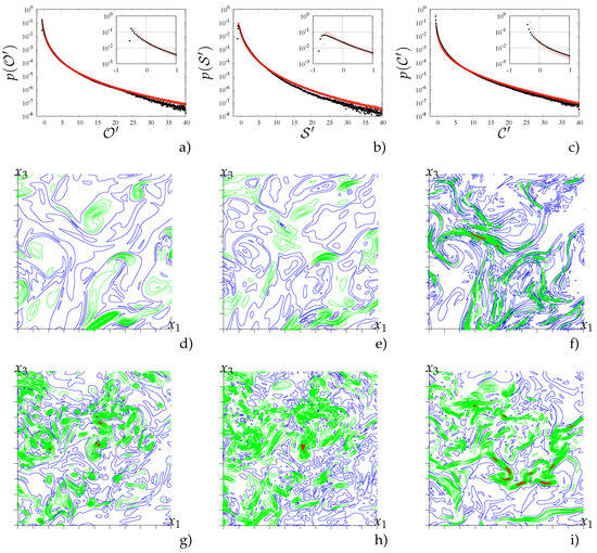
Figure 7.
PDF of enstrophy density (, panel (a)), strain magnitude (, panel (b)), and scalar gradient magnitude (, panel (c)) (flow case in red, flow case in black), and visualization of the same quantities for flow case (panels (d–f), in the range ), and flow case for (panels (g–i), in the range ). Negative contours are shown in blue, with increment , and positive contours are shown in green (values ), and in red contours (values ), with increment .
However, such influences can be appreciated through the visualizations of the enstrophy, strain, and scalar gradient variance contours presented in Figure 7. In that figure, negative values (blue contours) occupy a large part of the flow, whereas positive fluctuations (red and green contours) are concentrated in small regions. At low Reynolds number, the contours of (Figure 7d) and (Figure 7e) are organized into larger patterns compared to those at high (see Figure 7g,h). This difference is even more apparent when considering that the areas which are depicted is four times smaller. The visualizations at low of contours of superimposed to those of highlight the strong probability that regions with a large are located near regions with a strong .
To quantify the correlation between the various quantities, the corresponding joint PDFs were evaluated, and the quadrant contributions to the correlation coefficients are shown in Table 12, where a and b denote any two generic quantities. The correlation coefficient between and is quite large and relatively independent of the Reynolds number. The first quadrant contributes the most, indicating that high and positive values of are associated with points of intense . Points with small negative values of and contribute to to a lesser extent, while the negative contribution to from and of opposite sign is negligible. The influence of the compressive strain on the passive scalar leads to elongated patterns of at low and (see Figure 7f). This figure, together with Figure 7e, indicates that the correlation coefficient between the and events is small, as corroborated by the quadrant contributions in Table 12. Although is reduced, Table 12 emphasizes that the first quadrant contributes the most. Even at high and (see Figure 7i), the patterns of are still rather elongated, with intense positive (red-colored) events poorly correlated with strong positive events. Despite this occurrence, the contribution is greater in the flow case than in the flow case. From the table, it can be concluded that the correlation coefficient reduces with an increase in .
Table 12.
Contributions to correlation coefficients from each quadrant of the joint PDF, related to the visualizations reported in Figure 7.
4.2. Enstrophy and Scalar Gradient Variance Budgets Terms
To better understand the differences between the patterns of and , it is useful to analyze the distributions of the respective terms in their budget equations, Equations (7) and (8), using the PDFs and planar visualizations of the production and dissipation terms. Figure 8 shows the visualizations corresponding to the and cases. The PDFs of the enstrophy dissipation density (, Figure 8b) and of the scalar gradient dissipation density (, Figure 8d) are similar and independent of the flow case. The insets emphasize that this similarity holds even for the low-amplitude events. The PDF of the enstrophy production density (, Figure 8a) exhibits a good independence with respect to the Reynolds number. Since the positive events are stronger than the negative ones, their skewness coefficients are approximately equal to seven. On the other hand, regarding the scalar gradient production density (, Figure 8c) the positive events are much stronger than the negative ones, indicating a prevalence of the compressive stress over the extensional stress in the formation of strong scalar gradients. The inset in Figure 8c shows a dependence on the Schmidt number for the weak events, but this does not affect the high skewness coefficient, which is equal to 10.5.
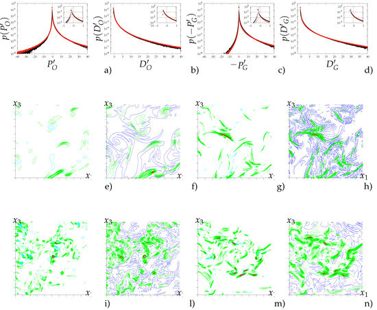
Figure 8.
PDF of enstrophy production density (, panel (a)), enstrophy dissipation density (, panel (b)), scalar gradient production density (, panel (c)), (flow case in red, flow case in black) and scalar gradient dissipation density (, panel (d)), and visualization of the same quantities for flow case (panels (e–h), in the range ) and flow case for (panels (i–l), in the range ). Negative contours are shown in blue, with increment , and positive contours are shown in green (values ) and in red contours (values ), with increment .
At low , the positive events in Figure 8 are observed to occur within large-size regions, and there is a strong correspondence between negative values of enstrophy production in Figure 8e and zones depleted with enstrophy dissipation in Figure 8f. However, there is a good correlation between the positive events, as evidenced by the dominance of the first quadrant contribution () over the others. Thin and elongated regions with large positive scalar gradient production (Figure 8g) and scalar gradient dissipation (Figure 8h) are also observed, which reduce the correlation coefficient (), consistent with the visualizations in Figure 7. At high , a similar behavior is observed in the bottom figures. The Reynolds number independence is demonstrated by for the correlation coefficient between the terms of Equation (7). There is a slight increase in the correlation between scalar gradient production and scalar gradient dissipation with the Schmidt number, as shown by for the case.
4.3. Identification of Enstrophy- and Vorticity-Containing Structures
Figure 9a,b present isosurfaces of the enstrophy dissipation density (), of the enstrophy production density (), and of the Q criterion [26], all normalized by the mean enstrophy. These visualizations aim to explore the potential correspondence between the terms in Equation (7) and rod- or ribbonlike structures. Visualizations for flow case of (low , ) are shown in Figure 9. The Q criterion, introduced by Jeong and Hussain [26], is a popular method for distinguishing between rodlike and ribbonlike structures in turbulent flows. It is defined as , evaluated with the components projected on the principal axes. Structures with are considered rodlike, while those with are classified as ribbonlike. Three-dimensional visualizations of enstrophy dissipation density (), enstrophy production density (), and Q, all normalized by the mean enstrophy, can help investigate the correspondence between these terms in Equation (7) and rod- or ribbonlike structures. Figure 9a,b show such visualizations for the case at low Reynolds number and . In these figures, the red surfaces, depicted as circular shapes, represent rodlike structures with , while the blue surfaces correspond to ribbonlike structures with . It is important to note that these visualizations were performed in a small region, and thus the observed volume may not be representative of the entire flow. However, it appears that regions dominated by vorticity occupy a larger volume compared to those dominated by strain. By measuring the volume occupied by the (blue) and (red) regions in the entire computational box, it was found that the former accounted for of the volume, while the latter occupied . This observation can be explained by considering that under the constraint , the amplitude of the patches is smaller than that of the patches. In Figure 9a, the formation of yellow layers, indicating a positive , can be observed primarily close to or within the rodlike structures. Figure 9b shows that the negative green regions representing are small, rare, and predominantly occurring in regions with a weak Q.
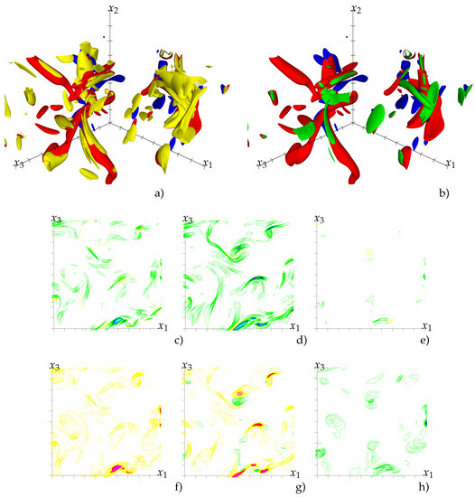
Figure 9.
Isosurfaces of (red positive, blue negative) superposed on (a) isosurfaces of (yellow positive, green negative); (b) isosurfaces of (yellow positive, green negative); (c–e) contours of contributions to enstrophy dissipation in the principal strain axes (); (f–h) contours of contributions to enstrophy production in the principal strain axes. (); (c,f) extensional, (d,g) intermediate, (e,h) compressed. Green and blue are used for negative values and yellow, red and magenta are used for positive values, with contour increment .
The distribution of the enstrophy production and dissipation densities can be better understood through contour plots in planar sections. From these plots and Figure 9b, it is evident that the dissipation density is mainly concentrated within the rodlike structures, while only a few spots are located in regions of weak Q. Additionally, locally, the enstrophy dissipation density may take small positive values, which are mostly located outside the rodlike structures. By examining the contour plots in the plane at the center of the computational box, one can investigate the contributions of each component to the enstrophy balance. In Figure 9c–e, the green regions representing the negative rate of enstrophy dissipation accumulate in elongated patches. The largest contribution comes from the component in Figure 9d, while the contribution from the component in Figure 9e is marginal. In Figure 9h, the component of enstrophy production along is negative and smaller than the other two components. Also for enstrophy production, the contribution (Figure 9g) reaches high values. It is worth noting that the component, as observed in inviscid simulations by Orlandi et al. [4] of interacting Lamb dipoles, leads to an extreme growth of enstrophy, which is a key factor in the eventual formation of a singularity.
4.4. Structures Associated with Scalar Gradients
The visualizations of the terms in the scalar gradient balance equation (Equation (8)) provide insights into the differences with terms in the enstrophy balance equations. While previous studies [5] discussed these differences at low and , they did not emphasize the relative contributions of each component along the principal axes of the strain field. To obtain clearer visualizations, the results of the scalar gradient balance terms are shown for instead of . Figure 9a,b and Figure 10a,b highlight the accumulation of the scalar gradient production term in sheets that are separate from regions with . At , these sheets of high production become thinner and wider compared to those shown in Figure 10a. Figure 10b illustrates that the scalar gradient dissipation is concentrated in thin layers located where Q is weak. Furthermore, the contributions of the three contributions to the scalar gradient production and dissipation in the principal strain axes are found to be significantly different from the corresponding contributions to the enstrophy production and dissipation. Specifically, Figure 10d,g demonstrate that the contribution of the components is relatively small compared to the other components. The strongest contributions in the scalar gradient balance equation come from the compressive strain, as quantified in Table 6 and Table 11. Figure 10e further illustrates that this component has greater positive contributions to the scalar gradient dissipation compared to the other components. The compressive strain is responsible for the strongest contribution to production, as depicted in Figure 10h and Table 6. It is important to note that in Equation (8), the production term has a negative sign, so the negative green lines in Figure 10h indicate a positive contribution. On the other hand, the extensional strain component gives a negative contribution to the formation of the strong thin layers of the scalar gradient. Figure 10f demonstrates that this component is located in the same regions as those for the enstrophy dissipation in Figure 10c. Indeed, the visualizations provide valuable insights and corroborate the different effects of the strain field on the vorticity and passive scalar gradient components. They allow for a deeper understanding of the spatial distribution and interactions of these quantities, highlighting the regions where they are concentrated and the relationships between them. By examining the visualizations, one can gain a more comprehensive knowledge of how the strain field influences the dynamics of vorticity and passive scalar gradients in the flow.
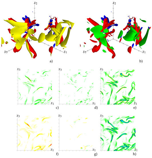
Figure 10.
Isosurfaces of (red positive, blue negative) superposed on (a) isosurfaces of (yellow positive, green negative); (b) isosurfaces of (yellow positive, green negative); (c–e) contours of contributions to scalar gradient dissipation in principal strain axes (); (f–h) contours of contributions to scalar gradient production in principal strain axes (); (c,f) extensional, (d,g) intermediate, (e,h) compressed. Green blue and cyan are used for negative values and yellow red and magenta are used for positive values, with contour increment .
5. Conclusions
The study of passive scalar advection by turbulent velocity fields has been a subject of extensive research. Previous work, such as the review by Warhaft [27], examined this topic from experimental and theoretical perspectives. Donzis et al. [2] conducted well-resolved direct numerical simulations (DNS) to investigate the influence of Schmidt number variations on scalar statistics, which was also previously reviewed by Antonia and Orlandi [28]. The focus of the present study was to quantify the dependence of the slope of the transitional range in the nondimensional passive scalar spectra on the Schmidt number. This transitional range connects the inertial range (spectral slope ) of the compensated scalar spectra, at low wavenumbers, to the slope associated with the spectral bottleneck, which occurs at a fixed nondimensional wavenumber as described by Batchelor [22]. In the compensated scalar spectrum at low wavenumbers, there was a constant value which decreased with an increasing Schmidt number. However, the evaluation of the spectrum at extremely low and high values required a large number of grid points in the simulations to minimize the effect of forcing on the low wavenumber spectra. On the other hand, the dependence of the spectral slope n of the transitional range on the Schmidt number was measured, and it was found that for , the slope remained fixed at [2]. This indicates that the scaling behavior in the transitional range is independent of the Schmidt number for values above a certain threshold.
A further investigation using refined DNS techniques based on codes optimized for GPU clusters, such as CUDA Fortran and OpenACC directives, along with the use of CUFFT libraries for efficient FFT execution, were used to provide valuable insights into the points mentioned. The comparison between the three-dimensional energy dissipation and passive scalar dissipation spectra highlighted the presence of spectral bottlenecks in both quantities. The compensated nondimensional passive scalar spectra exhibited a bottleneck with a maximum value and a wavenumber location that was independent of the Schmidt number. Notably, this nondimensional wavenumber was higher than that associated with the vortical structures. To further investigate the underlying physics, the strain rate tensor was evaluated at each computational point. The vorticity and scalar gradient vectors were projected along the principal axes of , and the joint probability density function (PDF) among them and provided insights into the distinct roles played by the components of in the generation of vorticity and passive scalar gradient structures. This analysis allowed for a more comprehensive understanding of the dynamics and interactions between velocity and scalar fields in turbulent flows.
Investigating the influence of different vortical structures on passive scalar dynamics is an important research direction that can provide valuable insights. Adding solid body rotation to the flow presents an interesting case to explore using the same code and numerical framework as in the current study. In the presence of high rotation rates, the velocity spectra tend to exhibit a inertial range, indicating the presence of more elongated vortical structures aligned with the rotation axis. Preliminary simulations suggest that for the passive scalar, the spectra maintain a range over a wide range of wavenumbers. However, a more detailed analysis similar to the one performed in this paper is necessary to understand this behavior and its implications. Understanding why solid body rotation does not significantly affect the passive scalar spectra can have important implications, particularly in the field of combustion. The complex physics of passive scalar dynamics in rotating chambers can potentially lead to the design of more efficient engines. Therefore, further investigations into the interaction between rotation and passive scalar transport can contribute to advancements in combustion science and technology.
Author Contributions
Conceptualization, P.O.; methodology, P.O.; software, P.O.; formal analysis, S.P.; writing—original draft preparation, P.O.; writing—review and editing, S.P. All authors have read and agreed to the published version of the manuscript.
Funding
This research received no specific grant from any funding agency, commercial or not-for-profit sectors.
Data Availability Statement
The data that support the findings of this study are openly available at the web page http://newton.dma.uniroma1.it/database/.
Acknowledgments
The authors acknowledge that some of the results reported in this paper have been achieved using the PRACE Research Infrastructure resource Marconi-100 based at CINECA, Casalecchio di Reno, Italy.
Conflicts of Interest
The authors declare no conflict of interest.
References
- Ishihara, T.; Gotoh, T.; Kaneda, Y. Study of high-Reynolds-number isotropic turbulence by Direct Numerical Simulation. Annu. Rev. Fluid Mech. 2008, 41, 165–180. [Google Scholar] [CrossRef]
- Donzis, D.; Sreenivasan, K.; Yeung, P. The Batchelor Spectrum for mixing of passive scalars in isotropic turbulence. Flow Turbul. Combust 2010, 85, 549–566. [Google Scholar] [CrossRef]
- Orlandi, P.; Antonia, R.A. Dependence of a passive scalar in decaying isotropic turbulence on the Reynolds and Schmidt numbers using the EDQNM mode. J. Turbul. 2004, 5, 009. [Google Scholar] [CrossRef]
- Orlandi, P.; Pirozzoli, S.; Bernardini, M.; Carnevale, G. A minimal flow unit for the study of turbulence with passive scalars. J. Turbul. 2014, 15, 731–751. [Google Scholar] [CrossRef]
- Tsinober, A. An Informal Introduction to Turbulence; Kluwer Academic Publisher: Norwell, MA, USA, 2000. [Google Scholar]
- Lohse, D. Temperature spectra in shear flow and thermal convection. Phys. Lett. A 1994, 196, 70–75. [Google Scholar] [CrossRef]
- Tennekes, H.; Lumley, J.L. A First Course in Turbulence; MIT Press: Cambridge, MA, USA, 1972. [Google Scholar]
- Sreenivasan, K. On local isotropy of passive scalars in turbulent shear flows. Proc. R. Soc. Lond. A 1991, 434, 165–182. [Google Scholar]
- Bolgiano, R. Turbulent spectra in a stably stratified atmosphere. J. Geophys. Res. 1959, 64, 2226–2229. [Google Scholar] [CrossRef]
- Obukhov, A. On the influence of Archimedean forces on the structure of the temperature field in a turbulent flow. Dokl. Akad. Nauk. SSR 1959, 125, 1246–1248. [Google Scholar]
- Camussi, R.; Verzicco, R. Temporal statistics in high Rayleigh number convective turbulence. Eur. J. Mech. B/Fluids 2004, 23, 427–442. [Google Scholar] [CrossRef]
- Lohse, D.; Xia, K. Small-Scale Properties of Turbulent Rayleigh-Bénard convection. Annu. Rev. Fluid Mech. 2010, 42, 335–364. [Google Scholar] [CrossRef]
- Orlandi, P.; Pirozzoli, S. Turbulent spectra in natural and forced convection. Int. J. Heat Mass Transf. 2023, 208, 124032. [Google Scholar] [CrossRef]
- Rogallo, R. Numerical experiments in homogeneous turbulence. NASA Tech. Mem. 1981, 81315. [Google Scholar]
- Eswaran, V.; Pope, S. An examination of forcing in direct numerical simulations of turbulence. Comput. Fluids 1988, 16, 257–278. [Google Scholar] [CrossRef]
- Orlandi, P. Fluid Flow Phenomena—A Numerical Toolkit; Kluwer Academic Publisher: Norwell, MA, USA, 2000. [Google Scholar]
- Jiménez, J.; Wray, A.A.; Saffman, P.G.; Rogallo, R.S. The structure of intense vorticity in isotropic turbulence. J. Fluid Mech. 1993, 255, 65–90. [Google Scholar] [CrossRef]
- Pope, S.B. Turbulent Flows; Cambridge University Press: Cambridge, UK, 2000. [Google Scholar]
- Bogucki, D.; Domaradzki, J.; Yeung, P. Direct numerical simulations of passive scalars with Pr>1 advected by turbulent flow. J. Fluid Mech. 1997, 343, 111–130. [Google Scholar] [CrossRef]
- Dobler, W.; Haugen, N.E.L.; Yousef, T.A.; Brandenburg, A. Bottleneck effect in three-dimensional turbulence simulations. Phys. Rev. E 2003, 68, 026304. [Google Scholar] [CrossRef]
- Su, H.; Yang, Y.; Pope, S. Simple model for the bottleneck effect in isotropic turbulence based on Kolmogorov’s hypotheses. Phys. Rev. Fluids 2023, 8, 014603. [Google Scholar] [CrossRef]
- Batchelor, G. Small-scale variation of convected quantities like temperature in turbulent fluid. General discussion and the case of small conductivity. J. Fluid Mech. 1959, 5, 113–133. [Google Scholar] [CrossRef]
- Horiuti, K.; Fujisawa, T. The multi-mode stretched spiral vortex in homogeneous isotropic turbulence. J. Fluid Mech. 2008, 595, 341–366. [Google Scholar] [CrossRef]
- Kerr, R.M. Higher-order derivative correlations and the alignment of small-scale structures in isotropic numerical turbulence. J. Fluid Mech. 1987, 153, 31–58. [Google Scholar] [CrossRef]
- Tsinober, A.; Galanti, B. Exploratory numerical experiments on the differences between genuine and “passive” turbulence. Phys. Fluids 2003, 15, 3514–3531. [Google Scholar] [CrossRef]
- Jeong, J.; Hussain, F. On the identification of a vortex. J. Fluid Mech. 1995, 285, 69–94. [Google Scholar] [CrossRef]
- Warhaft, Z. Passive scalars in turbulent flows. Annu. Rev. Fluid Mech. 2000, 32, 203–240. [Google Scholar] [CrossRef]
- Antonia, R.; Orlandi, P. Effect of Schmidt number on small-scale passive scalar turbulence. Appl. Mech. Rev. 2003, 56, 615–632. [Google Scholar] [CrossRef]
Disclaimer/Publisher’s Note: The statements, opinions and data contained in all publications are solely those of the individual author(s) and contributor(s) and not of MDPI and/or the editor(s). MDPI and/or the editor(s) disclaim responsibility for any injury to people or property resulting from any ideas, methods, instructions or products referred to in the content. |
© 2023 by the authors. Licensee MDPI, Basel, Switzerland. This article is an open access article distributed under the terms and conditions of the Creative Commons Attribution (CC BY) license (https://creativecommons.org/licenses/by/4.0/).