Abstract
The geometric complexity and high-pressure gradients that characterize the design of the flow field of gear pumps make it very difficult to obtain an accurate CFD simulation of the component. Usually, assumptions are made both in terms of geometrical features and physics being included in the analysis. The contact between the teeth, which is a key factor for the correct functioning of these pumps, represents a critical challenge in 3D CFD simulations, mainly due to the intrinsic limits of the dynamic meshing techniques that can hardly effectively manage a zero or close to zero gap point forming during gear rotation. The geometric complexity and high-pressure gradients that characterize the gear pump flow field make a CFD analysis quite difficult, and the contact between the gear teeth is usually avoided, thus being an extremely important feature. In this paper, a gear pump composed of inlet and outlet pipes was considered, and the contact between the gear’s teeth was modeled in two different ways, one where it is effectively implemented and one where it is avoided using distancing and a proper casing modification. Herein, a new methodology is proposed for the application of the dynamic mesh method in the Simcenter STAR-CCM+ environment using an adaptive remeshing technique. The proposed methodology is compared with the alternative overset meshing method available in the software. The new meshing method is implemented using a user-routing that reproduces the real geometry of the gears while rotating during the pump operation, with teeth contact included. The routine is optimized in order to limit the additional computation and time needed for the remeshing process. The results that can be obtained using the two meshing approaches for the gear pump are compared in terms of computational effort and the accuracy of the results. The two methods showed opposite results in almost all the reported results, with the overset being more precise in the radial pressure evaluation and the dynamic being more reliable in the cavitation/aeration extension cloud.
1. Introduction
External gear pumps (EGPs) represent a widely known family of machines in use in industrial processes. This kind of machine presents many advantages, mainly in terms of reduced costs, restrained dimensions and the reliability of the machine itself concerning higher volumetric efficiency with respect to other positive displacement machines. Due to the progress in industrial processes and higher demand in terms of production, gear pump manufacturing is moving toward the realization of smaller machines with higher rotation velocities. This leads to additional issues regarding the augmented insurgence of cavitation. Higher velocities tend to lead to a higher percentage of trapped air in the working oil, which increases the possibility that cavitation/aeration will occur. The phenomenon of cavitation/aeration is itself deeply linked to the functioning of volumetric displacement machines, where, specifically in the case of an external gear pump, the following occurs:
- The driving and driven gear teeth periodically engage in correspondence with the high-pressure region of the outlet;
- The teeth engagement leads to the formation of an enclosure between two successive meshings;
- The pressure in the enclosure rises, moving toward the low-pressure zone;
- Once the teeth disengage in correspondence with the low-pressure region of the inlet, the sudden decrease in pressure can generate cavitation and (more likely) separation of the dissolved air;
- The sudden collapse of the gas bubbles due to the surrounding pressure generates sound waves that propagate through the pump and generally cause mechanical damage.
From this, it follows that the meshing approach in CFD simulations has a large effect on the results, depending on the capacity to reproduce the gear contact. In [1], Strasser et al. used ANYS FLUENT for the first time to apply a dynamic mesh method. For a defined number of timesteps, the mesh in the pump was modified in the rotation and recreated, and the flow fields were interpolated on the new grid. In [2], Castilla et al. recreated the same method applied in [1] using a 2D model and 10 meshes for each gearing period. In [3], Labaj et al., using Gambit (which is specifically designed for volumetric machine simulations), designed a dynamic method for a 3D pump with the generation of a mesh for each timestep. This method resulted in a higher calculation time, which was fully integrated into the software. In [4], Frosina et al. studied the effect of increasing gaps between the teeth (starting from a minimum value of 5.3 µm up to a twofold increase) using Pumplinx and its dynamic/moving mesh method. In [5], Corvaglia et al. used SimericsMP+ and a rotating mesh technique to set a minimum clearance of 16 µm between gears. To the best of the authors’ knowledge, very few published papers use meshing techniques other than dynamic/adaptive meshing to avoid zero-gap simulation. One example is the work by Casari et al. [6], which seemed to be able to mesh the zero gap with the use of Pumplinx and the dynamic mesh method. A peculiar method is the ISM (immersed solid method), in which a single mesh is generated for the whole domain with no definition of internal elements like the gears, then (as in other fluid–structure interaction simulations) momentum sources are defined and applied to the fluid in order to force the latter to follow the motion of the gears. The only work the authors are aware of where the former technique was applied is by Yoon et al. [7], which used ANSYS CFX. Finally, an interesting method was proposed by del Campo et al. [8], where a dynamic mesh method is used, and the zero-gap region is simulated by applying a high viscosity value near the gear engagement zone. This prevents the fluid from flowing through the gap between the teeth once the gap is sufficiently small. The authors called this method (which requires the use of an external code) the viscous wall cell method. In the present work, an EGP was simulated with two different meshing methods that are both available in STAR-CCM+ v.17.02.007, 2022.1, licensed by Siemens PLM Software, Plano, TX, USA [9]. One is the overset meshing method, which does not require any external code as it is fully automated in the software and based on the interaction between distinct regions. The authors previously implemented this method in [10,11] and also successfully in a simulation of an EGP in [12]. The other method used is the classic dynamic meshing method, which exploits enhancements to conservation in the solution interpolation algorithm. As will be clearly defined in the Mesh Setting section, the overset meshing is able to handle a zero-contact point, so it is compared with the dynamic meshing method, which, as reported above, is the preferred meshing method used for external gear pump simulations. The comparison is performed without any reference to real data since only qualitative data are of interest in order to highlight the difference between the account of a zero-contact point and a constant leakage between the teeth.
2. Governing Equations
The case under examination considers only oil in the entire domain. The classic Navier–Stokes equation system for a compressible fluid in its conservative form can then be written as
where ρ is the density, u is the velocity vector, p the pressure and is the deviatoric stress tensor. Herein, the density ρ and its first-order pressure derivative are defined in the multi-purpose software Simcenter STAR-CCM+ with field functions, namely, an internal coding language that permits creating customized scalars and fields. Based on the hydraulic Mobil Univis 32 oil, the thermodynamic fields of interest, namely, the density and the dynamic viscosity µ, are then integrated based on the value of the absolute pressure with respect to the limit pressure, which is taken at 100.0 Pa. The 3D fluid-dynamic of the fluid inside the pump requires the use of a turbulence model since the laminar hypothesis is verified only in the narrow gaps between the teeth tips and the case internal wall, while the fluid tail of the flow outside the enclosure region presents a clear turbulent behavior. In the simulations carried out in this work, two different turbulence models were used. For the overset mesh case, the κ-ω SST model by Menter [13,14] was chosen as its formulation is specifically designed for confined fluids and the gear contact is modeled. The formulation for the κ-ω SST as implemented in STAR-CCM+ [15] is
where is the turbulent kinetic energy; is the turbulent-specific dissipation rate; is the dynamic viscosity; is the turbulent eddy viscosity; , are model coefficients; and are the productions terms; and are the user-specified source terms; is the vortex-stretching modification factor and is the free-shear modification factor; and and are ambient turbulence values that counteract turbulence decay.
For the morphing case, consistent with many cases in the literature [4,5,6,7,8,9,10,11,12,13,14,15,16,17,18,19,20], a κ-ε model is used. In the present case, the realizable κ-ε model was used [21], which adds the implementation of a new transport equation for the turbulent dissipation ratio ε, so that a variable damping function (expressed as a function of turbulence properties and mean flow) is applied to a critical model coefficient in order to satisfy mathematical constraints on the normal stresses consistent with the physics of turbulence, which is defined as realizability, especially to the near wall boundaries. The formulation then is
where is the turbulent dissipation rate; is the damping function; is the large-eddy time scale defined as ; is a specific time scale; and is a turbulent dissipation rate user-specified source term. Since turbulence is implemented, the near-wall treatment must be defined properly. As it is well known, the near-wall region can be divided into three subgroups: the viscous sublayer, the log layer and the buffer layer, listed here in order from the closest to the farthest from the wall. In the viscous layer, the viscous forces dominate, and the fluid is almost laminar, while in the log layer, the viscous and the turbulent effects are equal, and in the buffer layer, the turbulent effects dominate the flow. Each one of these layers is defined using the non-dimensional wall distance, and generally, there are two kinds of treatments: the high and low . The first resolves fluid with coarser meshes as it is assumed to be totally included in the log layer. The last requires finer meshes as considers the flow to be in the ~1 layer and is equivalent to a low Reynolds approach. STAR-CCM+ offers a wall treatment function, called , which is able to apply both the wall treatments based on the mesh density. The wall function operates in the range of and and also fits well in between the two extremes. This allows for the easy treatment of a wide range of near-wall mesh ranges and is particularly suitable for applications like EGP pumps that, mainly at the radial perimeter, present a continuous variation in the near-wall meshes, derived from the teeth movement.
3. Cavitation Modeling
In order to take into account the insurgence of cavitation/aeration in the domain, the use of a bi-phase model is usually required. In STAR-CCM+, the choice generally falls upon the VOF multiphase model, which can track the presence of two or more distinct and immiscible phases. Cavitation/aeration are modeled using the full Rayleigh–Plesset [22] or Schnerr–Sauer models [23,24]. Unfortunately, it was not possible to achieve a stable calculation when using the two-phase model with cavitation and moving mesh due to the high sensitivity of the coupling between a compressible flow and methods that require interpolation due to mesh cell activation/deactivation (as in the overset method) and mesh substitution (as in the dynamic mesh method), which leads to prompt numerical divergence. Due to this issue, pressure ranges were monitored in a single-phase simulation to locate possible cavitation/aeration regions, with the cavitation pressure range being [−0.9, −1] bar (gauge) and the aeration pressure being [−0.6, −1] bar (gauge) for the MultiG industrial oil.
4. Geometry Specifications
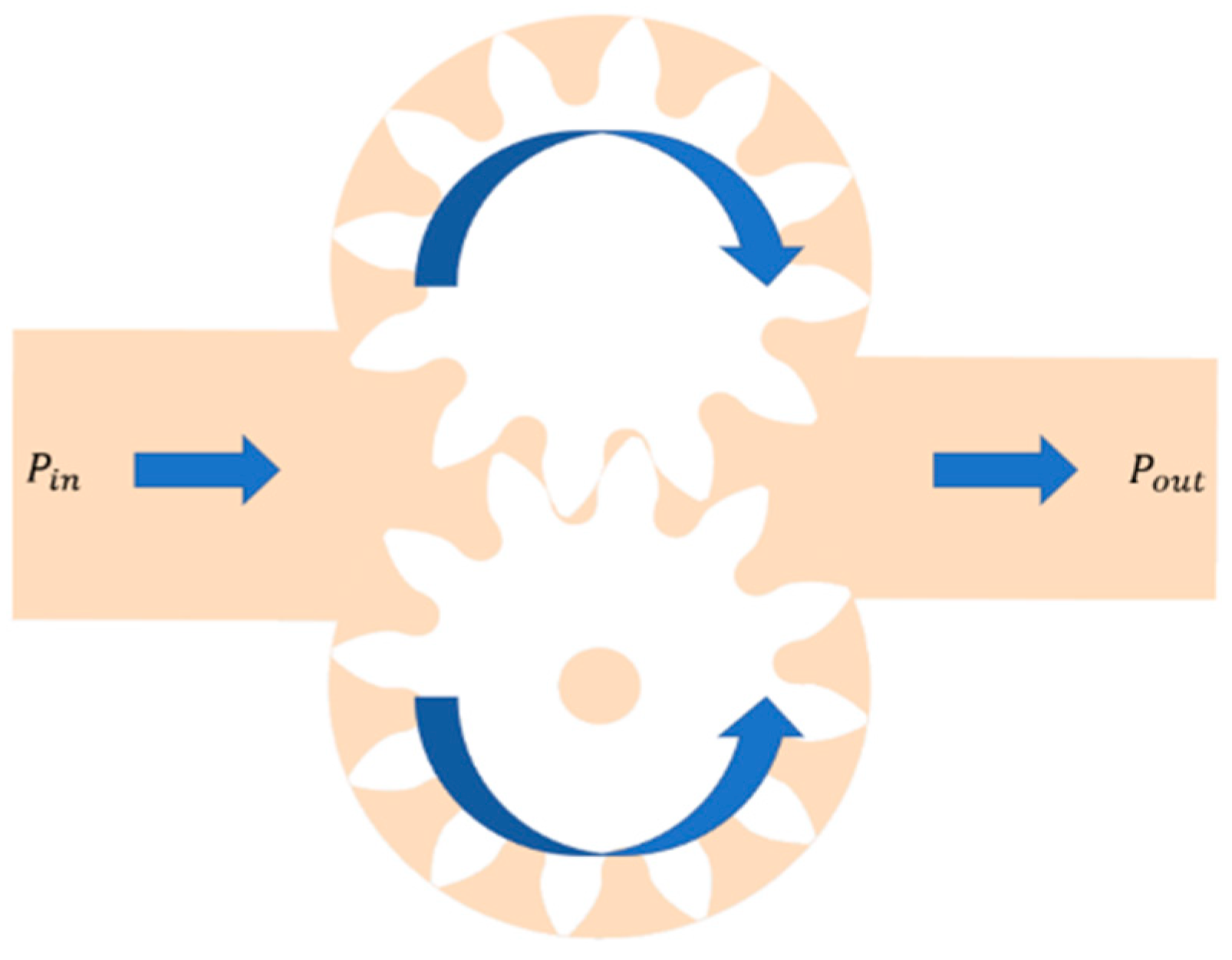
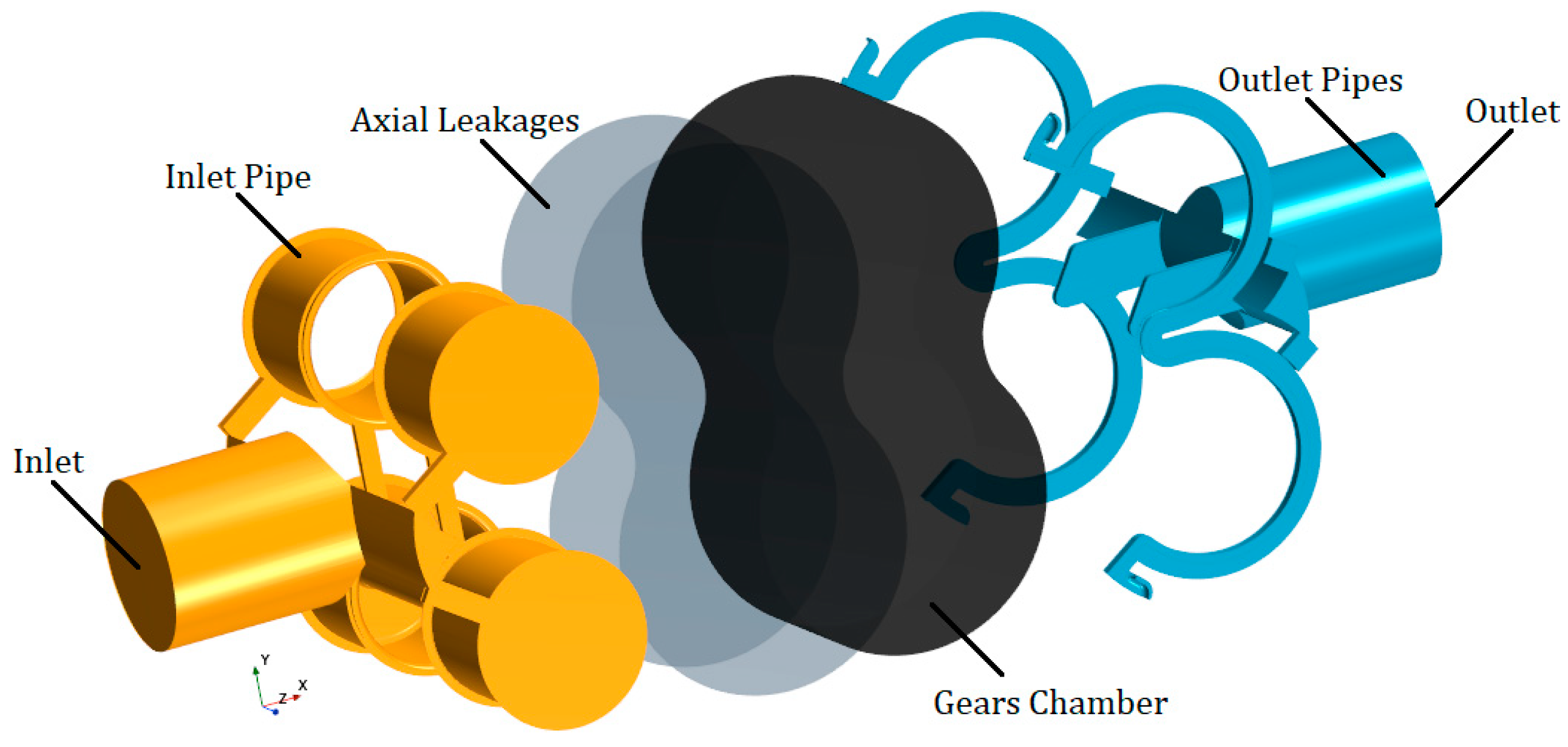
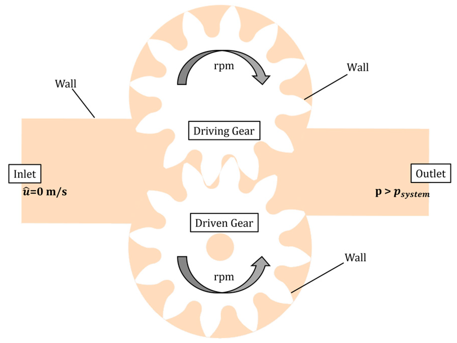
The 12-tooth external gear pump analyzed in the present study is simplified in its complex geometry as are both the overset and dynamic mesh cases. Figure 1 shows a section of the simplified EGP, the rotation directions of both the driving (upper) and driven (lower) gears and the flow path, highlighted with the subscript “in” on the left, indicating the inlet pressure, and the superscript “out”, indicating the outlet pressure. The fluid region was extracted from a 3D CAD model of an existing pump. This was further subdivided into different regions so that the meshing process could be more detailed and precise. This is a detrimental passage, which allows for specific zones that may require a higher focus during the mesh generation can be treated as necessary, i.e., leakages, motion regions, narrow sections, etc. As a general approach, the fluid region in an EGP can be split into two main fluid categories: the stationary and the moving regions. In Figure 2, the computational regions are reported with orange, blue and grey indicating the stationary part and the gear chamber as the only motion region.
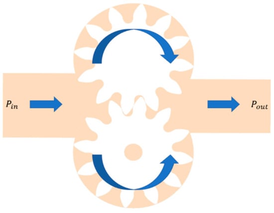
Figure 1.
Geometry section.

Figure 2.
Computational fluid regions.
The two meshing methods that are used in this study require a different treatment of the gear chamber. The overset mesh requires the existence of a background mesh and one or more overset meshes. For the present case, the background mesh will serve as a background region and two offset bodies obtained from the gears’ boundaries will be the two overset meshes. Since the overlapping region between the two overset meshes is small enough, there is no need to particularly extend the offset boundaries, so it was chosen to extend a little over the radial perimeter to ensure that the volumes are fully contained with the overset mesh while moving along the walls. As visible in Figure 3, the overset regions, in blue and pink, overlap each other following the rotation, from the high- to the low-pressure region, and then they overlap and exceed in extension the borders of the gear chamber, in grey in the picture, for a total of 1mm of offset from the original gears’ perimeter.
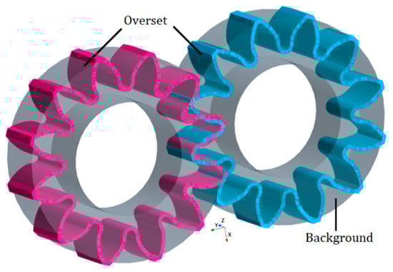
Figure 3.
Overset regions.
Inherently, in the dynamic mesh case, the moving region consists of a unique body. Here, the movement will be assigned to the gear boundaries and updated with each predefined rotation angle. To realize this volume, a simple volumetric subtraction of the gear bodies from the gears chamber’s internal volume is performed. In the dynamic case, the contact cannot be simulated, so proper clearance is needed in order to simulate the gear movement. Since distancing the gears would shorten the radial clearance, the gear case must be modified so that these clearances remain unaltered, and the volumetric efficiency is less affected.
In Figure 4, the dynamic meshing motion region is shown. Here, the gap between the gears in the contact zone is highlighted. The choice of the gap dimension depends on two main factors: the stability of the mesh and the volumetric efficiency loss. The first leads to higher numerical instabilities with smaller gaps, while the second behaves oppositely, with less efficiency loss with smaller gaps. Given these two factors, the choice falls forcedly in between the two, where the gap must be as small as possible to limit the volumetric efficiency loss but big enough for the mesh to remain topologically valid during the rotation.
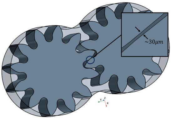
Figure 4.
Morphing motion region.
5. Mesh Settings
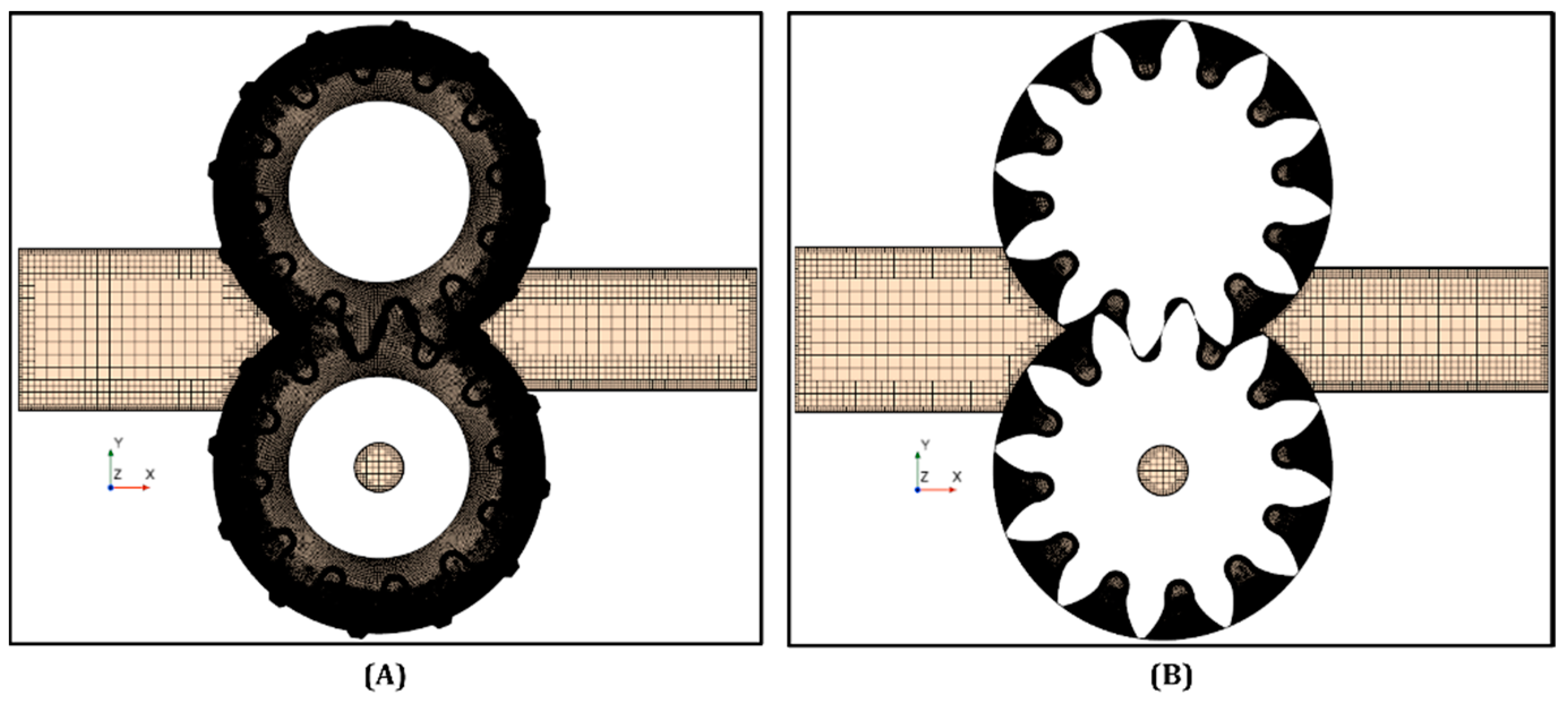
The overset mesh method and the dynamic/morphing method are used and compared in this study. For the generation of the base meshes, two approaches were used for both the overset and the morphing. For the motion region, being the overset regions and the background or the morphing region and the axial leakages, the directed mesh approach was used. As can be seen in Figure 3 and Figure 4, the regions are characterized by two surfaces with faces on the same plane, i.e., the gear sides and a regular depth linking the two sides of the regions. In this way, a base mesh can be generated on one of the lateral surfaces with relative custom operations, like proper refinements on the gear walls and the radial perimeter of the case. Then, the swept of the mesh, in order to generate perfectly regular cell layers, is generated along the depth dimension, i.e., the z-axis as reported in Figure 3 and Figure 4. For the pipes, the automated mesh was used since the complex geometry would not allow for a regular sweep along a direction. The overset mesh method is an exclusive feature of Simcenter STAR-CCM+, and it is based on the definition of donor (overset) and acceptor (background) cells in overlapping regions, with a selective activation/deactivation of cells in the overlap zone, referred to as hole-cutting. The hole-cutting process is shown in Figure 5, where a section of the whole geometry is reported before and after the initialization of the mesh.
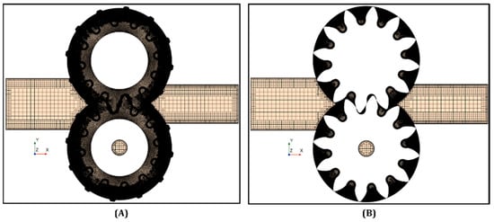
Figure 5.
Overset mesh (A) before and (B) after the initialization.
This motion requires the presence of a background region and an overset region, the former surrounding the moving objects, as can be seen in Figure 3. In the case of an EGP, the background region comprises the whole of the gear case, and the overset regions are defined so that they fully encompass the two gears. As already mentioned in C, the overset regions were obtained by offsetting the perimeter of each gear. The offset dimension was set as 1 mm in order to restrict the overset region as much as possible since its meshing affects the computational expense of the calculation. With the given dimension, the extension of the overset region is enough to encompass the radial leakages while the gears rotate and the contact points immediate surroundings. The overset mesh technique then allows the simulation of the contact point by deactivating cells when opposing walls are within a certain distance; in the present case, this happens when the two walls are in contact. The motion of the gears is defined in Simcenter STAR-CCM+ as a rigid rotation about a given axis. As the gears rotate, the cells in the gear contact region are dynamically activated and deactivated.
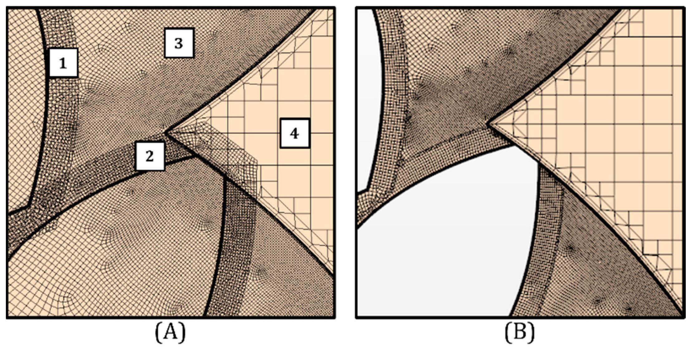
Figure 6 shows the hole-cutting process in detail for the outlet section of the high-pressure zone with the same orientation as in Figure 5. In Figure 6A, all the elements are meshed. Those are the outlet pipe conduit on the right (4), easily detachable by the coarser mesh; the background region (3), characterized by a finer mesh with refinement in correspondence with the outlet pipe interface and then the overset meshes (1–2), which, with a higher refinement, surround the gears teeth profiles. Before the initialization, all of the cells are visible, and the overset meshes overlap with the others. Once the mesh is initialized, only the appropriate cells are active and visible, resulting in the correct volume being available for the fluid, where the gear boundaries are now identifiable as moving walls. This process of activation/deactivation is triggered by the donor (overset) cells once they overlap with the acceptor (background) cells. When the cells overlap, the background cells are deactivated, and the solution is interpolated with the remaining cells, as shown in Figure 6. Then, if the donor cells go out of boundaries, as in the case of the radial perimeter of the gears chamber, or alternatively, overlap with cells that are not marked as acceptors (as for the pipes cells), then these cells are simply inactivated, as shown in Figure 5, where the section covers all the gear pump extension, or in Figure 7, where the detail is focused on the external perimeter in the lower part of the geometry, for the same orientation as in Figure 5. Here, the overset part that surrounds the tip of the gear tooth when meeting the external surroundings of the geometry is totally inactivated and confined to the radial leakage between the tip and the gear chamber wall.
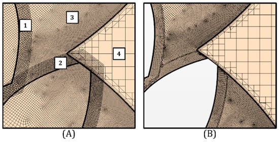
Figure 6.
Overset mesh section before (A) and after initialization (B) in correspondence to the high-pressure zone.
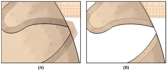
Figure 7.
Overset mesh section in the peripherical region before (A) and after (B) initialization.
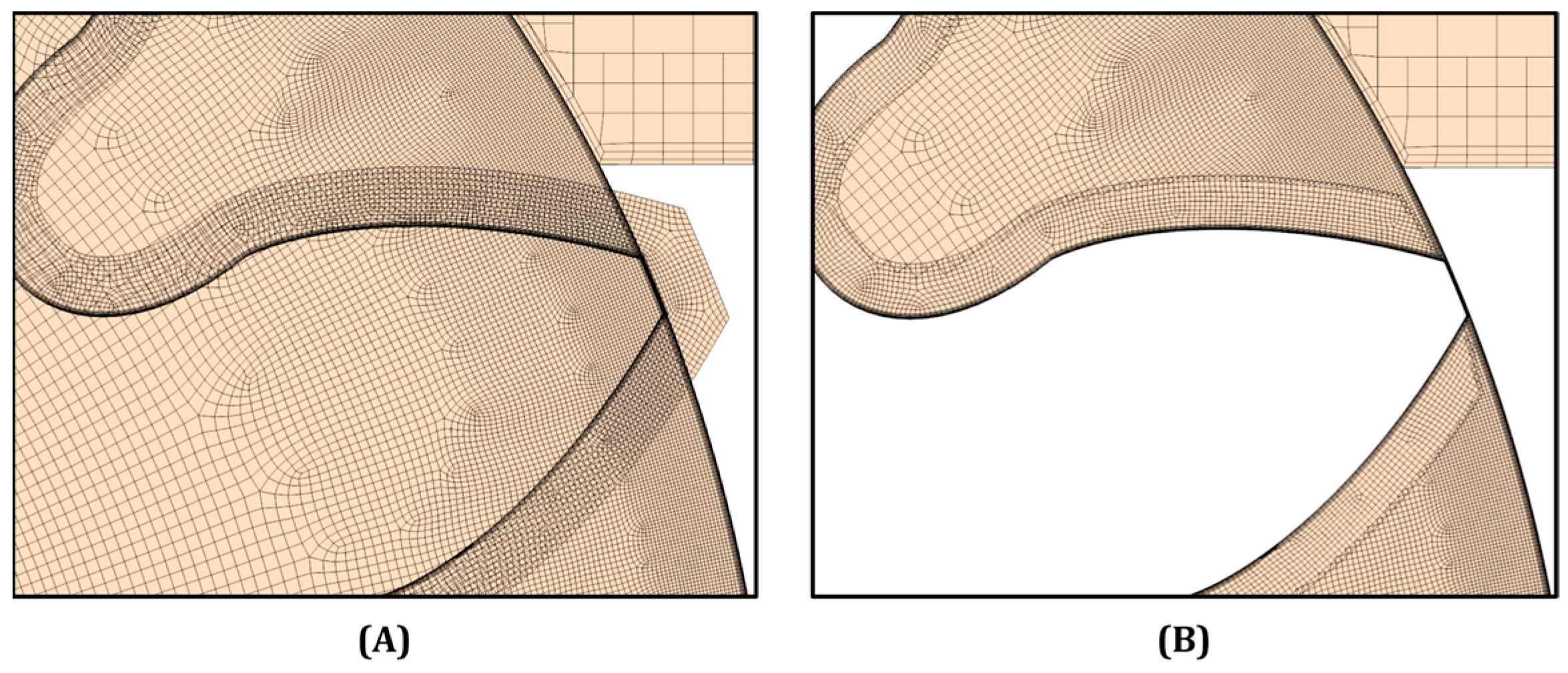
Different from the overset method, the dynamic method does not require a hole-cutting process. The workflow logic is based on a gradual distortion of the mesh by rotating the gears walls. Obviously, a single mesh generated for a specific geometric topology cannot hold a continuous movement of the boundary walls for it leads to a consequent distortion of the cells’ topology. If the distortion is too high, then the cells become topologically invalid, and the calculation stops. Then, to avoid this problem, just a certain amount of distortion of the cells will be obtained with a defined quantity of motion in the boundary walls. Another important element is the dimension of the cells in the generated meshes. Different from the overset mesh within the morphing method, all is based upon the structural integrity of the mesh cells. The smaller the cells, the quicker the distortion for wider degrees of rotation. So, the dimension of the cells directly affects the amplitude of the single timestep. For the morphing method, then it is possible to make use of a coarser mesh, as clearly visible in Figure 8, also relying on the existence of a continuous gap between the gear teeth, as shown in Figure 8B with means of the arrow. The generation of the mesh also takes into account the relationship between the cell dimension and the timestep amplitude, i.e., the rotation degree. This was chosen so that the single timestep did not have to remain too small, which would have slowed down the whole calculation.
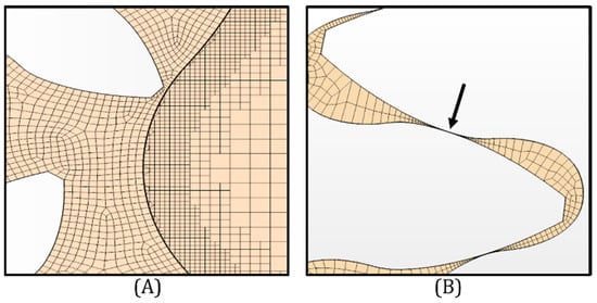
Figure 8.
Dynamic mesh section details of the outlet pipe (A) and the gear non-zero contact point (B).
Once the prefixed cell distortion limit is reached, another mesh is generated in that same topology and the process starts over again. Fortunately, this process of generating new meshes does not need to be performed for a full revolution of the gears. Given the repetition of the motion (for each 30°), a limited number of meshes can be generated before the calculation and then updated when the topology requires a mesh change. For this case, an initial mesh was generated with a coarser topology than the overset mesh, and each subsequent mesh was used to cover 2° of rotation. By doing so, the total number of meshes that was obtained was 15. In fact, the total amount of covered degrees for the 15 meshes with 2° each is precisely 30°, which is the repetition of the motion for this kind of pump.
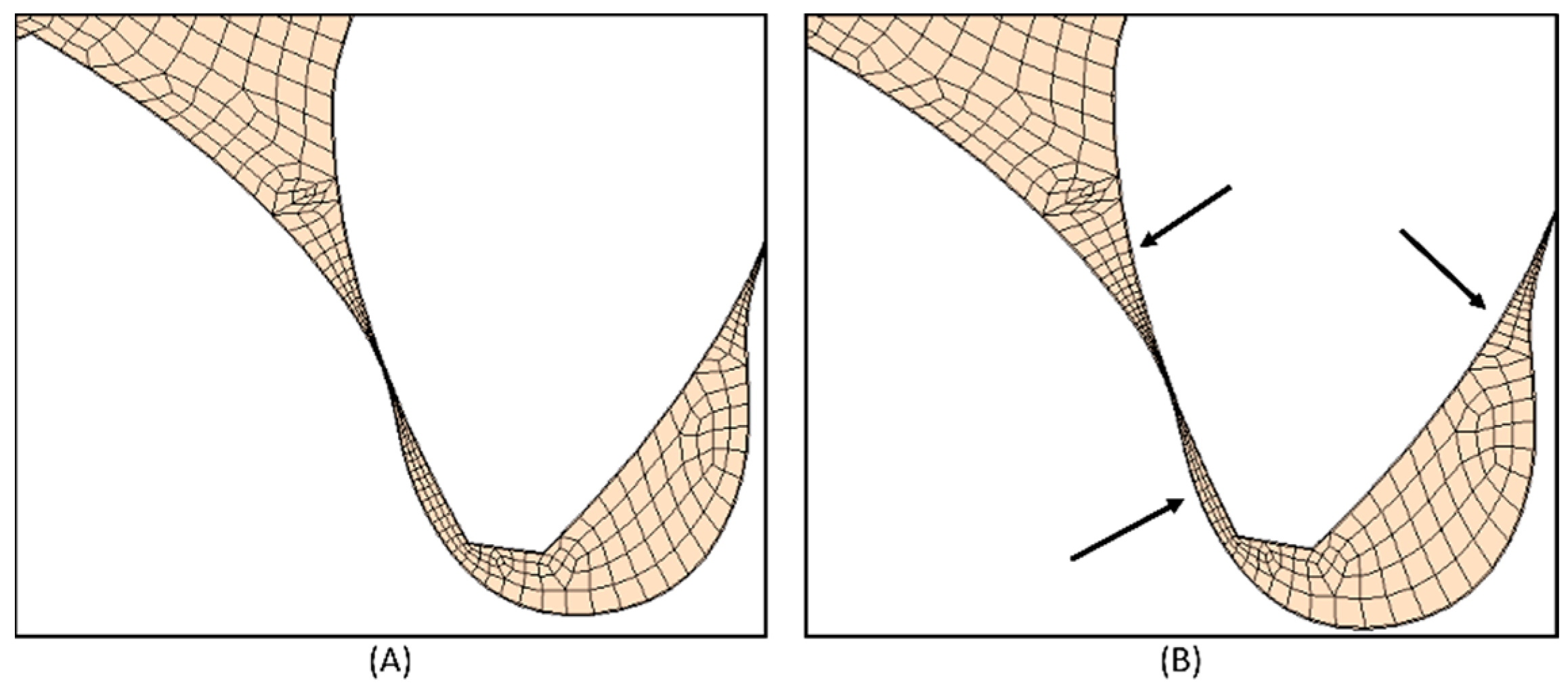
In Figure 9, two different moments of the rotation of a mesh are reported. In Figure 9A, the initial positions of the gear teeth are shown, and the cells are as immediately generated with the mesher. In Figure 9B, the last timestep is shown, which is after 0.25° of rotation. It can be noticed that the distortion is not particularly evident. The distortion can be seen as a compression in correspondence with the engagement of the teeth profiles, as pointed out with the lower arrow. Coherently with the rotation dynamic, each gear’s approach is preceded and followed by a distancing, so the upper arrows point to where the cells are stretched in the given image. After Figure 9B, the mesh is updated with a new one generated in the same position, which will be rotated for another 0.25° of rotation. The small degree of distortion is defined to ensure the stability of the mesh. It is important to note that the degrees of stability of one mesh are not necessarily the same for the others. Since the morphing methodology allows for the use of a coarser mesh with respect to the overset, the use of a smaller timestep combined with the higher calculation velocity is reasonable.

Figure 9.
Dynamic mesh sections for (A) starting position and (B) final position after 0.25° of rotation.
In Figure 10, both the overset and dynamic mesh workflows are shown. For the dynamic mesh methodology, it is also important to specify the use of a new feature in STAR-CCM+, which is the solution interpolation. This new feature is specifically created in order to correctly interpolate one solution to the other mesh and fill, with a mass source, the unavoidable mass gap that interpolation itself creates. This is externally handled using Java code that executes the whole dynamic method. These two techniques are completely different in many aspects, as briefly listed in Table 1 and explained below:
- Methodology implementation: the overset is fully integrated into STAR-CCM+, while the dynamic requires external Java code in order to execute the entire workflow.
- The number of pre- and working meshes: the overset mesh relies on two different mesh types for the motion region, which, in the present case, are two overset meshes (master and slave) generated along the gear profiles, and a background mesh that covers the entire motion region. Then, during the calculation, these three meshes constantly interact and work as one single mesh. In the dynamic method, one single mesh is required in the motion region, which is generated in the gear chamber, where the gear profiles were already subtracted, and the motion is defined on the internal walls obtained with the gear profiles. Then, in the present case, the 15 meshes obtained for each 2° of rotation are needed for the ongoing simulation.
- Refinement of the mesh: the overset mesh being deputed to the resolution of the zero-contact point needs a high refinement in the overset meshes so that approaching the zero-contact point can be resolved with enough numerical precision, which also leads to higher numerical stability. The dynamic mesh then permits the use of coarser meshes, with a certain refinement in correspondence with the gears’ leakage, which must maintain sufficient topological stability while covering the assigned rotation degrees.
- Zero contact point resolution: the overset mesh with the hole-cutting process is able to simulate the existence of a zero-contact point when the gear walls come in contact. On the other hand, the dynamic mesh is not able to hold the formation of a zero-contact point as it would require the complete compression of one or more cells in between the cells.

Figure 10.
Meshing workflow for (A) overset and (B) morphing.
Figure 10.
Meshing workflow for (A) overset and (B) morphing.
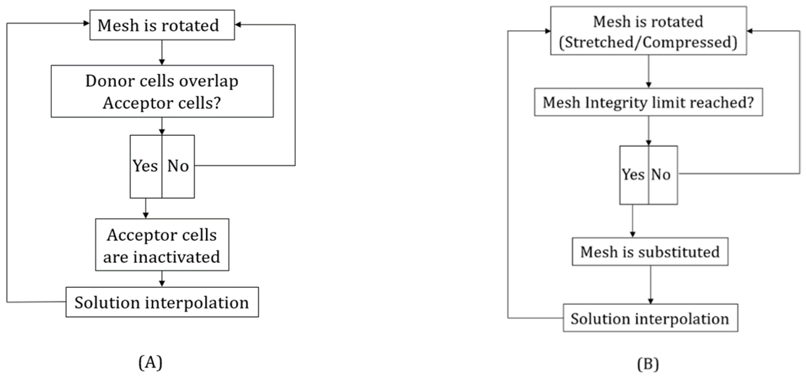

Table 1.
Overset and dynamic mesh methods main differences.
Table 1.
Overset and dynamic mesh methods main differences.
| Code | Regions | Contact | Meshes | |
|---|---|---|---|---|
| Overset | No | 3 | Yes | 1 |
| Dynamic | Yes | 1 | No | 15 |
The last main difference of the dynamicmethod is the implementation of a new feature in STAR-CCM+ called solution interpolation, which is specifically created to correctly interpolate data from one mesh to another and to fill, with a mass source, the unavoidable mass gap that the interpolation generates. An external code is created in the Java language in order to control the meshing substitution process, which represents the main difference between this method and the overset method, which does not require any external code to run. When the calculations with the overset mesh were performed, this method was not already implemented in STAR-CCM+, and the overset mesh method did not feature it. However, it is now at the disposal of every meshing method that the user may use, which will surely improve the continuity equation solution and the numerical stability of the calculation.
Inherently, the mesh dimensions for the overset method, in order to stabilize the calculation, a very fine mesh is required for the motion region, i.e., where the three meshes interpolate each other. For the background mesh, a base size of 2 × 10⁻⁴ m was chosen. For each overset mesh, a finer mesh was generated with a base cell size of 9 × 10⁻⁵ m. For both the background mesh and the overset mesh, eight prism layers were sufficient to resolve the near-wall velocity, while the swept number of layers in the transversal direction was set to 75. The mesh generated with such parameters led to 34 M cells. As already mentioned, the dynamic mesh was generated using a coarser mesh. The motion region, being composed of a body alone, used the directed mesh, where one lateral side was used to generate a classic surface mesh with a base size of 2.0 mm. The depth direction was used to sweep the surface mesh along a defined number of layers, which was chosen to be 50, most likely generating regular-shaped cells. This led to a total of approximately 3 M cells. This highlights the difference between the two methods regarding the computational effort required to stabilize the calculation.
6. Simulation Parameters
The system was simulated starting at rest with the fluid at and the gears still with . The boundary conditions of the system are shown in Figure 11, where the same section as in Figure 1 is reported with the addition of the boundary conditions as they were set for both simulations. As reported, the inlet was set as a stagnation inlet, which means that the fluid is considered at rest, and its movement depends on the “suction” effect driven by the system. During the simulation, both the driven and the driving gears are moved by the definition of motion, with respect to the reference axis centered in the center of the gears, by the prescribed . In this case, the same value was set for both gears, and the longitudinal axis direction was +z for the driven gear and −z for the driving gear. The outlet was defined as a pressure outlet with a pressure value higher than the pressure in the system. In this way, the pressure outlet simulates the rest of the subsequent hydraulic circuit with its suction effect. For a 3D reference for the inlet and the outlet position, Figure 2 can be considered. The velocity and pressure fields were resolved using a SIMPLE algorithm of the second order. For the turbulence methods, both the and the a second-order convection scheme was used. Then, the timescale was resolved using an implicit unsteady algorithm of the first order. For the dynamic method, a timestep corresponding to a 0.25° of rotation was given, while for the overset, the timestep was set to correspond to 1° of rotation. The results were collected for the last complete rotation cycle after the solution reached a computational stationary behavior; in this case, corresponding to the results of the fourth complete cycle.
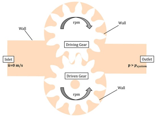
Figure 11.
Boundary Conditions for the simulations.
7. Results
The results from the fourth and last simulation cycle, in which both simulations attained cyclic conditions, are presented. A comparison is made between the mass flow averaged outlet pressure, the outlet flow rate, and the vane pressure measured using a single-point probe. Then, as mentioned in the cavitation account section, contour scenes of the pressure intervals corresponding to the aeration and cavitation phenomena are presented in order to make a comparison in terms of their extension and localization.
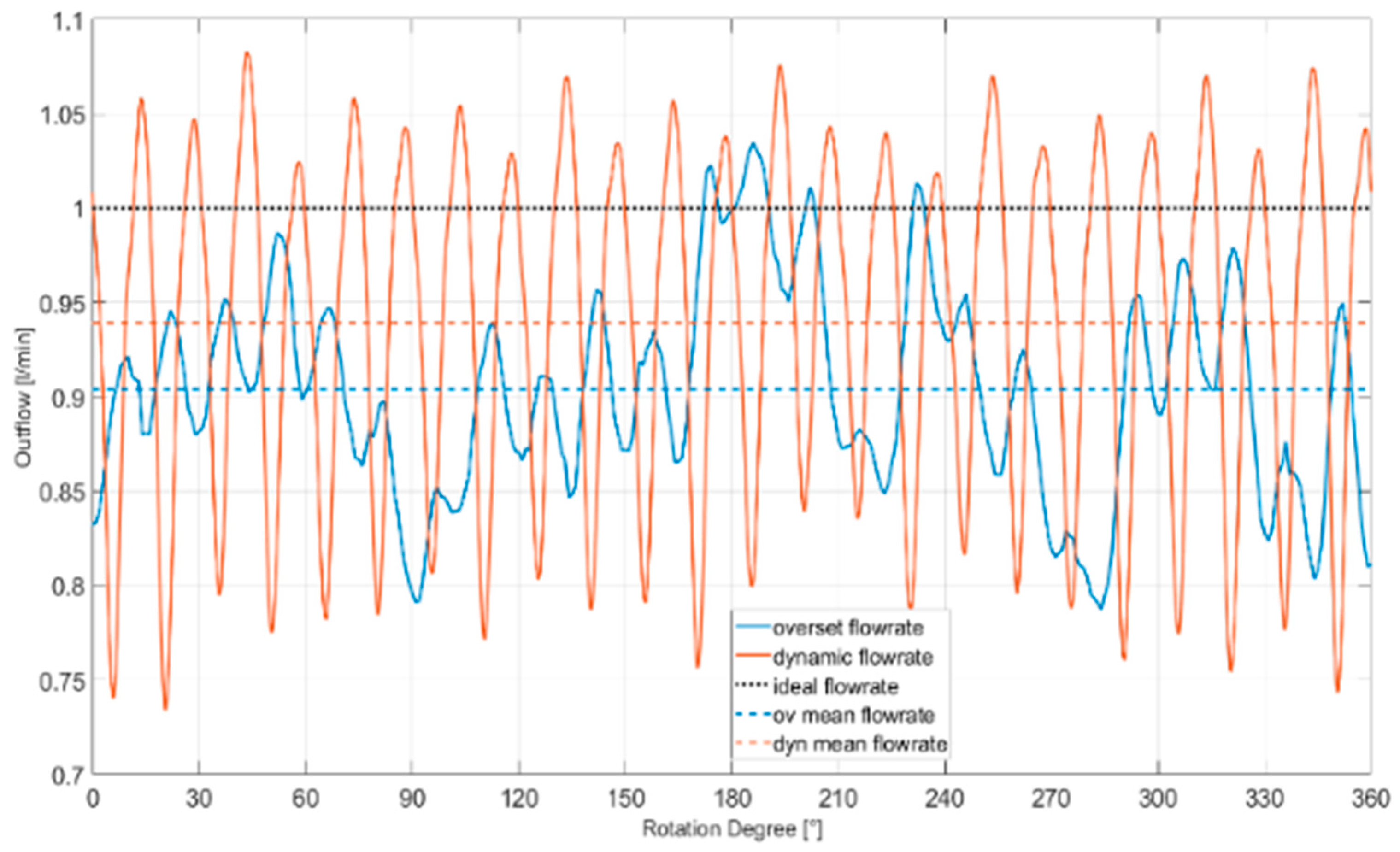
In Figure 12, the outflow rates for the two meshing methods are reported. The black dotted line reports, the theoretically elaborated flow rate, calculated as , where is the volumetric displacement and is the rotation regime. Its value was normalized to 1, and the mean flow rates for the two meshing methods were normalized on this value. For the totality of a complete rotation, the instantaneous flow rates are reported, and it can be seen that the dynamic values (orange) are characterized by wider oscillations when compared with the overset (blue) values. In addition, the peaks in the overset mesh tend to anticipate their correspondents in the dynamic mesh. The dashed lines represent the mean value of the overall flow rate during the complete cycle, which is useful to make a comparison between the two settings. Considering the mean values are both lower than the theoretical one, as expected, the dynamic elaborates a higher flow rate than the overset one, with a difference of less than ~5% between the two flow rates, with less than a 10% for the overset and less than 7% for the dynamic with respect to the theoretical flow rate. Given the data presented by the authors, this is a direct comparison and validation with respect to the effective machine, considered in this case as the ideal scenario.
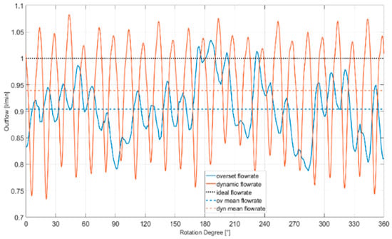
Figure 12.
Outflows plot.
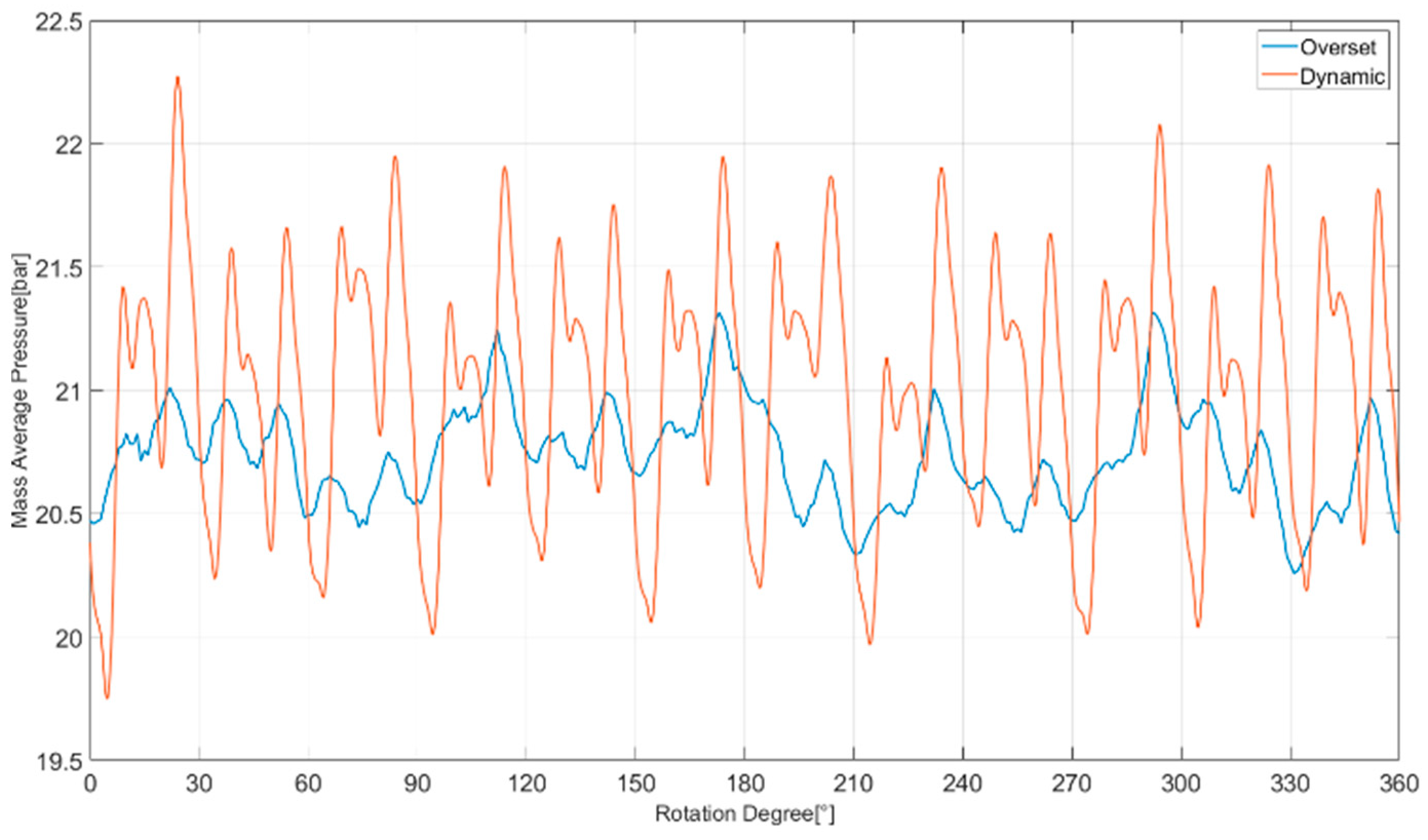
In Figure 13, the mass flow average pressures at the outlet sections are reported. These were calculated using an average based on the oil mass flowing through the outlet section, where the pressure was calculated at each predefined timestep. The pressure ripples depend on the continuous opening of the radial teeth closed volumes. These can be seen to be wider in amplitude for the dynamic case with respect to the overset, with an oscillation between 20 to 22 bar and a narrower interval for the overset mesh between 21.5 and 20.25 bar. These results show that for the overset mesh method, the fluid undergoes a more stable behavior. For the dynamic mesh method, the presence of so many ripples wider in amplitude shows that the fluid undergoes a more disturbed flowing to the outlet. The difference between the two meshing methods in this case can be related to the existence of the continuous leakage between the teeth in the contact zone. The presence of the leakage leads to a continuous flowing of oil through it, which leads to an additional disturbance of the mean flow, and thus the related physical quantities. Figure 10 perfectly shows the effect of a continuous leakage if existent in between the gear teeth in the meshing region, which leads to a higher disturbance of the flow that is evidenced by the higher and more frequent peaks in pressure measured at the outlet section.
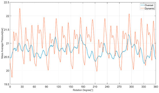
Figure 13.
Outlet mass flow average pressure plot.
Figure 14 reports the pressure in correspondence with a probe is realized so that it will rotate along the driving gear. Doing so, it is possible to monitor the pressure varying in the hollow between two teeth so that once the gearing happens, regarding the generation of the “enclosure”, its opening to the inlet region and the progression along the external perimeter of the gears chamber can be monitored in full. Following the overset pressure vane line (blue), it can be observed that starting from the point indicated in the section, with the engagement already created, the pressure starts rising to the maximum value and then starts to lower while the point moves toward the disengaging to the lowest point once the enclosure is completely opened to the low-pressure region of the inlet. Then, moving along the perimeter of the gear chamber, the pressure rises gradually as the point approaches the higher-pressure zone with a final quick ramp that is coherent with the opening of the hollow to the high-pressure region of the outlet. Within this monitor, the dynamic case shows its weakness, while in the comparison of the flow rates, it seems to provide better results. It is easily noticeable that the pressure presents a very different behavior. First of all, the pressure ramp runs out quicker and with a higher maximum value, according to the higher values reported in Figure 13. Then, the most evident difference resides in the values that are registered while the enclosure of the probe moves along the external perimeter of the gear chamber, where the pressure values remain quasi-totally still at zero. Then, the pressure abruptly arises when the enclosure is near the high-pressure region within a few angles. If inherently the flow rates at the outlets, the dynamic mesh method seems to lead to better results if compared to the overset meshing method, but when it comes to the pressure field, it is evident that the dynamic mesh method fails if compared to the overset. This may be due to two main distinctive characteristics of the two meshing methods. First, the dynamic mesh method maintains a continuous open passage in between the teeth so that the gear engagement in fact never happens, thus leading to a continuously flowing flow, which can be considered to be the main promoter of the wider pressure ripples. Second, the dynamic mesh method implements the solution interpolation, which limits the mass discontinuities between the interpolation of the fields from a mesh and the successive one. The overset mesh then does not present such an implementation, being a unique mesh assembly that works from the beginning to the end of the calculation. The usage of the overset mesh presents a weak point, while geometric variable leakages are present in the physical domain. The approaching of the teeth sides and their engagement leads to the inactivation of cells that may happen where, due to the non-excessive refinement in those points not weighing down, the engaging/disengaging is gradually generated. The fact that those inactivated cells are unavoidable leads to a discontinuity in the flow characteristic fields that is most probably the main source for the lower instantaneous and mean flow rates.
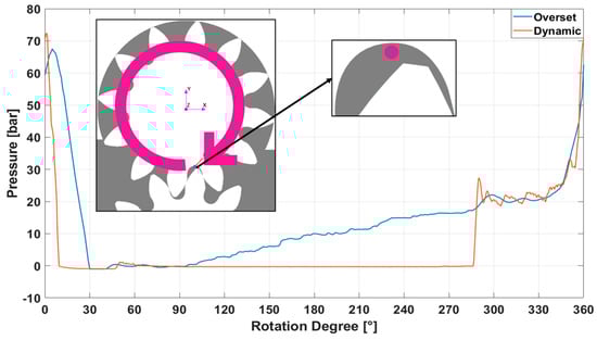
Figure 14.
Pressure in the vane along a cycle.
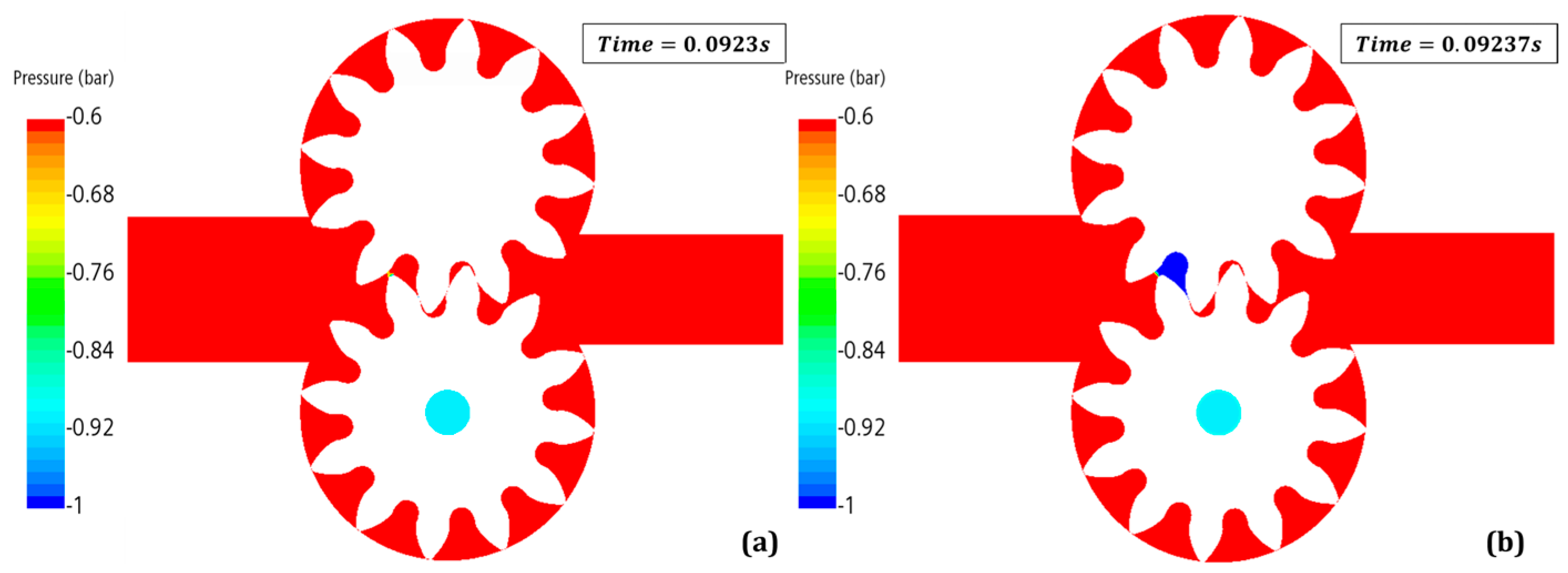
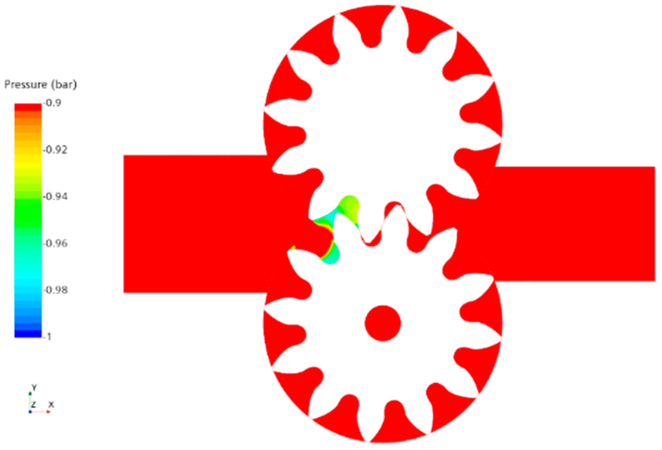
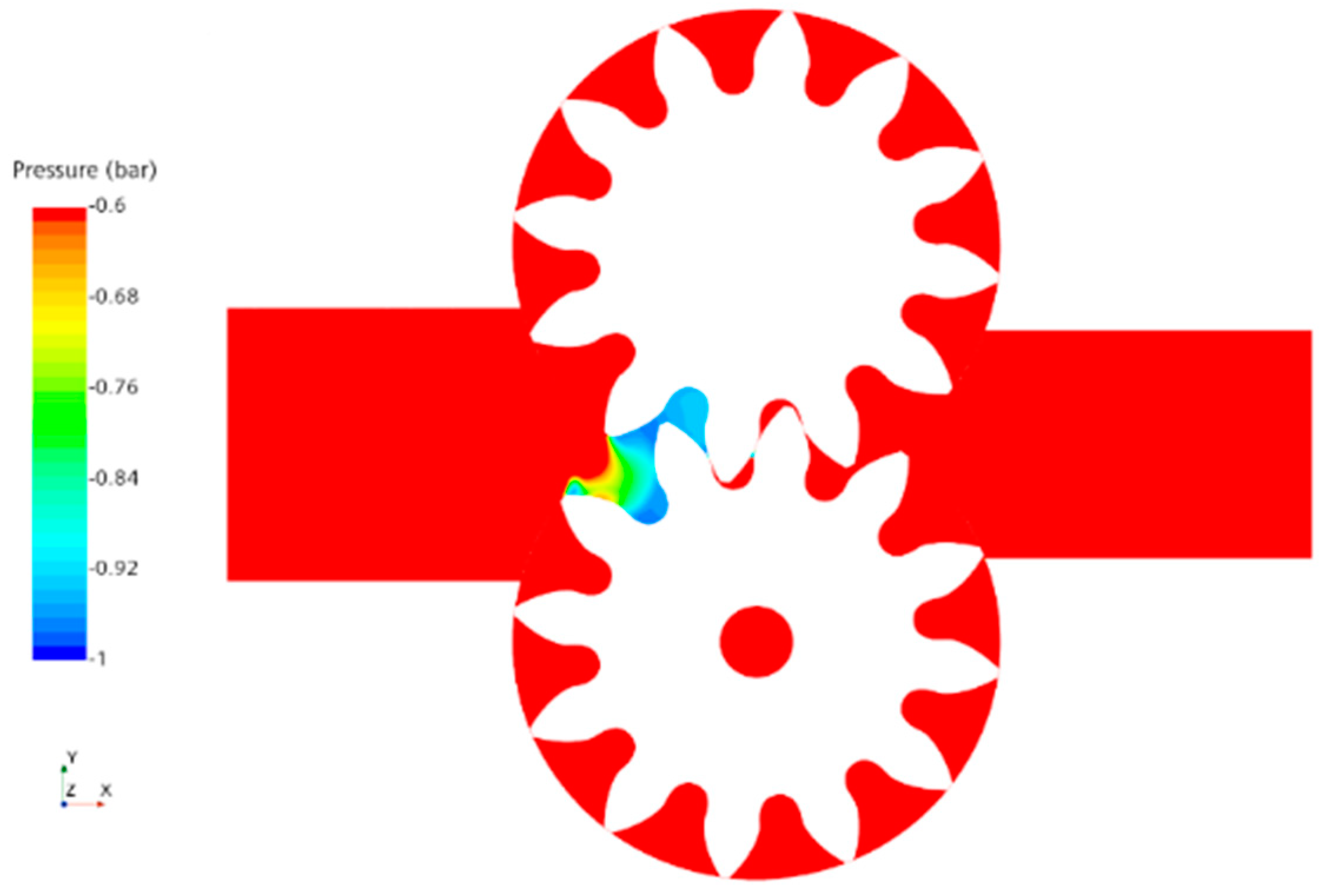
Finally, acknowledging the characteristics of the MultiG, oil it is possible to define two ranges where cavitation and aeration generally take form, being [−0.9 bar; −1 bar] for cavitation and [−0.6 bar; −1 bar] for aeration. Plotting them in a contour scene for a section plane along the x–y axis leads to graphic evidence of the more probable regions where these phenomena may take form. In Figure 15 and Figure 16, the overset method results are reported for cavitation and aeration, respectively, while in Figure 17 and Figure 18, the same are reported for the dynamic method. For the overset results, two successive time frames at 0.0923 s and 0.09237 s are reported, and it is easily noticeable how at the end of the fourth cycle at 0.0923 s, both phenomena are suppressed within the whole pressure in the section of the system being higher than −0.6 bar. In the successive frames when the teeth disengage, the formation of a cloud of depression is evident where cavitation and aeration can appear, resulting in an evident effect due to the effective engaging of the teeth that leads to the formation of closed chambers, where the pressure drop happens once the leakage is created in correspondence to the region of low pressure in the inlet. For the dynamic mesh, just one time frame is reported at the end of the fourth cycle at 0.0923 s, in Figure 17 and Figure 18, and the appearance of a widespread region in the subsequent hollow is evident after the one that would be enclosed between the engaged teeth. Confronted to the overset scenes, the absence of a contact point result is evident in this graphic comparison for the generation of a wider region of negative values of pressure, which extends over the first opened chamber into the inlet region.
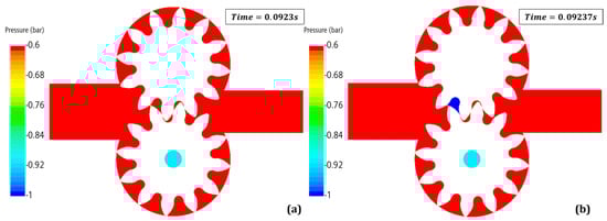
Figure 15.
Aeration pressure range contours for the overset method for two subsequent frames being (a) 0.0923 s and (b) 0.09237 s.
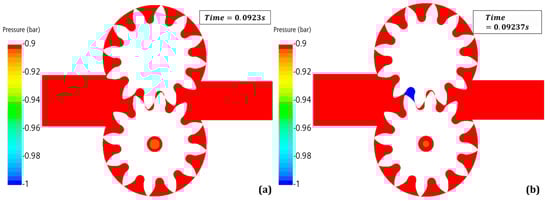
Figure 16.
Cavitation pressure range contours for the overset method for two subsequent frames being (a) 0.0923 s and (b) 0.09237 s.

Figure 17.
Cavitation pressure range for the dynamic method at 0.0923 s.

Figure 18.
Aeration pressure range for the dynamic method at 0.0923 s.
While in the overset frames, once the chamber opens, the depression region is characterized by a mean value next to −1 bar, resulting in an equally distributed region for both the pressure ranges. In the dynamic frames, the depression regions are characterized by different extensions based on the different ranges, with the aeration region being wider and spreading along the tooth of the driven gear facing toward the inlet region. This effect is easily related to the minimum leakage that, while not enclosing the teeth chambers during their engagement, leads to the pressure gradients that are easily observable in the images.
8. Conclusions
This paper presents a comparison between two meshing methodologies in the STAR-CCM+ environment, one being a well-consolidated technique in the CFD simulations of external gear pumps, usually named dynamic meshing, and the other being a meshing technique owned exclusively by STAR-CCM+. The dynamic methodology is unable to treat the contact point of these volumetric machines and is characterized by the continuous replacement of meshes, with the rotation of the gears and the solution interpolation between the mesh and the successive one, and it is also controlled by an external user code. The overset method is based on the overlapping of overset meshes, generated along the perimeter of the gears, between each other and a background mesh representing the gear chamber region. This method requires no replacement or interpolation or user code to be controlled. The comparison between the results of the two methodologies showed that the dynamic mesh, requiring solution interpolation, results in being more effective with regard to the outflow rate, where more oil is worked so that the mean flow is nearer to the theoretical flow rate elaborated by the pump, while the pressure ripples results in wider peaks if compared to the overset method. Both the pressure ripples and the outflow rates also result in a slight delay if compared to the ones of the overset method. Then, a comparison with means of a point probe positioned in a tooth hollow was reported, and the overset method was the only one capable to reproduce the pressure gradual rising along the progression of the probe from the low-pressure region of the inlet to the high-pressure region of the outlet. Finally, contours of the pressure range for the localization of cavitation and aeration phenomena were reported in a section along the x–y axis, reporting the effective impact of the simulation of a zero-contact point to the formation of a cavitation and aeration cloud. The dynamic method, which presents a continuous leakage between the teeth, leads to the formation of a depression cloud, while in the overset method, the results are suppressed due to the isolation of the enclosed chamber. In fact, the result for a successive frame is reported for the overset method, and once the contact fails, a depression cloud appears toward the inlet region. As a final summary of each method, it appears clear that neither of the two methods results in being absolutely better than the other. Thus, other in-depth studies will be performed in the future to investigate the registered fails of each method. Based on the results, the dynamic meshing method nevertheless presents more realistic results related to the general working of these machines. Those results are relative to the cavitation cloud, where the overset cavitation cloud results in a very confined and almost suppressed extension, and the mean oil flow rate, which is closer to the ideal flow rate of the machine. Therefore, considering the topic of the cavitation simulation in a CFD environment, the dynamic mesh method results, at the moment, as being preferable for use, specifically for STAR-CCM+, and for other numerical environments, it still results in being easier to apply.
Author Contributions
Conceptualization, F.O.; Methodology, G.M.; Supervision, M.M., F.P. and L.M. All authors have read and agreed to the published version of the manuscript.
Funding
This research received no external funding.
Data Availability Statement
Restrictions apply to the availability of these data.
Conflicts of Interest
The authors declare no conflict of interest.
References
- Strasser, W. CFD investigation of gear pump mixing using deforming/agglomerating mesh. J. Fluids Eng. Trans. ASME 2007, 129, 476–484. [Google Scholar] [CrossRef]
- Castilla, R.; Gamez-Montero, P.J.; Ertrk, N.; Vernet, A.; Coussirat, M.; Codina, E. Numerical simulation of turbulent flow in the suction chamber of a gearpump using deforming mesh and mesh replacement. Int. J. Mech. Sci. 2010, 52, 1334–1342. [Google Scholar] [CrossRef]
- Labaj, J.; Husar, S. Analysis of Gear Pump Designed for Manufacturing Processes. Appl. Mech. Mater. 2015, 803, 163–172. [Google Scholar] [CrossRef]
- Frosina, E.; Senatore, A.; Rigosi, M. Study of a high-pressure external gear pump with a computational fluid dynamic modeling approach. Energies 2017, 10, 1113. [Google Scholar] [CrossRef]
- Corvaglia, A.; Rundo, M.; Casoli, P.; Lettini, A. Evaluation of tooth space pressure and incomplete filling in external gear pumps by means of three-dimensional cfd simulations. Energies 2021, 14, 342. [Google Scholar] [CrossRef]
- Casari, N.; Fadiga, E.; Pinelli, M.; Randi, S.; Suman, A. Pressure pulsation and cavitation phenomena in a micro-ORC system. Energies 2019, 12, 2186. [Google Scholar] [CrossRef]
- Yoon, Y.; Park, B.H.; Shim, J.; Han, Y.O.; Hong, B.J.; Yun, S.H. Numerical simulation of three-dimensional external gear pump using immersed solid method. Appl. Therm. Eng. 2017, 118, 539–550. [Google Scholar] [CrossRef]
- Del Campo, D.; Castilla, R.; Raush, G.A.; Montero, P.J.G.; Codina, E. Numerical analysis of external gear pumps including cavitation. J. Fluids Eng. Trans. ASME 2012, 134, 081105. [Google Scholar] [CrossRef]
- Star-CCM+ Software. 2022. Available online: https://www.plm.automation.siemens.com/global/it/products/simcenter/STAR-CCM.html (accessed on 19 July 2023).
- Milani, M.; Montorsi, L.; Muzzioli, G.; Storchi, G.; Terzi, S.; Rinaldi, P.P.; Stefani, M. Numerical and experimental analysis of a novel concept for axels dry braking system in off-road vehicles. In ASME International Mechanical Engineering Congress and Exposition; American Society of Mechanical Engineers: New York, NY, USA, 2020; pp. 1–7. [Google Scholar] [CrossRef]
- Muzzioli, G.; Paini, G.; Denti, F.; Paltrinieri, F.; Montorsi, L.; Milani, M. A lumped parameter and CFD combined approach for the lubrication analysis of a helical gear transmission. J. Phys. Conf. Ser. 2022, 2385, 012034. [Google Scholar] [CrossRef]
- Muzzioli, G.; Montorsi, L.; Polito, A.; Lucchi, A.; Sassi, A.; Milani, M. About the influence of eco-friendly fluids on the performance of an external gear pump. Energies 2021, 14, 799. [Google Scholar] [CrossRef]
- Menter, F.R. Two-equation eddy-viscosity turbulence models for engineering applications. AIAA J. 1994, 32, 1598–1605. [Google Scholar] [CrossRef]
- Menter, F.R. Instationär Kavitierende Strömungen—Ein Neues Modell, Basierend auf Front Capturing (VoF) und Blasendynamik. Ph.D. Thesis, The Karlsruhe Institute of Technology, Karlsruhe, Germany, 2000. [Google Scholar] [CrossRef]
- Siemens PLM Software. Star-CCM+ 17.02.007 User Guide; Siemens PLM Software: Plano, TX, USA, 2022. [Google Scholar]
- Jiang, Y.; Furmanczyk, M.; Lowry, S.; Zhang, D.; Perng, C.Y. A Three-Dimensional Design Tool for Crescent Oil Pumps; No. 2008-01-0003 SAE Tech. Pap.; SAE: Warrendale, PA, USA, 2008. [Google Scholar]
- Ruvalcaba, M.A.; Hu, X. Gerotor fuel pump performance and leakage study. In Proceedings of the ASME International Mechanical Engineering Congress and Exposition, Denver, CO, USA, 11–17 November 2011; pp. 807–815. [Google Scholar]
- Frosina, E.; Senatore, A.; Buono, D.; Manganelli, M.U.; Olivetti, M. A tridimensional CFD analysis of the oil pump of an high performance motorbike engine. Energy Procedia 2014, 45, 938–948. [Google Scholar] [CrossRef]
- Močilan, M.; Husár, Š.; Labaj, J.; Žmindák, M. Non-stationary CFD simulation of a gear pump. Procedia Eng. 2017, 177, 532–539. [Google Scholar] [CrossRef]
- Zhao, X.; Vacca, A.; Dhar, S. Numerical modeling of a helical external gear pump with continuous-contact gear profile: A comparison between a lumped-parameter and a 3D CFD approach of simulation. In Fluid Power Systems Technology; American Society of Mechanical Engineers: New York, NY, USA, 2018; p. V001T01A053. [Google Scholar]
- Shih, T.-H.; Liou, W.W.; Shabbir, A.; Yang, Z.; Zhu, J. A New Kt Eddy Viscosity Model for High: Reynolds Number Turbulent Flows. Comput. Fluids 1995, 24, 227–238. [Google Scholar] [CrossRef]
- Singhal, A.K.; Athavale, M.M.; Li, H.; Jiang, Y. Mathematical Basis and Validation of the Full Cavitation Model. J. Fluids Eng. 2002, 124, 617–624. [Google Scholar] [CrossRef]
- Schnerr, G.H.; Sauer, J. Unsteady cavitating flow—A new cavitation model based on a modified front capturing method and bubble dynamics. Am. Soc. Mech. Eng. Fluids Eng. Div. FED 2000, 251, 1073–1079. [Google Scholar]
- Schnerr, G.H.; Sauer, J. Physical and Numerical Modeling of Unsteady. In Proceedings of the Fourth International Conference on Multiphase Flow, New Orleans, LA, USA, 27 May–1 June 2001; pp. 1–12. [Google Scholar]


Disclaimer/Publisher’s Note: The statements, opinions and data contained in all publications are solely those of the individual author(s) and contributor(s) and not of MDPI and/or the editor(s). MDPI and/or the editor(s) disclaim responsibility for any injury to people or property resulting from any ideas, methods, instructions or products referred to in the content. |
© 2023 by the authors. Licensee MDPI, Basel, Switzerland. This article is an open access article distributed under the terms and conditions of the Creative Commons Attribution (CC BY) license (https://creativecommons.org/licenses/by/4.0/).