Abstract
We present an open-source code, Xyst, intended for the simulation of complex-geometry 3D compressible flows. The software implementation facilitates the effective use of the largest distributed-memory machines, combining data-, and task-parallelism on top of the Charm++ runtime system. Charm++’s execution model is asynchronous by default, allowing arbitrary overlap of computation and communication. Built-in automatic load balancing enables redistribution of arbitrarily heterogeneous computational load based on real-time CPU load measurement at negligible cost. The runtime system also features automatic checkpointing, fault tolerance, resilience against hardware failure, and supports power- and energy-aware computation. We verify and validate the numerical method and demonstrate the benefits of automatic load balancing for irregular workloads.
1. Motivation and Significance
We are developing an open-source software tool, Xyst, (https://xyst.cc, accessed on 27 March 2023), for large-scale computational fluid dynamics on top of the adaptive runtime system, Charm++ (http://charmplusplus.org, accessed on 27 March 2023). Our target application areas include aerodynamics and flows around buildings with complex structures, e.g., in urban environments. Common features of these problems are flow around complex 3D geometries and large variations in length scales that must be accurately resolved. This requires computational meshes that can explicitly resolve complex-geometry features, yielding – cells, demanding compute resources in CPUs as routine simulations. Complex geometries necessitate unstructured meshes; however, any unstructured algorithm requires storage of the mesh connectivity, which increases the use of indirect addressing compared to structured-grid codes, which limits performance. Many techniques have been developed in aerospace engineering to reduce indirect addressing, such as formulating the numerical method in terms of edges instead of elements [1,2] and derived data structures [3,4,5] to quickly access proximity information.
The above requirements drive method, algorithm, and software design decisions, such as the choice of the distributed-memory parallel computing paradigm, demanded by large problems that do not fit in the memory of a single computer. To enable fast and automatic generation of meshes around complex 3D geometries (and to simplify algorithm development), we use tetrahedra-only meshes and adopted an edge-based finite element formulation. Practicality also requires good scalability to thousands of CPUs and the effective use of large computing clusters. Historically, the desire to adequately resolve large variations in physical scales is frequently made more efficient by solution-adaptive mesh refinement, commonly used to increase mesh resolution only where and when necessary. However, mesh refinement in a distributed-memory environment is only practical with an effective parallel load balancing strategy. In addition, there may exist many other algorithm features, desired for specific applications (coupled to fluid flow), which result in a priori unknown distributions of computational costs across a single parallel computation. Examples are the complex equation of state evaluations, combustion, radiation, atmospheric cloud physics, and particle clustering.
To fulfill the above requirements and to prepare for applications with unknown parallel load imbalances, instead of the message passing interface (MPI), we have built Xyst on top of Charm++ [6]. Charm++ is an open source runtime system built on the fundamental attributes of (1) overdecomposition, (2) asynchronous message-driven execution, and (3) migratability. Charm++ enables asynchronous communication and task-parallel execution and provides automatic load balancing based on real-time CPU load measurement. Charm++ is a general parallel programming framework in C++ supported by an adaptive runtime system and an ecosystem of libraries. It enables users to expose and express parallelism in their algorithms while automating many of the requirements for high performance and scalability. It permits writing parallel programs in units that are natural to the domain without having to deal with processors and threads, increasing productivity. Xyst is built from the ground up on top of Charm++ to enable exploiting all features of the runtime system, such as automatic overlap of computation and communication, automatic checkpointing and fault tolerance, energy-consumption-aware computation, and automatic load balancing, which is independent of the source of the load imbalance, e.g., due to CPU frequency scaling or mesh refinement.
The purpose of this paper is to provide a high-level discussion of the method and to briefly demonstrate Charm++’s capabilities in conjunction with a flow solver: we discuss basic verification and validation of the algorithm implemented and demonstrate the effectiveness of automatic load balancing via an example problem where we induce heterogeneous parallel load imbalance. Since the implemented method is not new, we do not discuss it in much detail. For details on the numerical method, the reader is referred to [1,2,5,7]. There are two novel contributions of this paper:
- The software implementation in Xyst enables the exploitation of the advanced features of the Charm++ runtime system with a fluid solver;
- The implementation is public and open source.
To our knowledge, no open-source software exist with the above features. Details on the advanced features of the Charm++ runtime system and their specific use in Xyst is out of scope here and will be discussed elsewhere. Our specific goal here is to communicate the message that a documented, tested, open-source, edge-based finite element solver, well-suited for the simulation of high-speed compressible flows targeting large problems at large scales, in complex 3D geometries is publicly available. Our hope is to provide an example open-source partial differential equations solver for complex-geometry problems using Charm++ that can then be taken in various directions of computational physics.
2. Software Description
The algorithm in Xyst is an edge-based finite element method for unstructured tetrahedra meshes. The method and its implementation are well-suited for high-speed compressible flows [5] in complex engineering calculations targeting the largest supercomputing clusters available. The method implemented extends that of developed by Waltz [7,8], to use the asynchronous-by-default distributed-memory task-parallel programming paradigm, enabled by the Charm++ runtime system. Below, we give the equations solved and a brief overview of the numerical method. For more details, see [7].
2.1. The Equations of Compressible Flow
The equations solved are the 3D unsteady Euler equations, governing inviscid compressible flow:
where the summation convention on repeated indices has been applied, and is the density, is the velocity vector, is the specific total energy, e is the specific internal energy, and p is the pressure. , , and are source terms that arise from the application of the method of manufactured solutions, used for verification; these source terms are zero when computing practical problems. The system is closed with the ideal gas law equation of state , where is the ratio of specific heats. Though the ideal gas law is used here, any arbitrary (i.e., analytic or tabulated) equation of state can be used to relate density and internal energy to pressure.
2.2. The Numerical Method
The system (1) is solved using an edge-based finite-element method for linear tetrahedra [1,2,5,7,8]. The unknown solution quantities are the conserved variables U, located at the nodes of the mesh. The solution at any point within the computational domain is represented as:
where is the tetrahedron containing the point , is the solution at vertex v, and is a linear basis function associated with vertex v and element .
Applying a continuous Galerkin lumped-mass approximation, see, e.g., [5], to Equation (1) yields the following semidiscrete form of the governing equations for a vertex v:
where represent all edges connected to v, is the volume surrounding v, is the numerical flux between v and w, and is a boundary flux. The flux coefficients on the right of Equation (3) are defined as:
where is the area-weighted normal of the dual face separating v and w, represents all elements containing edge , and denotes a boundary surface (triangle) element. For a detailed derivation of Equation (3), see [7]. The first integral in Equation (4) is evaluated for all edges within the domain, while the other two in Equation (5) apply to boundary edges and boundary vertices v. This scheme is guaranteed to be locally conservative, as is anti-symmetric. The numerical flux is evaluated at the midpoint between v and w. Note that the above formulation can be viewed as either an edge-based finite element method on tetrahedra elements or a node-centered finite volume method on the dual mesh of arbitrary polyhedra. In Equation (3), the fluxes are computed using the Rusanov flux, which approximates the flux between v and w as [9]
where is the maximum wave speed, defined as:
where is the speed of sound at vertex v. Up to this point, the method is numerically stable and first-order accurate [5]. To achieve higher-order accuracy, a piecewise limited reconstruction of the primitive variables [10] is employed on each edge as in a 1D finite volume method:
with
where , and . This scheme corresponds to a piecewise linear reconstruction for and a piecewise parabolic reconstruction for . The function can be any total variation diminishing limiter function, and we use that of van Leer [10]. The solution is advanced using a multi-stage explicit scheme of the form:
where k is the current stage, m is the total number of stages, is the time step size, and . Explicit Euler time stepping is obtained for and the classical second-order Runge–Kutta method with . We use , which is third-order accurate for smooth problems and linear advection but not necessarily for the nonlinear Euler equations; nevertheless, it reduces the absolute error compared to . The time step size is adaptive and obtained by finding the minimum value for all mesh points at every time step as:
where is the Courant number, and is the nodal volume of the dual-mesh associated with point v.
3. Illustrative Examples
This section presents three examples of the method and software capabilities via verification, validation, and automatic load balancing.
3.1. Verification
We verify the accuracy of the numerical method and the correctness of its implementation by computing a problem whose analytical solution is available. The method is second-order accurate for smooth solutions and first-order accurate for discontinuous problems. Of the several solutions derived by Waltz and co-workers [11], we compute the vortical flow case, which is useful to test velocity errors generated by spatial operators in the presence of vorticity. The source term S and the exact solution for each flow variable are given in [11], repeated here for completeness:
and the source terms to be used in Equation (1) are defined as:
The simulation domain is a cube centered around the point . The initial conditions are sampled from the analytic solution. We set Dirichlet boundary conditions on the sides of the cube, sampling the analytic solution. The numerical solution does not depend on time and approaches steady state due to the source term, which ensures equilibrium in time. As the numerical solution approaches a stationary state, the numerical errors in the flow variables converge to stationary values, determined by the combination of spatial and temporal errors, which are measured and assessed. We computed the solution with on three different meshes, listed in Table 1. Time integration was carried out in the range with a fixed time step of for the coarsest mesh, which was successively halved for the finer ones.

Table 1.
Meshes for the vortical flow case, where h is the average edge length.
Figure 1 shows the initial and final velocity fields on center planes through the origin, which confirms the steady-state nature of the problem. Shown also are the steady state pressure and energy fields. Table 2 lists and Figure 2 depicts the errors in the computed flow variables along with the measured convergence rates. The error in each field variable is computed as:
where n is the number of points and and are the computed and exact solutions at mesh point v. The convergence rate is then calculated as:
where m is a mesh index. The measured convergence rate in all variables approaches , as expected.
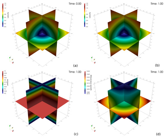
Figure 1.
Initial and final velocity (a,b), pressure (c), and total energy (d) for the vortical flow problem.
Table 2.
errors and convergence rates for the vortical flow problem. The convergence rates in the last line are computed from Equation (16) based on the errors from the 48 M and 6 M meshes.
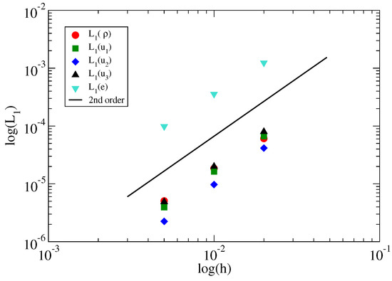
Figure 2.
errors of the density, velocity components, and internal energy in the vortical flow problem.
3.2. Validation
To demonstrate the solver in a 3D complex-geometry case, we computed the well-documented aerodynamic flow over the ONERA M6 wing, see, e.g., [12]. The available experimental data of the pressure distribution along the wing allow validation of the numerical method. The initial conditions prescribed a Mach number of 0.84 and the velocity with an angle of attack of . At the outer surface of the domain, characteristic far-field boundary conditions are applied, while along the wing surface, symmetry (free-slip) conditions are set.
Since we know that the solution of this problem does not depend on time, the most efficient ways to compute it are to use implicit time marching or local time stepping [5], of which we implemented the latter, allowing to take larger time steps for larger computational cells. Local time stepping is implemented by defining a separate timestep for each gridpoint v:
and advancing the solution in every point using its own time step size . The numerical solution is marched until a steady solution reached. The stopping criterion is determined by a sufficiently small value of the 2–norm of the density residual as
The computational mesh consists 710,971 tetrahedra and 131,068 points. The surface mesh is shown in Figure 3 together with the converged computed pressure contours on the upper and lower surfaces of the wing. Figure 4 shows how the density residual converges to steady state. The wall-clock time for this computation was about 2 min using 32 CPUs. The distribution of the computed pressure coefficient, , is compared to experimental data [13] at various semispans in Figure 5. Here, the ∞ subscript denotes the farfield conditions and u is the length of the velocity vector.
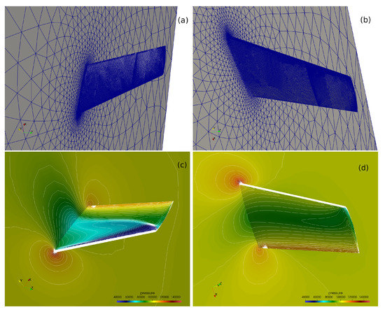
Figure 3.
Upper (a) and lower (b) sides of the surface mesh used for the ONERA M6 wing calculation. Computed pressure contours on the upper (c) and lower (d) surface.
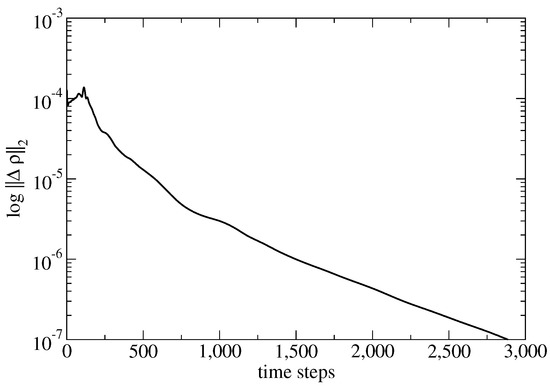
Figure 4.
Convergence history of the ONERA wing computation.
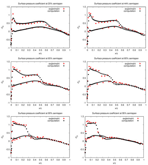
Figure 5.
Computed and experimental surface pressure coefficient at different semispans of the ONERA wing. Here, c denotes the length in of the wing cross section at the semispan location.
3.3. Automatic Load Balancing
With respect to solving partial differential equations on meshes, there is no magic using Charm++ compared to MPI: the computational domain is still decomposed and communication of partition-boundary data is still explicitly coded and communicated. However, an important difference compared to the usual divide-and-conquer strategy of domain decomposition is that Charm++ also allows combining this data-parallelism with task parallelism. As a result, various tasks (e.g., computation and communication) are performed independently, in arbitrary order, and are overlapped due to Charm++’s asynchronous-by-default paradigm. For an example of how task-parallelism can be specified in Charm++ with a different Euler solver, see [14].
Another unique feature of Charm++ compared to MPI is built-in automatic load-balancing. Charm++ can perform real-time CPU load measurement and, if necessary, can migrate data to under-loaded processors to homogenize computational load. This can be beneficial independent of its origin, i.e., adaptive mesh refinement, complex local equations of state, and CPU frequency scaling, or simply if some work units have a different number of boundary conditions to apply compared to others. Multiple load-balancing strategies are available in Charm++ and using them requires no extra programming effort: the feature is turned on by a command-line switch. Load balancing costs are negligible (compared to the physics operators) and can be beneficial for irregular work loads at any problem size, from laptop [15] to cluster [14].
We computed the Sedov problem [16], widely used in shock hydrodynamics, to test the ability of numerical methods to maintain spherical symmetry. In this problem, a source of energy is defined to produce a shock in a single computational cell at the origin at as:
In this smulation we use . These initial conditions correspond to pressure ratios of – across a single element at the origin and are specified so that the source of energy produces a shock location of at . Thus, the 1D solution in time is a spherically spreading wave starting from a single point. We used a 3D computational domain that is an octant of a sphere, with the mesh consisting of 23,191,232 tetrahedra and 3,956,135 points. The computed density is compared to the semi-analytic solution at in Figure 6.
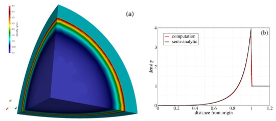
Figure 6.
Surface density (a) and its radial distribution (b) at from the Sedov calculation.
To exercise Charm++’s built-in load balancing, we modified the Sedov problem by adding extra computational load to the function that computes the pressure based on density and internal energy: if fluid density > 2.0 then sleep (1 ms). This increases the cost of the equation of state evaluation, whose location propagates in space and time, which induces load imbalance across multiple mesh partitions in parallel. Figure 7 and Table 3 show the effect of load balancing on wall-clock time: in this particular case, the extra load would make the simulation about more expensive. This is made faster using load balancing.
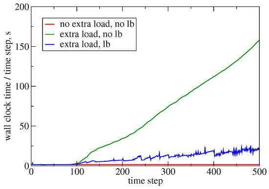
Figure 7.
Measured wall-clock time of each time step during the Sedov calculation without extra load, as well as with extra load with and without load balancing. The area below each curve is proportional to the total computational cost.
Table 3.
Timings for the Sedov problem with and without load balancing.
We emphasize that we wrote no load-balancing code: we simply ensure overdecomposition (in this case, we used 6399 mesh partitions on 32 CPUs) and turn on load balancing; the runtime system measures real-time CPU load and automatically performs object migration to homogenize the load. While this example was run on a single computer, experience shows that the benefits of such load balancing can be even greater on large distributed-memory machines [14].
4. Impact and Conclusions
We presented an open-source code, Xyst (https://xyst.cc, accessed on 27 March 2023), for the simulation of compressible flows. The software implementation with documentation, testing, code quality assessment, and reproducible examples is made publicly available. Xyst enables the use of advanced runtime system features not directly available for other flow solvers using MPI, which would often require advanced computer science expertise and significant ongoing nontrivial software maintenance effort in production. Xyst can be used to solve complex-geometry engineering problems involving 3D compressible flows at large scales. Building on the publicly available source code can also be used as a basis of multiphysics simulations.
Using Charm++ (http://charmplusplus.org, accessed on 27 March 2023) as its parallel programming paradigm, the implementation enables combining data-, and task-parallelism in an asynchronous-by-default execution model. Using a single software abstraction on both shared-, and distributed-memory machines enables performance and scalability. Automatic load balancing, built into Charm++, enables redistribution of heterogeneous computational load based on real-time CPU load measurement. The runtime system also features automatic checkpointing, fault tolerance, resilience against hardware failure, and supports power- and energy-aware computation without extra effort required from the application programmer.
Author Contributions
Conceptualization, A.P. and J.W.; Methodology, J.B., M.C. (Marc Charest), A.P. and J.W.; Software, J.B., M.C. (Marc Charest) and A.P.; Validation, J.B., M.C. (Marc Charest), P.R. and J.W.; Investigation, J.B.; Resources, M.C. (Mátyás Constans), Á.K., L.K., P.R. and J.W.; Data curation, J.W.; Project administration, J.B.; Funding acquisition, Z.H. All authors have read and agreed to the published version of the manuscript.
Funding
Co-funded by the European Union, this work has received funding from the European High Performance Computing Joint Undertaking (JU) and Poland, Germany, Spain, Hungary, and France under grant agreement number: 101093457. This work was also partially supported by the U.S. Department of Energy through the Los Alamos National Laboratory. Los Alamos National Laboratory is operated by Triad National Security, LLC, for the National Nuclear Security Administration of the U.S. Department of Energy (Contract No. 89233218CNA000001).
Data Availability Statement
The source code and data presented in this study are openly available at https://xyst.cc under “Examples”.
Acknowledgments
We thank Hong Luo and Weizhao Li of North Carolina State University for the fruitful discussions regarding local time stepping, the ONERA wing meshes and the experimental data.
Conflicts of Interest
The authors declare no conflict of interest.
References
- Luo, H.; Baum, J.D.; Löhner, R.; Cabello, J. Adaptive Edge-Based Finite Element Schemes for the Euler and Navier-Stokes Equations. In Proceedings of the 31st Aerospace Sciences Meeting, Reno, NV, USA, 1–14 January 1993. [Google Scholar]
- Luo, H.; Baum, J.D.; Löhner, R. Edge-based finite element scheme for the Euler equations. AIAA J. 1994, 32, 1183–1190. [Google Scholar] [CrossRef]
- Waltz, J. Derived data structure algorithms for unstructured finite element meshes. Int. J. Numer. Methods Eng. 2002, 54, 945–963. [Google Scholar] [CrossRef]
- Löhner, R.; Galle, M. Minimization of indirect addressing for edge-based field solvers. Commun. Numer. Methods Eng. 2002, 18, 335–343. [Google Scholar] [CrossRef]
- Löhner, R. Applied Computational Fluid Dynamics Techniques: An Introduction Based on Finite Element Methods; Wiley and Sons Ltd.: Chichester, UK, 2008. [Google Scholar]
- Acun, B.; Gupta, A.; Jain, N.; Langer, A.; Menon, H.; Mikida, E.; Ni, X.; Robson, M.; Sun, Y.; Totoni, E.; et al. Parallel Programming with Migratable Objects: Charm++ in Practice. In Proceedings of the International Conference for High Performance Computing, Networking, Storage and Analysis (SC ’14), New Orleans, LA, USA, 16–21 November 2014; pp. 647–658. [Google Scholar] [CrossRef]
- Waltz, J.; Morgan, N.; Canfield, T.; Charest, M.; Risinger, L.; Wohlbier, J. A three-dimensional finite element arbitrary Lagrangian-Eulerian method for shock hydrodynamics on unstructured grids. Comput. Fluids 2013, 92, 172–187. [Google Scholar] [CrossRef]
- Waltz, J. Microfluidics simulation using adaptive unstructured grids. Int. J. Numer. Methods Fluids 2004, 46, 939–960. [Google Scholar] [CrossRef]
- Davis, S.F. Simplified second-order Godunov-type methods. SIAM J. Sci. Stat. Comput. 1988, 9, 445–473. [Google Scholar] [CrossRef]
- Hirsch, C. Numerical Computation of Internal and External Flows: The Fundamentals of Computational Fluid Dynamics; Wiley and Sons: Chichester, UK; New York, NY, USA; Brisbane, Australia; Toronto, ON, Canada; Singapore, 2007. [Google Scholar]
- Waltz, J.; Canfield, T.; Morgan, N.; Risinger, L.; Wohlbier, J. Manufactured solutions for the three-dimensional Euler equations with relevance to Inertial Confinement Fusion. J. Comput. Phys. 2014, 267, 196–209. [Google Scholar] [CrossRef]
- Luo, H.; Baum, J.; Löhner, R. A Fast, Matrix-Free Implicit Method for Compressible Flows on Unstructured Grids. J. Comput. Phys. 1998, 146, 664–690. [Google Scholar] [CrossRef]
- Schmitt, V.; Charpin, F. Pressure Distributions on the ONERA-M6-Wing at Transonic Mach Numbers, Experimental Data Base for Computer Program Assessment; Report of the Fluid Dynamics Panel Working Group 04; Technical rep4ort, AGARD AR-138; 1979. Available online: https://www.sto.nato.int/publications/AGARD/AGARD-AR-138/AGARD-AR-138.pdf (accessed on 27 March 2023).
- Bakosi, J.; Bird, R.; Gonzalez, F.; Junghans, C.; Li, W.; Luo, H.; Pandare, A.; Waltz, J. Asynchronous distributed-memory task-parallel algorithm for compressible flows on unstructured 3D Eulerian grids. Adv. Eng. Softw. 2021, 160, 102962. [Google Scholar] [CrossRef]
- Li, W.; Luo, H.; Bakosi, J. A p-adaptive Discontinuous Galerkin Method for Compressible Flows using Charm++. In Proceedings of the AIAA Scitech 2020 Forum, Orlando, FL, USA, 6–10 January 2020. [Google Scholar]
- Sedov, L. Similarity and Dimensional Methods in Mechanics, 10th ed.; Elsevier: Amsterdam, The Netherlands, 1993. [Google Scholar] [CrossRef]


Disclaimer/Publisher’s Note: The statements, opinions and data contained in all publications are solely those of the individual author(s) and contributor(s) and not of MDPI and/or the editor(s). MDPI and/or the editor(s) disclaim responsibility for any injury to people or property resulting from any ideas, methods, instructions or products referred to in the content. |
© 2023 by the authors. Licensee MDPI, Basel, Switzerland. This article is an open access article distributed under the terms and conditions of the Creative Commons Attribution (CC BY) license (https://creativecommons.org/licenses/by/4.0/).