Abstract
Transition of ideal, homogeneous, incompressible, magnetohydrodynamic (MHD) turbulence to near-equilibrium from non-equilibrium initial conditions is examined through new long-time numerical simulations on a periodic grid. Here, we neglect dissipation because we are primarily concerned with behavior at the largest scale which has been shown to be essentially the same for ideal and real (forced and dissipative) MHD turbulence. A Fourier spectral transform method is used to numerically integrate the dynamical equations forward in time and results from six computer runs are presented with various combinations of imposed rotation and mean magnetic field. There are five separate cases of ideal, homogeneous, incompressible, MHD turbulence: Case I, with no rotation or mean field; Case II, where only rotation is imposed; Case III, which has only a mean magnetic field; Case IV, where rotation vector and mean magnetic field direction are aligned; and Case V, which has nonaligned rotation vector and mean field directions. Dynamic coefficients are predicted by statistical mechanics to be zero-mean random variables, but largest-scale coherent magnetic structures emerge in all cases during transition; this implies dynamo action is inherent in ideal MHD turbulence. These coherent structures are expected to occur in Cases I, II and IV, but not in Cases III and V; future studies will determine whether they persist.
1. Introduction
“One cannot deal with the physics of cosmic fluids without encountering at almost every turn the problem of turbulence.”[1]
In particular, one encounters the problem of magnetohydrodynamic (MHD) turbulence, since ‘cosmic fluids’, such as those found in planetary interiors and in stars, are electrically conducting and stirred into turbulence by buoyant forces. A universal feature of these objects is that they are rotating and often possess a quasi-stationary, mostly dipole magnetic field, i.e., a magnetic coherent structure. Just over a hundred years ago, ref. [2] hypothesized that internal magnetic fields coupled to fluid motions within the Sun, and by extension, the Earth, were responsible for the creation and maintenance of global magnetic dipole fields. Determining exactly how this was done came to be called ‘the dynamo problem’.
In regard to Earth, numerical simulations of the geodynamo [3,4,5] established that MHD processes within the Earth are capable of creating a magnetic field similar to the actual geomagnetic field, including reversals of the dominant dipole component. In addition, there have been many laboratory experiments [6], some of which have shown the growth of a self-generated magnetic field, i.e., a dynamo [7,8,9]. Although numerical simulations have been successful in proving the MHD nature of the geodynamo and experiments have shown a dynamo effect, the fundamental MHD origin of the dominant, quasi-steady geomagnetic dipole field still appear to be a theoretical mystery [10].
Our approach to resolving this mystery is to study three-dimensional (3-D) homogeneous, incompressible MHD turbulence, i.e., to examine a turbulent magnetofluid confined to a 3-D periodic box (a three-torus). This allows for the use of Fourier expansions to represent turbulent velocity and magnetic fields in order to study the nonlinear dynamics of a magnetofluid without the complicating factor of boundary conditions; in fact, introducing boundaries with no-slip conditions also requires introducing compressibility [11] and further complicates the problem. Fourier methods transform the problem from the partial differential equations of MHD (presented in Section 2.1) in -space (physical space) to a dynamical system of nonlinear, coupled ordinary differential equations in -space (Fourier space), which describe the evolution of the Fourier modes associated with velocity and magnetic field; this is discussed in Section 2.3. In -space, the continuum magnetofluid is represented on an grid of velocity and magnetic field values, while in -space, it is represented by the velocity and magnetic vector Fourier coefficients and , where the wavevectors define length-scales , , in the turbulent magnetofluid and explicitly separate the largest length-scale modes from all of the smaller length-scale modes. This is particularly useful as the largest length-scale modes are analogous to the magnetic dipole components in a planet or star.
Viscous and ohmic dissipation occur in a real magnetofluid but ‘cosmic fluids’ generally have very large Reynolds numbers so that one may remove dissipation from a model system and study ideal homogeneous MHD turbulence for the following reason. We neglect dissipation because we are primarily concerned with behavior of a turbulent magnetofluid at the largest scale; large-scale dynamics have been shown to be essentially the same for ideal and real (forced and dissipative) MHD turbulence [12,13]. The real MHD equations appear in (1) and (2) of Section 2.1 and become the ideal MHD equations when we set the viscosity and magnetic diffusivity equal to zero. There are differences between solutions of the real and ideal MHD equations as the highest derivative terms (the dissipative terms) in the real MHD equations methods are removed to produce the ideal MHD equations; the connection between real and ideal solutions is examined by singular perturbation theory, e.g., [14]. These differences are critical in real fluid and MHD flows since there may be thin regions, such as boundary layers, where the second-order dissipative terms become dominant, or in regions far from boundaries where there is a direct cascade of energy to the dissipation length-scale and where, again, dissipative terms are dominant. However, ideal results are often very useful. For example, in studying fluid turbulence, while it is usually necessary to retain the dissipative term in the Navier–Stokes equation because it determines the wavenumber spectrum in the medium-scale inertial and small-scale dissipative ranges, it is nevertheless possible to use ideal results to draw conclusions on the nature of real, helical fluid turbulence [15].
The fundamental difference between fluid and MHD turbulence is induced by the presence of a dynamic magnetic field, in that fluid turbulence only has a direct cascade to higher wavenumbers [16], while MHD turbulence has an inverse cascade as well as a direct one [17]. This difference between fluid and MHD turbulence, due to the MHD inverse cascade, can create an energetically dominant large-scale magnetic field, depending on the particular case of MHD turbulence under consideration; these cases are given in Table 1 and the various helicities listed there are defined by equations described in the next two paragraphs and discussed in more detail in Appendix A. Ideal MHD statistical theory Appendix B predicts that in Cases I and II of Table 1, the large-scale magnetic field is quasi-stationary and has energy that is essentially equal to magnetic helicity, a result that also seems to apply to Case IV. These ideal MHD spectra are strongly peaked at the largest length scale, i.e., smallest wavenumber, where dissipation is weakest in the real case. That this survives the addition of forcing and dissipation to the magnetofluid has been shown in studies of helically forced, dissipative MHD turbulence using Fourier method simulations [12,13]. Thus, if we wish to study the large-scale dynamics and structure of MHD turbulence, either ideal or real MHD turbulence simulations can be employed. Here, we choose ideal MHD.

Table 1.
Cases and associated Runs with different integral invariants for ideal MHD turbulence. The ‘parallel helicity’ of Case IV is and occurs when , i.e., is parallel to .
Ideal MHD turbulence, as represented by a finite set of Fourier modes, is a conservative system with energy and up to two different helicities being integral invariants; again, the different cases are shown in Table 1. The number and form of the helical invariants depend on whether or not rotation or a mean magnetic field or both are imposed on the system (a mean magnetic field is one that is spatially and temporally constant and frame rotation is given by a vector ). Energy E, cross helicity , magnetic helicity and parallel helicity , as well as other quantities, are fully defined in Appendix A; here, we will, for easy reference and to serve as a ‘nomenclature section’, briefly discuss how E, , and , as well as other integrals, are determined.
First, we define the volume average of a quantity multiplied by a quantity as , which is an integral over the volume of interest, here, a periodic box of side length :
The -space functions and are Fourier transforms of the -functions and (Fourier transforms are defined in Section 2.2). Energy and the various helicities listed in Table 1 are then ( is defined in terms of the magnetic vector potential , where , )
Again, velocity and magnetic fields can be represented in -space or -space; their basic equations are given in (1) and (2) for -space and (23) and (24) for -space, and either set can be used to prove invariance. In terms of the mean magnetic field and rotation vector magnitudes and , one defines the ratio when is parallel to . Other quadratic forms, in addition to those given above, are also useful measures of the turbulent state:
Above, we have (magnetic energy), (kinetic energy), (kinetic helicity, where is the vorticity), A (mean squared vector potential), (‘enstrophy’, i.e., mean squared vorticity) and J (mean squared electric current, where ); please note that enstrophy is different from rotation vector magnitude . For the computer runs discussed here, time-averages of these appear in Table 2.
Table 2.
Time averages and standard deviations (avg ± std) for various global quantities over the last half of each run are given below for six new ideal MHD turbulence long-time runs A, B, C, D, E and F. These global quantities are: energy E, kinetic energy , magnetic energy , mean squared vector potential A, kinetic helicity , magnetic helicity , cross helicity , parallel helicity , enstrophy and mean squared current J.
The ideal invariants given in Table 1 can be used to create a multi-invariant canonical probability density function and a statistical mechanics applicable to ideal MHD turbulence (Appendix B). This statistical theory was initiated by [18], applied to fluid turbulence by [16] and to MHD turbulence by [17,19]; these initial results were extended later, e.g., [20,21,22,23,24]. This extension is relevant to the planets and stars as it provides an, at least qualitative, explanation for the emergence of a dominant, quasi-stationary, dipole magnetic field through broken ergodicity, which is defined by [25] as occurring if ‘In a system that is non-ergodic on physical timescales the phase point is effectively confined in one subregion or component of phase space’. The phase space itself is defined by the real and imaginary parts of the coefficients of the independent Fourier modes in the model system.
Numerical simulations have played an essential part in MHD turbulence research, starting with [26] using a grid (which was large for that time), while advances in computer hardware have allowed more recent simulations to have much larger grid sizes, e.g., [27]. However, these simulations were only run for short simulation times, with in the former and in the latter, as the emphasis was on large grid sizes rather than on longer simulation time. In contrast, we have focused on long-time runs with ∼10 to gather statistics and this dictated smaller grid sizes of [22,23,24]; there is always this trade-off between grid size and simulation time. To illustrate the trade-off between grid size and maximum simulated time, ref. [28] presented runs from up to , but as the grid size went up, the time-step size decreased and number of time-steps increased, so that simulation time (number of ‘eddy turnover times’) decreased and only for the run was quasi-equilibrium attained (see their figure 5).
Improved computational resources have allowed us to increase our grid size to while still keeping . We have recently run six of these simulations, each for over a million time-steps, in a reasonable amount of calendar time (over half a year each) and they allow us to examine the transition of ideal MHD turbulence for each of the cases in Table 1, where the runs associated with each case are indicated. All of our runs have moved through or are near the end of their transition periods and appear either to achieve equilibrium or to approach it asymptotically. Here, we focus on this initial period of transition to near-equilibrium and plan to examine the full equilibrium phase and present results in the future when these become available.
From our earliest numerical simulations [20] to those presented here, we have consistently seen the lowest-wavenumber (largest length-scale) modes grow from very small initial values into energetic, quasi-stationary, coherent structures. To understand this, it is necessary to develop the statistical theory of ideal MHD turbulence beyond that introduced by [17]. In particular, we analyzed the entropy of the model dynamical system to discover the origin of this energetic structure; we have presented this analysis before [24,29] and will place it here in Appendix B. Furthermore, the statistical mechanics of an ideal, turbulent magnetofluid in a periodic box is essentially the same as that of one contained in a spherical shell [30] and thus, the smallest wavenumber Fourier modes are surrogates for geomagnetic dipole components.
Key discoveries in our past work are: (i) That the energy of a quasi-stationary magnetic dipole in Cases I and II is directly proportional to the absolute value of the magnetic helicity of the equilibrium turbulent magnetofluid [29,31]; this also appears to apply to Case IV, as will be shown here; and (ii) that the assumed ergodicity of the statistical ensemble is actually broken at the largest scale [20,24]. Again, these ideal results have been seen to apply at the largest length-scale to real (i.e., forced and dissipative) MHD turbulence [12,13]; thus, modeling and theory provide a solution to the ‘dynamo problem,’ at least for the model systems considered here. (Again, ideal MHD statistical theory is reviewed in Appendix B of this paper for ease of referral).
Next, following a brief discussion of the mathematical model and numerical procedure, new computational results drawn from simulations are presented. These are followed by a discussion of these results and their relevance to the dynamo problem. Lastly, we offer a conclusion to summarize our results and emphasize their importance.
2. Mathematical Model
2.1. Basic Equations
Magnetohydrodynamics (MHD) is the physics of electrically conducting fluids and principles and applications can be found in, e.g., [32,33], as well as in many other texts. The nondimensional form of the 3-D incompressible MHD equations in a rotating frame of reference with constant angular velocity and mean magnetic field (i.e., constant in space and time) can be written as
These are described, for example, by [22]; these equations can be augmented to include thermal effects in the Boussinesq approximation [34], but we will not consider this here. Above, and are the turbulent velocity and magnetic fields, respectively. Velocity and magnetic fields are solenoidal: , as is appropriate for laboratory experiments and the Earth’s outer core [3]. The vorticity and electric current density are defined by
Nondimensional density does not appear in (1) because it equals unity. The symbols in (1) and in (2) are shorthand for and , i.e., the inverses of the kinetic and magnetic Reynolds numbers, respectively. In the dimensional form of the equations, is the kinematic viscosity, while is the magnetic diffusivity and for ideal MHD turbulence. Again, we avoid the complication of boundary conditions by placing the magnetofluid in a periodic box and expanding the various fields in terms of Fourier series.
In studying MHD turbulence, it is also possible to use other orthogonal function expansions, such as those appropriate to a cylinder [35], sphere [36] or spherical shell [30]. However, the statistical mechanics of ideal MHD turbulence has the same form and predictions as in the Fourier case. In addition, the Fourier spectral transform methods used to simulate MHD turbulence in a periodic box are much more computationally efficacious in that they allow for larger grid sizes (more dynamical resolution) and longer runs (for time averaging). In fact, no spectral transform methods for these other geometries yet exist (the creation of which may be considered a ‘grand computational challenge’) and nontransform methods [36,37], in comparison, will always have insufficient resolution. In essence, Fourier transform methods in a periodic box are efficient and also serve as a surrogate for methods based on other orthogonal function expansions more suited to other geometries.
2.2. Fourier Representation
Discrete Fourier transforms for and , connecting -space to -space, are
Here, N is the number of grid points in each -space dimension, so we have a grid of points. The set of positions and wave vectors (modes) appearing in (4) and (5) are
The components and , , are integers. The satisfy , while the integers lie in the range and ; thus, there are points in both spaces. The dot product in (4) and (5) is
The Fourier coefficients and are nonzero only for , where . The exact value of K is set by a de-aliasing requirement of [38]: is the largest integer such that , e.g., for , .
Note that the reality of and imply that and . In a Cartesian coordinate system, and are
The vector fields and can be defined in a similar manner.
The periodic box of the model system is a cube of equal length edges. Although we will not do so here, we could have allowed for the possibility that it might be elongated or compressed in the x, y or z directions, which simulates a difference in oblateness that may occur in the Earth’s inner and outer cores. We ignore this possibility because we have examined it and the dynamical effect is insignificant when compared to rotation [29].
Dynamically interacting coefficients fit within a sphere of radius K in -space; all coefficients outside this -sphere, as well as at , are initially zero and remain so during any numerical simulation. Since and , only half of the that satisfy identify independent coefficients. Therefore, the number of independent modes is ; for example, with and , we have 459,950, while the actual numerical count is = 459,916.
In -space, the requirements become . Thus, and have two independent complex vector coefficients each, which can be defined as follows: First, determine a coordinate system for each by starting with a unit vector ; then choosing a unit vector orthogonal to , and then the remaining unit vector is a vector product of the first two, forming a right-handed orthonormal basis for each :
(This is similar to a Craya–Herring decomposition [39]). Explicit choices [23] for any of the will be mentioned as needed.
In terms of the defined above, the Fourier vector coefficients (9) and (10) are
However, an equivalent but very useful helical representation is:
Here, the positive and negative helicity unit vectors and components are
Note that . The orthonormality properties of the are
An important property of the helical unit vectors concerns the curl operation:
The vorticity and current in helical form are then
Thus, the helical ± components of vorticity and current are directly connected to velocity and magnetic field ± helical components. The helical representation is very useful for theoretical analysis and graphical presentation of numerical data, although numerical simulation is actually performed using the Cartesian components (9) and (10).
2.3. A Dynamical System
The Fourier-transformed 3-D MHD equations are found by placing expansions for and of the form (4) into (1) and (2). The result is a set of coupled, nonlinear ordinary differential equations that represents a dynamical system in the sense of [40]:
The nonlinear terms denoted by are vector convolutions:
The double summation in (25) is over all wavevectors and inside the truncation volume in -space that satisfy . In 3-D numerical simulations, these equations are integrated as described in Section 3. For , the phase space of the dynamical system (23) and (24) has a dimension of = 3,679,328, as discussed in Appendix B. For ideal MHD, Table 1 indicates that the dynamical system conserves energy and various helicities depending on whether and are zero or not; these quantities and others are defined in Appendix A. The important Case II of Table 1, where and , applies to the Earth and most other planets (and stars), so in these cases, energy and magnetic helicity are of primary interest. The Cases III, IV and V, where , are appropriate for laboratory experiments and perhaps compact regions of solar wind turbulence where is the local interplanetary magnetic field.
2.4. Linear Modes
Using (11)–(18), the MHD Equations (23) and (24) can be linearized to yield
These can be put into a matrix form:
It is a straightforward procedure to find linear eigenmodes of (28) by diagonalizing ; there is one transform matrix for each :
The solution to (28) are the eigenmodes
where the time dependence of the linear modes is in the matrix
In the linear case, is constant, while in the nonlinear case, it becomes time-dependent. In slightly more detail, has the form
The matrix elements , , are given in (30).
If there is no nonlinearity, and of (34) will have constant, complex values determined by the initial conditions; they are the coefficients of traveling helical waves∼ if the are nonzero. If there is nonlinearity, then these coefficients will generally change with time and it is these changes that contain information about MHD turbulence.
3. Numerical Procedure
A Fourier spectral transform method [41] on an grid with is used; the minimum wave number is and the maximum wave number is . Time-integration is performed with a third-order Adams–Bashforth-Adams–Moulton method [42] with a time-step of ; initial, non-equilibrium magnetic and kinetic modal energy values (spectra) are ∼∼, where . Viscosity and magnetic diffusivity are set to zero so that the flow is ideal. A grid size of was used so that the six single core Runs listed in Table 1 could be completed in a reasonable amount of time with the resources available, the Hopper Cluster at George Mason University, with each simulation running at ≈11 ; thus, a single run of requires about 36 weeks of CPU time.
As mentioned, six computer simulations covering the five cases in Table 1 have been run and are identified in that table. The ideal invariants for each case are quadratic forms (global quantities) with terms that are scalar products of the vector Fourier coefficients and , with , as defined in Appendix A. The partial differential equations for MHD in -space are given by (1) and (2), while the transformed set of ordinary differential equations in -space are given by (23) and (24). The set of equations in -space is a finite dynamical system, as discussed in Section 2.3. The -space Equations (23) and (24) are numerically integrated to advance the and , as described in Section 3.
As seen in Table 1, the integral invariants of ideal MHD turbulence are the volume-averaged energy E and magnetic helicity when , as well as the cross helicity when and when . In a numerical simulation, these ideal invariants typically have a standard deviation of less than 1% per million time-steps, while kinetic helicity , though an ideal invariant for hydrodynamic turbulence, falls to zero very quickly and then has small fluctuations about that value, as Table 2 shows. We mentioned that these runs came to ‘near equilibrium’. To understand what this means, consider Figure 1 where we show, at different times for Runs 1 and 4, the average magnetic and kinetic energy spectra, and , for modes with the same value of . There are 3036 different values of , where , for ; the number of independent (i.e., but not ) is .
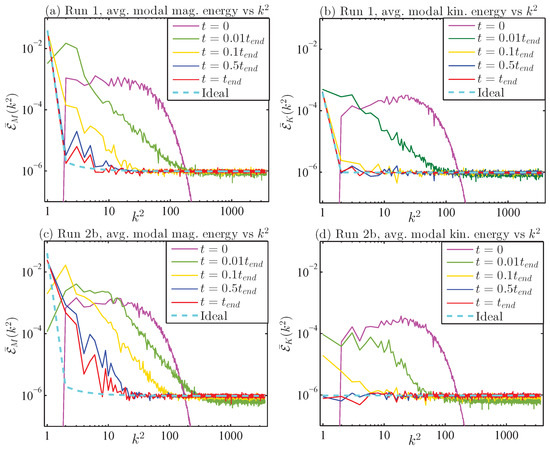
Figure 1.
Average magnetic and kinetic energy spectra, and , for Runs 1 and 2b. These are averages over modes with the same value of ; there are 3036 different values of , where , for . The spectra are shown for times , , and , where for Run 1 and 1037 for Run2b. Spectra are approaching their expectation values and are near equilibrium; they are in true equilibrium when they fully match the ideal expectation values.
The definitions of the averaged spectra and are
Here, is the number of independent that satisfy . The number jumps around as increases; for example,
(We have whenever ; see [43]). The full energy spectra are at each value of and thus jumps wildly as increases, which is why we prefer to look at the average energy spectra (35) and (36), as in Figure 1. (However, its running average over near neighbors is well approximated by .)
If we use the results in Appendix C or in [24], we find that the ideal expectation values of and are
Here, and , and are the normalized inverse temperatures related to inverse temperatures appearing in the phase space probability density (A20); please see Appendix B for details. For each of the cases, , and are determined by numerically finding the minimum of the entropy functional (A38) with the proviso that for Case II (Runs 2a and 2b), ; for Case III (Run 3), ; and for Case V (Run 5), . The values of , and for the different runs are given in Table 3.
Table 3.
Values of the inverse temperatures , and for the Runs in Table 1 with the proviso that for Runs 2a and 2b, ; for Run 3, ; and for Run 5, and . When needed, , , and took their values from , and , respectively, in Table 2. (The need for precision here is due to the possible smallness of the denominators in (38) and (39)).
The spectra are shown in Figure 1 for times , , , and , where for Run 1 and 1037 for Run2b. The spectra are approaching their expectation values and are near equilibrium; when they fully match the ideal expectation values, then they are in true equilibrium. The spectra and for Runs 3 and 5 will both be similar to those in Figure 1d, i.e., becoming flat, while the spectra for Run 4 will be similar to Figure 1a,b, though not as highly peaked at .
4. Computational Results
In Figure 2 and Figure 3, we show how the six runs in Table 1 change over time with respect to volume-averaged energy E, magnetic energy , kinetic helicity , mean squared magnetic vector potential A, cross helicity , magnetic helicity , enstrophy (mean squared vorticity) and mean squared electric current J; for Run 4, parallel helicity is also shown; again, please see Appendix A for precise definitions of these quantities. The time-averages and standard deviations for these quantities over the course of the runs are given in Table 2. For each run in Table 2, the quantities that are supposed to be conserved are, in fact, conserved as shown in Figure 2 and Figure 3. The most conserved quantity, by far, is the magnetic helicity in Runs 1, 2a and 2b. Those quantities in Table 2 that have standard deviations larger in magnitude than their average values are basically just fluctuating around zero; in particular, this seems to be true for the kinetic helicity in every run except for Run 4. Note also that statistics for the enstrophy and mean squared current J are essentially equal in each run, indicating that smaller length-scales have equipartition in magnetic and kinetic energy.
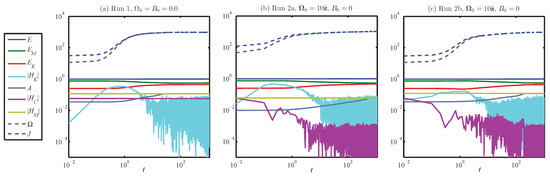
Figure 2.
Global quantities (see Appendix A) versus time t for homogeneous MHD Runs (a) 1, (b) 2a and (c) 2b. Notice how the integral invariants in Table 1 remain constant in their associated runs.
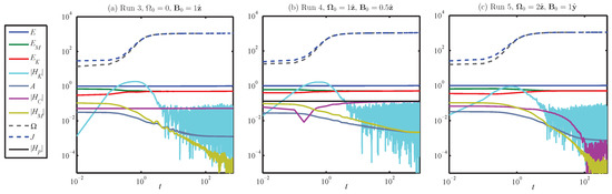
Figure 3.
Global quantities (see Appendix A) versus time t for homogeneous MHD Runs (a) 3, (b) 4 and (c) 5. Notice how the integral invariants in Table 1 remain constant in their associated runs.
For all the runs in Table 1, the values of all the and with were saved every 0.1 units of simulation time t (i.e., every 200 . From these, we can calculate a time history of modal energies
In Figure 4 and Figure 5, we see how the , , for each run varies with time. In Figure 4, and are compared to in each of Runs 1, 2a, 2b and 4; the result is compelling: is tending to become equivalent to , even for Run 4 where is not an integral invariant of the dynamical equations (instead, we use its value at for Run 4). This is again verification of the theoretical result given by [29,31], which also seems to apply to Run 4 because has reached a steady constant value. Figure 5 shows the evolution of for Runs 3 and 5; in these runs, ∼0, as Table 2 shows. Furthermore, in Figure 5a (Case III) and Figure 5b (CaseV), we see for aligned with ; additionally, in Figure 5b, is largest for aligned with , a ‘dipole alignment’ that has been seen before [29]. The ensemble prediction for both (a) and (b) in Figure 5 is , which is to be equally divided among the three ; thus, the steady values during transition here are several orders of magnitude too large, perhaps being supported by an increased magnetic energy inverse cascade during transition (and they do not correlate with ). Continuing these runs well into equilibrium (to be done) will determine whether these anomalous values persist.
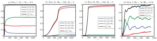
Figure 4.
Magnetic energies for the modes, normalized by , versus time t for Runs (a) 1, (b) 2a, (c) 2b and (d) 4. Notice how the total magnetic energy for , with time. (In (d), for Run 4 from Table 2 is used.)
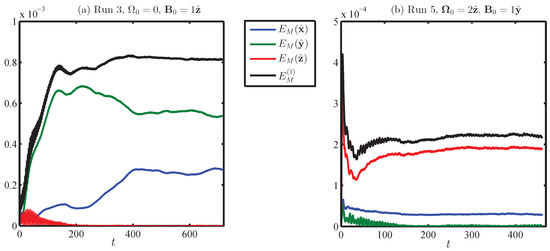
Figure 5.
Magnetic energies for the modes versus time t for Runs (a) 3 and (b) 5. In these runs, so that is not an invariant, although is an invariant in Run 4 where . In Run 5, is not aligned with , and the only invariant is E. The ensemble prediction for both (a,b) is , so the relatively very large and steady values during transition are anomalous.
In all six runs, a running time-average of the vector coefficients and was kept: and . The expectation has been that these will tend to zero; however, this is not the case for . These time-averaged vector coefficients can be used to calculate the ‘coherent total energy’ , ‘coherent magnetic energy’ and ‘coherent kinetic energy’ . The coherent kinetic and magnetic energies for the six runs are shown in Figure 6; the coherent kinetic energy levels off to a constant nonzero only for Run 1, as seen in Figure 6a, while the coherent magnetic energy levels off to a constant nonzero for Runs 1, 2a, 2b and 4, as seen in Figure 6b and these values of appear to approach their respective values of , which are shown in Figure 6c. With regard to Runs 3 and 5, Figure 6a,b indicates what seems to be exponential fall-off, while Figure 6c shows that for Runs 3 and 5 is fluctuating about zero; thus, the anomalously high values of for Runs 3 and 5 seen in Figure 5 may only be transitory.
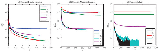
Figure 6.
Coherent (a) kinetic and (b) magnetic energies compared to (c) total magnetic helicity versus time t for all runs. In (a), a constant coherent has only appeared in Run 1, while in (b) Runs 1, 2a, 2b and 4, constant coherent have evolved and in (c)—constant , with , as indicated in Figure 4.
After numerical integration, components of the vectors and can be transformed into helical components , , and , as discussed in Section 2.2. These are useful but can be further transformed into cyclic linear modes whose noncyclic factors are , , and , as defined in Section 2.4. If there were no nonlinear interactions in the MHD equations, the would be complex constants; however, the MHD equations are nonlinear, so the may wander around with time. Since we have recorded data that can give us the time-histories of these for , we can plot their trajectories on a complex plane and clearly see the nature of ideal MHD turbulence, at least at the larger length-scales (i.e., smaller wave numbers k). These ‘phase portraits’ are projections of the dynamical trajectory in the high-dimensional phase space onto a 2-D plane which enables us to visualize the concepts of coherent structure, broken ergodicity and broken symmetry (please see Appendix E for a review of these concepts). For the six runs discussed here, some phase portraits are shown in Figure 7, Figure 8, Figure 9, Figure 10, Figure 11, Figure 12 and Figure 13.
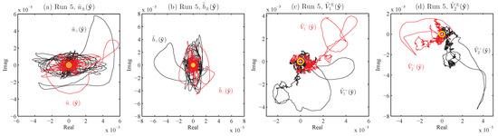
Figure 7.
Phase portraits from Run 5; white + marks the origin; variables are normalized by , . Yellow circles indicate predicted average magnitude. ∼ and ∼. Please see Section 2.4 for detailed discussions of relations between variables.
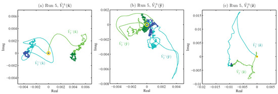
Figure 8.
Phase portraits of , (a) , (b) and (c) , from Run 5. (The variables are normalized by , .) Here, , and . Light parts are the full trajectories, while dark parts are the last half of the trajectories, i.e., from to . (a,c) indicate stationarity and coherent structure, dynamic results quite different from expected behavior as exemplified by (b). Yellow circles indicate the predicted average magnitude.
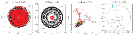
Figure 9.
Phase portraits from Run 4; the white + marks the origin; the variables are normalized by , . Parts (a,b) show phase trajectories of and before cyclic behaviors is removed. In (c) is an example of trajectories when cyclicity is removed. In (d), stationarity indicates coherent structure. The yellow circle in (c) indicates predicted average magnitude of each variable; the large black circle in (d) has radius , where Run 4 is from Table 2. Here, , , and .
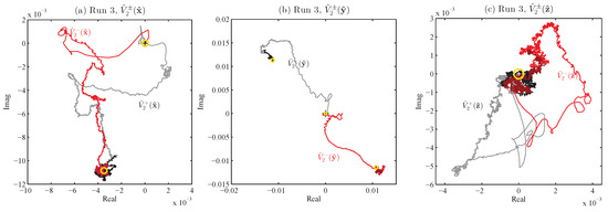
Figure 10.
Phase portraits from Run 3; + marks the origin; the variables are normalized by , . The yellow circles around the origin are the expected average magnitudes; in (a–c), these circles have also been placed around the ends of the trajectories, indicating that the fluctuation levels are as predicted, but the mean values are far from zero. Here, , and ∼.
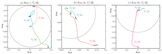
Figure 11.
Phase portraits from Runs (a) 1, (b) 2a and (c) 2b; + marks the origin; the variables are normalized by , . Light parts are the full trajectory, while dark ends are from the last half of the trajectory, i.e., from to . The black circles have radius . Please see Figure 12 for close-ups of ends of trajectories in (a). In these figures, .
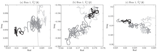
Figure 12.
Close-up phase portraits of , (a) , (b) and (c) , from Run 1; these are the ends of the trajectories shown in Figure 11. (The variables are normalized by , .) Light gray is part of the full trajectory, while dark gray is the last half of the trajectory, i.e., from to , and the black part is from to . In these figures, .
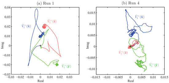
Figure 13.
Phase portraits of , , and , for (a) Run 1 and (b) Run 4. These are the only variables exhibiting coherent structure. (The variables are normalized by , ). Here, , except in (b), where ∼.
Phase portraits from Run 5 are presented in Figure 7. Referring to Section 2.4, we see that (with and )
The transformed variables have no cyclic time variation and their evolution from initial values (which are all close to zero) shows the effect of the nonlinear terms in (23) and (24). In Figure 7, the appear to be zero-mean random variables whose fluctuations match statistical expectations as to mean and standard deviation; in fact, all for Case V of Table 1 are expected to be zero-mean random variables with the same standard deviation. (Please see Appendix B of a review of the statistical theory.)
However, if we take a look at Figure 8 corresponding to Run 5, we see the unexpected nonlinear behavior of (a) and (c) ; we compare this with the trajectory of that is shown in Figure 8b (which is the same as Figure 7c). In other words, what we see in Figure 8a,c are not the expected zero-mean random variables of small fluctuation, but very large nonzero mean random variables of small fluctuation; we see ‘broken ergodicity’ (as discussed in Appendix E). The quasi-steady end stage of the trajectories of Figure 8a,c represent a quasi-stationary coherent structure in the magnetofluid. This is, at first, surprising, but nonetheless, it occurs: ergodicity is dynamically broken for Case V, at least during transition to equilibrium; however, longer run-times (which are planned) are needed to examine behavior in equilibrium. At the largest length-scales, where , these coherent structures seem very robust during transition in Run 5 and in other runs where they appear, while at smaller length-scales, , ‘random walk’ trajectories appear to be converging towards zero-mean, both for Run 5 and for the other Runs in Table 1; again, longer run-times are planned to study equilibrium behavior.
Phase portraits from Run 4 are shown in Figure 9. Parts (a) and (b) show phase trajectories of and before cyclic behavior is removed. In Figure 9c, an example is given of trajectories where cyclicity is removed. In Figure 9d, quasi-stationarity indicates coherent structure. Again, statistical expectations are that all Case IV variables have zero-mean; yet, they do not behave as expected and indicate that broken ergodicity has occurred. In fact, the behavior seen in Figure 9d is the same as that expected of Case II in Table 1, i.e., the three magnetic modes altogether have energy and thus, average magnitudes each of . (In Figure 9d, from Table 2 is used for .) In Figure 9, these Run 4 are, explicitly (with and ),
In Figure 9d, we also see ‘broken symmetry’ in that the magnitudes of the quasi-stationary values of , and are unequal.
Phase portraits from Run 3 are shown in Figure 10. The yellow circles around the origin show the expected average magnitudes; in (a) and (b), these circles have also been placed around the ends of the trajectories, indicating that the fluctuation levels are as predicted, but the values are far from the predicted zero-mean, compared with the expected behavior seen in Figure 10c. In Figure 10, the are [with ], explicitly
The statistical ensemble expectation is that the for all , , in addition to being zero-mean, will have the same standard deviation, . In Figure 10a,b, we see that this expectation is not met and that, again, we have broken ergodicity manifested during transition as large-scale coherent structure. Additionally, the magnitudes at the ends of the trajectories in Figure 10a,b are much larger than predicted; whether or not these persist will be determined by allowing Run 3 to continue running, as is planned for the next phase of our work.
Phase portraits from Runs (a) 1, (b) 2a and (c) 2b are presented in Figure 11. Light parts are the full trajectory, while dark ends are from the last half of the trajectory, i.e., from to . The black circles have radius , where , is given for Runs 1, 2a and 2b in Table 2. In Figure 11, all . These phase trajectories all clearly show broken ergodicity and broken symmetry, for although their rms magnitudes are predicted, their quasi-stationarity is not and is, instead, a dynamical phenomenon. Now, we turn to Figure 12 for close-ups of ends of Run 1 trajectories in Figure 11a; these also serve as examples of the level of quasi-stationarity in Runs 2a and 2b.
In Figure 12, we see close-up phase portraits of , (a) , (b) and (c) , from the ends of the Run 1 phase trajectories shown in Figure 11a. Light gray is part of the full trajectory, while dark gray is the last half of the trajectory, i.e., from to , and the black part is from to . Again, in these figures, . The small extent of the parts from to indicate the high level of quasi-stationarity in the coherent structure that has been created as MHD turbulence transitioned from an initially small-scale distribution of energy at to the states appearing in Figure 11; in this figure, Runs 2a and 2b are particularly relevant to understanding the origin of the MHD dynamo in rotating planets and stars: it is an inherent property of MHD turbulence. Again, Figure 12 presents a close-up example of the energetic, quasi-stationary, coherent structures that arise in MHD turbulence.
The energetic coherent structure generated by MHD turbulence is essentially magnetic. However, some coherent structure is exhibited by the velocity field, specifically in Runs 1 and 4. In Figure 13, you will find phase portraits of , where , and , for (a) Run 1 and (b) Run 4. These runs are the only ones with variables (these are inertial waves) exhibiting coherent structure. These are all purely helical velocity variables , except in (b), where the one Run 4 variable exhibiting coherence is mostly kinetic but with a small part that is magnetic:
Once again, details of the variables and their relation to the primary variables and can be found in Section 2.4.
5. Discussion
The primary discovery here is that all of the five Cases of ideal MHD turbulence in Table 1 make a transition from small-scale initial conditions into a near-equilibrium state that contains coherent structure. Since the ensemble prediction is that all variables have zero-mean, what we have is broken ergodicity (and broken symmetry; please see Appendix E). The most surprising phenomena are that Run 3 (Case III) and Run 5 (Case V) developed coherent structure during transition. This was not expected, although coherent structure was expected in Run 1 (Case I), as well as Runs 2a and 2b (both Case II), since similar coherent structure has been seen in numerical simulations of both ideal [24,44] and real [12,13] MHD turbulence.
Coherent structure is identified by quasi-stationary , as Figure 2, Figure 3, Figure 4, Figure 5, Figure 6, Figure 7, Figure 8, Figure 9, Figure 10, Figure 11, Figure 12 and Figure 13 show. This discovery was facilitated through Fourier spectral method numerical simulations on a grid. It has been shown with similar simulations that coherent structure also appears in dissipative MHD turbulence forced at an intermediate wavenumber and that these dissipative, forced results obey ideal MHD statistical theory at the largest wave lengths [12,13]. Furthermore, the statistical theory of ideal MHD turbulence developed for a periodic box has the same form as that developed for a spherical shell [30]. Therein lies the importance of ideal results to the real MHD turbulence contained in planetary liquid cores and in the convective layers of stars: it is a basic, qualitative explanation of how astrophysical dipole magnetic fields arise and thus, a solution to ‘the dynamo problem’.
MHD turbulence in astrophysical objects is covered by Cases I and II in Table 1 and as has been shown here with simulations, these are the cases with the most energetic coherent structure, i.e., quasi-stationary ‘dipole magnetic fields.’ The energy in the large-scale magnetic field is directly proportional to the total magnetic helicity in the turbulent magnetofluid; in the ideal case, this is set by initial conditions, while in the real case, the dipole field grows through inverse cascade and dynamic alignment as long as whatever forcing mechanism is present injects magnetic helicity of primarily one sign into the magnetofluid [12,13]. The exact nature of the helical forcing is hidden from view deep within an astrophysical object, but our results imply that it must be there.
Cases III, IV and V of Table 1 all contain an external magnetic field and are thus related to terrestrial experiments with turbulent magnetofluids, e.g., tokamaks, or perhaps to concentrated regions of plasma within stellar winds, for example, rather than whole planets and stars. The statistical mechanics of ideal MHD turbulence (see Appendix B) tells us that the modal energies of Cases III and V are expected to be equipartitioned, while Case IV is expected to have much more energy in the modes. Thus, the coherent structure seen in Runs 3 and 5 is a surprise, while in Run 4, the surprise is that it appears to be like Case I or II once reaches an essentially constant value.
6. Conclusions
In summary, the primary discovery here is that all of the five Cases of ideal MHD turbulence in Table 1 have developed quasi-stationary coherent structure. These coherent structures appear robust as the runs appear to have finished or are close to finishing transition from initial conditions to an equilibrium state. However, the appearance of coherent structure for Cases III and V during transition to equilibrium may be transitory and further long-term computation is needed to examine these cases once they fully reach equilibrium. The importance of the computational and theoretical results, particularly for Cases I and II which are most relevant for planets and stars, is that they show that MHD turbulence, per se, is a dynamo. We intend to continue these runs beyond the values of given in Table 2 in order to examine MHD turbulence while in full, long-term equilibrium; we will report on the results when we have them.
Another direction future investigations can take is to add dissipation and forcing to our simulations as was done on grids [12,13]. The methods employed to force a model magnetofluid at intermediate wavenumbers are speculative because physical forcing mechanisms are hidden from observation within a planet or star. Nevertheless, having used a variety of mid-wavenumber, helical forcing methods on grids, we have always seen behavior analogous to ideal MHD turbulence at the smallest wavenumber, which is the emergence of large-scale coherent magnetic structure whose energy is determined by the amount of magnetic helicity in the magnetofluid turbulence. We would expect to see this in simulations, along with perhaps some novel effects, but this remains to be done.
The methods used here, numerical simulation and statistical analysis, may also profitably be used in examining other dynamical systems that have associated integral invariants. One example is a model of quantum electrodynamic turbulence [45] in which the coupled Dirac and Maxwell equations were numerically solved in a manner similar to that used here for a magnetofluid. This work was based on classical field theory but allowed for a nonperturbative approach. Another possible application is to study geometrodynamic turbulence, i.e., the evolution of space-time from arbitrary initial conditions; a preliminary numerical simulation could be based on the Einstein equations in a synchronous reference frame [46] before moving on to more general reference frames. These seem to be ‘grand challenge problems’ but should yield interesting results in terms of mathematics with perhaps some compelling physical relevance.
Funding
This research received no external funding.
Data Availability Statement
Data is available by contacting author.
Conflicts of Interest
The author declares no conflict of interest.
Appendix A. Global Quantities
Table A1.
Integral invariants for ideal MHD turbulence. The ‘parallel helicity’ of Case IV is and occurs when , i.e., is parallel to .
Table A1.
Integral invariants for ideal MHD turbulence. The ‘parallel helicity’ of Case IV is and occurs when , i.e., is parallel to .
| Case | Mean Field | Rotation | Invariants |
|---|---|---|---|
| I | E, , | ||
| II | E, | ||
| III | E, | ||
| IV | E, | ||
| V | E |
There are various important global quantities that can be expressed as averages over either -space or, equivalently, -space. We define the volume average of a quantity multiplied by a quantity as , which is an integral over the periodic box of side length :
and are Fourier transforms of and in the manner of (4) and (5).
Using (A1), the volume-averaged energy E, enstrophy , mean-squared current J, cross helicity , magnetic helicity and mean-squared vector potential A (the last two defined in terms of the magnetic vector potential , where , ) are
Since all functions are periodic in -space, we can use Equations (1) and (2), along with integration by parts to derive the following relations [22]:
When and , the quantities E, and are the traditional ideal integral invariants of MHD turbulence [1,18,47]. If , then (A5) indicates that is no longer an ideal invariant. If an external mean magnetic field is imposed, then would also no longer be an ideal invariant [22]. We note that ‘generalized helicities’ and related to and can be defined and are ideal invariants even in the presence of nonzero and , but these are not useful for canonical ensemble theory [48]. Thus, we will only need to refer to , and another possible invariant in this paper.
The helicity arises when ; if (A5) is added to times (A6), we obtain
has been called the ‘parallel helicity’ [22] and is an invariant when and . [49] calls the ‘hybrid’ helicity and tries to apply this case to the geodynamo, where he identifies with the Earth’s dipole field. This does not seem appropriate as the geomagnetic dipole field is dynamic and not external; application of his results seems more appropriate to a tokamak [50].
Although kinetic helicity is not an ideal MHD invariant, it is an ideal invariant of fluid turbulence [16]. To show this, we use (1) to find that, for a periodic box,
Thus, if and , then and E are the ideal invariants of hydrodynamic turbulence.
Now, , with , so . Using (11), (16) and (18), we see that
The total energy E, magnetic energy , kinetic energy , kinetic helicity , mean-squared vector potential A, cross helicity , magnetic helicity , parallel helicity , enstrophy and mean-squared current J are then represented in -space by the quadratic sums:
In the ideal MHD case with homogeneous b.c.s, E, (when ), (when ) and (when ) are ideal invariants. The other combinations of and given above will generally be time-dependent, particularly in numerical simulations during the transition from initial conditions to an equilibrium state. The quadratic forms (A10) and (A15)–(A17) are also used in the phase space probability density as required, where the real and imaginary components and are treated as phase coordinates rather than dynamic variables, and time t will be omitted from their arguments.
Appendix B. Statistical Mechanics
Here, we briefly discuss the statistical mechanics of ideal MHD turbulence; we draw on standard developments of statistical mechanics, such as may be found in [51,52,53], concerning canonical ensembles and expectation values, and of dynamical systems, as presented by [40]. The Equations (23) and (24) form a finite dynamical system with a phase space defined by the independent real and imaginary components of and , ; in canonical ensemble theory, these are coordinates in phase space and not dynamical variables, i.e., they are not functions of time (so t is omitted from their arguments). A point in , called a phase point, represents a possible state of the dynamical system. Canonical expectation values of a given quantity are determined by weighting that quantity with a probability density and integrating over all of . During a dynamical simulation, one can think of the phase point as following a phase trajectory in ; if and only if averages of the given quantity over the trajectory equal the canonical expectation value, then we have ergodicity.
The phase space may be large-dimensional. For example, if and the number of independent is = 459,916, then the phase space has dimension = 3,679,328. As pointed out by [18], when , the system has a Liouville theorem and a phase space that represents a canonical ensemble where the probability density depends on constants of the motion. As just discussed, these constants, also known as ideal invariants, are the energy E, the magnetic helicity if and the cross helicity if , while if , the parallel helicity defined in (A7) is an ideal invariant.
The probability density function that allows for a statistical mechanics of ideal MHD turbulence has the form
Here, E, and are given by (A10), (A15) and (A16), respectively, and Z is the partition function; for the Cases in Table A1, I: ; II: , ; III: , ; IV: ; and V: . Again, [18] initiated this approach but explicitly considered the dynamical system to be ergodic, an assumption that was unchallenged in the early work on ideal MHD turbulence [17,19]. It was finally challenged by [20], when apparent non-ergodicity was first noticed and reported, and confirmed later [21]. As already mentioned, this non-ergodicity is actually ‘broken ergodicity’ [25]; a review of broken ergodicity for ideal MHD turbulence is given by [24].
In general, there is no reason to expect ergodicity in any dynamical system, as this can only be determined by experimentation or numerical simulation. This is because the statistical theory averages over all probable realizations while a single experiment or simulation only produces one dynamical realization. Remember that ergodicity is defined as the equivalence of statistical ensemble predictions with statistics drawn from a single dynamical realization; sometimes, this definition is ignored or unknown and erroneous conclusions result [54]. Furthermore, one must use large enough grid sizes in simulations (see [23,24]) since turbulence is high-dimensional; otherwise, nonergodic behavior will be missed, as in the work of [55].
In the various cases of ideal MHD turbulence, expectation values of the global quantities in (A2) and (A3), as well as any other phase functions, can be determined with respect to the probability density function (A20). Expectation values are integrations over the phase space , i.e., for all possible values of the coordinates in , which are the real and imaginary parts of and (treated as phase coordinates and not dynamical variables). Given a quantity Q, the expectation value is defined by
As an example, the velocity and magnetic field coefficients are expected to have zero mean values:
In the ideal case, the integral invariants E, , and possibly , should have time-independent values , , and that are equal to their expectation values:
In fact, we require that (A23) be true and use this to determine the ‘inverse temperatures’ , and in (A20). Whereas (A22) is an ‘ergodic hypothesis’, (A23) is actually an a priori axiom on which the theory of ideal MHD turbulence is based, though justified by a posteriori numerical results. Ergodicity, or rather the lack of it, will be discussed in Appendix E.
Appendix C. Eigenvariables and Entropy
Placing the -space representation of E, and , as given in (A10)–(A16), into the PDF (A20) gives an expression that contains modal 4 × 4 Hermitian covariance matrices in the argument of the exponential:
In , the notation means that only independent modes are included, i.e., if is included, then is not. Here, is the Hermitian adjoint ( means transpose) of the column vector , where
The Hermitian (here, real and symmetric) 4 × 4 covariance matrix is
The circumflex indicates division by : , and .
Although the in (A26) can also be expressed as 8 × 8 real symmetric matrices and the as 8 × 1 real arrays [17], finding eigenvalues and eigenvariables is facilitated by using the 4 × 4 matrices and 4 × 1 complex arrays , along with the properties of block matrices given by [56].
The real, symmetric matrices can be diagonalized (and more easily than the Hermitian matrices used previously [23,24,57]) to yield the modal PDFs
The eigenvalues are also written with a circumflex to indicate division by , just as for , and . Implicit in the form of given above is the transformation , where SU(4) is a unitary transformation matrix (see below). Explicitly, is
The energy expectation values for the complex eigenvariables is
This energy contains equal contributions from the real and imaginary parts of . The exact forms of the and in terms of , and will be presented next.
Appendix C.1. Eigenvariables
The eigenvariables in (A27) can be determined for ideal MHD turbulence through a modal unitary transformation [23,24,30]. In the general case (nonrotating with zero mean magnetic field), the form of the transformation is
Above, with for ; the functions and are, in terms of a third function ,
In terms of , as defined above, the eigenvalues () are
Although it appears that the eigenvalues given above are functions of the undetermined quantities , and , there is only one unknown to be determined: . Theory [23,24] tells us that
Here, and, again, , and . Basic results of ideal MHD turbulence theory [24] are that and ; thus, in the expression for , we have . Noting that and are pseudoscalars, we see that and are also pseudoscalars and that and .
Appendix C.2. Entropy
We use (A27) to find the entropy functional :
Above, the sum over means, again, that only independent modes are included (if , then not ). The fact that there is only one unknown quantity in (A37) means that the entropy functional of the system is a function of only one variable. As discussed by [51], finding the (single) minimum of gives us the value that sets the values of , and , as well as the system entropy .
Both the nonrotating () and rotating cases () have , and the first derivative of the entropy functional (A38) with respect to is
Theory tells us that the denominators for the terms in are positive and also that . For the Fourier case we are discussing here, , and for the spherical shell model of the outer core developed by [30], . We define a wavenumber , so that . For the purposes of discussion, let us draw from examples found in [13]: for run NM06, , and , so that , while for run NM06c, , and , so that ; either could be used as a representative value. (The difference between Runs NM06 and NM06c is that the former had steady forcing and the latter had cyclic forcing.)
The important point here is that dissipative, driven magnetofluids tend to have ; here, for ideal MHD, we will assume that this is also the case for simplicity. There are three independent Fourier modes with smallest wavenumber , so the summation can be broken up into the following:
Above, the first term on the right is negative, while all the rest are positive because for . (Even if , so that there were a few more negative terms, the following development would still be valid.) Additionally, all the terms in are positive. In the limit that ,
Requiring is equivalent to requiring that ; from the relations given above, we see that three of negative terms (the “dipole” part, corresponding to the smallest wavenumber, ) must balance a very large number of positive terms. (For a spherically symmetric shell, there are also three independent modes at [30]; the following results apply with the substitution .)
Putting the expressions in (A43) into leads to
Defining the small quantity , we obtain the cubic equation
We always have , but in the nonrotating case (), we also have , so that (approximately) if ; or if .
However, the rotating case () case applies to essentially all planets (and stars) and in this case, we have . Setting in (A45) leads to first order in ,
This approximation is used here for theoretical development, but when exactness is required, is determined from (A44) by numerically finding the minimum of corresponding to and for a given run, as well as if .
From the expression (A46) for , we can also determine the expectation value of the kinetic energy, , as well as of the difference :
We will now use these results, assuming , to show how the positive magnetic helicity eigenvariable has an energy expectation value of , while all of the other eigenvariables have expected energies ∼. This will allow us to explain the large-scale coherent magnet structures (i.e., quasi-stationary dipole fields) that spontaneously arise within a turbulent magnetofluid such as is found in the Earth’s outer core.
In Cases III and V in Table A1, , and modal spectra are expected to become equipartitioned in energy [24]. Case IV in Table A1 can be evaluated by setting where ; one can then use analysis similar to that discussed in [24] to show that, instead of the simpler looking set in Equation (A37), we obtain
The exact value of must be determined by numerically finding the minimum of (A38). However, in (A49), a choice of ± must be made. The correct choice is + if and − if ; the choice − if and + if leads to a computed outside the range (A50); and for , we have and . The two choices for are due to the need for parity invariance in the statistical theory of ideal MHD turbulence: (A20) becomes for Case IV and the product must be invariant under a parity transformation ( and are both pseudoscalars, while is a scalar).
Appendix D. Energy Expectation Values
In a rotating frame of reference, Case II of Table A1, so that , for which . Assuming , so that and thus and , (A30)–(A33) become:
Remember that the dynamical variables and carry negative and positive kinetic helicity, respectively, while and carry negative and positive magnetic helicity, respectively. If the magnitudes of (A51) are constant, they are essentially the same as the linear modes (32) for Case II (and also Case I) when . For Case III, (32) and (A30)–(A33) both become [1] variables, while in Cases IV and V, the two sets of eigenvariables are generally different, though in Case V, Elsässer variables may be associated certain values of .
For Case II, we take the limit , so and the eigenvariables are as given in (A51), while the eigenvalues (A35) and (A36) become
In the rotating case, and are determined by putting from (A46) into their respective expressions, as given in (A37) with ; the result is
Using these expressions, along with (A47), (A48) and (A52), gives us the unnormalized eigenvalues , up to leading order:
The eigenvariables have real (R) and imaginary (I) parts, i.e., , , each have the same eigenvalue . The associated energies of the real (R) and imaginary (I) parts are
As defined in (A51), the index refers to negative and to positive kinetic helicity coefficients; similarly, the index refers to negative and to positive magnetic helicity coefficients. The relations (A54) and (A55) tell us that the expected energies with respect to helicity are
The sum of these over independent modes is plus a term of O(), as it should be. Again, for cubical periodic boxes or symmetrical spherical shells, the three lowest-wavenumber modes are expected to have the same energy. However, for the nonrotating case, and especially for the rotating case, there is always some dynamical symmetry breaking so that one of the lowest-wavenumber modes dominates dynamically, as will be discussed further shortly.
The statistical results given above are directly related to Case II of Table A1, but also apply approximately to Case I if is small compared to . In Case III, is not an ideal invariant but is and the prediction is an equipartitioned distribution of energy amongst all the kinetic variables and a different equipartition amongst the magnetic variables, while in Case V, all the variables are predicted to have the same energy. The statistical predictions for Case IV are discussed by [24] but not completely worked out; however, the spectrum is expected to peak strongly at . (Please note the numbering of Cases in [24] is different than Table A1 in that II and III are switched).
Appendix E. Broken Ergodicity and Broken Symmetry
Here, we discuss the differences between the eigenvariables and all the other eigenvariables with regard to their dynamical behavior. Broken ergodicity is expressed when some of the variables have very large mean values dynamically compared to their standard deviations, which obviously gives rise to a coherent structure in -space; broken symmetry is expressed as the random orientations that this coherent structure can take. This creation of large-scale coherent structure is essentially a dynamo process that is inherent in MHD turbulence. Due to its relevance for rotating planets and stars, we will often focus on Case II, where and , so that .
Appendix E.1. Broken Ergodicity
The expectation values (A58)–(A61) yield rms values , so that
Dynamically, as in (A51), and . In (b), the expected magnitude is just the standard deviation because the associated mean of may be taken as zero. In (a), however, the expected magnitude may represent the magnitude of the mean of , rather than its standard deviation, for the following reasons.
Consider the modal dynamic Equation (23) with and (24) with . Furthermore, in (23), because , we have and can then use (25) to write
Using (A62a,b) as size estimates, we see that the rms values of the first two terms on the right are larger than the third term , which is of the same size as in (23).
In (24), can be written as
Again using (A62a,b), we also see that the rms value of the first term on the right is ∼ larger than the second term.
Using these estimates, we estimate the rms sizes of the right sides of (23) and (24) as
From these and (A62), we obtain
What this implies dynamically is that, in equilibrium, the ‘dipole’ eigenvariables , which may be large, have, on average, fluctuations in magnitude comparable in size to the other , which are all very small. In particular, the fluctuations of these other are of the same size as their rms magnitudes and so they behave like zero-mean random variables, as expected. However, the rms values of one or more of the are so large compared to their fluctuations that they exhibit nonergodic behavior, i.e., they have relatively large mean values over very long times, i.e., the exhibit ‘broken ergodicity.’ This phenomenon will be made clearer in the next subsection, where we also discuss ‘broken symmetry.’
Appendix E.2. Broken Symmetry
We have seen that, dynamically, the magnitudes of a ‘dipole’ eigenvariable , once large enough, can become effectively constant over a long time because its fluctuation in magnitude are very small. Often, one of the , for , or , does not become as large as predicted by (A60). These predictions are just average values over the ensemble and to see what is really happening, we must consider the sum of the expectation values . The smallest wavenumber occurs for the wavevectors , or . The ensemble prediction (A61) tells us that the three complex vector coefficients are very large and unique from those for ; using these, we can define a six component vector in a 6-D real space or a three-component vector in a complex 3-D space; for compactness, we define a vector and dot product in a 3-D complex space:
The endpoint of is, for the reasons given in Appendix E.1, a quasi-stationary point on the surface of the hypersphere of radius in a 6-D subspace of the -D phase space . The coordinates of the 6-D space can undergo an arbitrary orthogonal rotation (or a unitary transformation in the complex 3-D space) that puts the point of the vector on any desired point on the surface. Thus, although (A62a) predicts that all will have the same magnitude, this does not take into account that a suitable orthogonal transformation of initial conditions in the whole phase space will lead to the evolution of pointing in any direction its 6-D space that we choose, at least for the nonrotating case. Canonical ensemble predictions can give us the mean-squared expectation values (A61) but cannot predict the direction of ; this directional symmetry is broken dynamically.
The vector will exhibit broken ergodicity, i.e., its components are not zero-mean random variables; it will also exhibit broken symmetry because the quasi-stationary direction of is not predictable; instead, initial conditions impose a particular direction on it. The appearance of broken ergodicity has been noted many times before [20,21,24,44], as has the phenomenon of broken symmetry [44,58]. Here, we see how these aspects of MHD turbulence are connected.
In equilibrium, the magnitudes of the , for , and are often not that different from each other in nonrotating ideal MHD Case I but may vary appreciably when rotation is imposed, i.e., Case II, where the eigenfunction with parallel to has essentially all the dipole energy, as we have consistently seen numerically. In the real case of forced, dissipative MHD turbulence, this phenomenon is also usually observed numerically, although some forcing mechanisms may disrupt this process, as seen in Figure 7 of [13].
The generation of quasi-stationary, energetic dipole magnetic fields, along with dipole moment alignment with the rotation axis seems fairly ubiquitous in numerical simulations, as well as in planets and stars. Perhaps, the theory of ideal MHD turbulence and its relevance to real MHD turbulence at the largest scales will be accepted as a viable explanation of these planetary and stellar phenomena. Verbum sat sapienti est.
References
- Elsasser, W.M. Hydromagnetic dynamo theory. Rev. Mod. Phys. 1956, 28, 135–163. [Google Scholar] [CrossRef]
- Larmor, J. How could a rotating body such as the sun become a magnet? Rep. Brit. Assoc. Adv. Sci. 1919, 159–160. [Google Scholar]
- Glatzmaier, G.A.; Roberts, P.H. A three-dimensional self-consistent computer simulation of a geomagnetic field reversal. Nature 1995, 377, 203–209. [Google Scholar] [CrossRef]
- Glatzmaier, G.A.; Roberts, P.H. A three-dimensional convective dynamo solution with rotating and finitely conducting inner core and mantle. Phys. Earth Planet. Int. 1995, 91, 63–75. [Google Scholar] [CrossRef]
- Kuang, W.; Bloxham, J. An Earth-like numerical dynamo model. Nature 1997, 389, 371–374. [Google Scholar] [CrossRef]
- Le Bars, M.; Barik, A.; Burmann, F.; Lathrop, D.P.; Noir, J.; Schaeffer, N.; Triana, S.A. Fluid Dynamics Experiments for Planetary Interiors. Surv. Geophys. 2022, 43, 229–261. [Google Scholar] [CrossRef]
- Gailitis, A.; Lielausis, O.; Platacis, E.; Demenťev, S.; Cifersons, A.; Gerbeth, G.; Gundrum, T.; Stefani, F.; Christen, M.; Will, G. Magnetic field saturation in the Riga dynamo experiment. Phys. Rev. Lett. 2001, 86, 3024–3027. [Google Scholar] [CrossRef]
- Monchaux, R.; Berhanu, M.; Bourgoin, M.; Moulin, M.; Odier, P.; Pinton, J.F.; Volk, R.; Fauve, S.; Mordant, N.; Pétrélis, F.; et al. Generation of a Magnetic Field by Dynamo Action in a Turbulent Flow of Liquid Sodium. Phys. Rev. Lett. 2007, 98, 044502. [Google Scholar] [CrossRef]
- Stieglitz, R.; Muüller, U. Experimental demonstration of a homogeneous two-scale dynamo. Phys. Fluids 2002, 13, 561–564. [Google Scholar] [CrossRef]
- Davidson, P.A. Turbulence in Rotating and Electrically Conducting Fluids; Cambridge U.P.: Cambridge, UK, 2013; p. 532. [Google Scholar]
- Shebalin, J.V. Inertial Waves in a Rotating Spherical Shell with Homogeneous Boundary Conditions. Fluids 2022, 7, 10. [Google Scholar] [CrossRef]
- Shebalin, J.V. Dynamo action in dissipative, forced, rotating MHD turbulence. Phys. Plasmas 2016, 23, 062318. [Google Scholar] [CrossRef]
- Shebalin, J.V. Magnetohydrodynamic turbulence and the geodynamo. Phys. Earth Planet. Inter. 2018, 285, 59–75. [Google Scholar] [CrossRef]
- Neu, J.C. Singular Perturbation in the Physical Sciences; American Mathematical Society: Providence, RI, USA, 2015. [Google Scholar]
- Krstulovic, G.; Mininni, P.D.; Brachet, M.E.; Pouquet, A. Cascades, thermalization, and eddy viscosity in helical Galerkin truncated Euler flows. Phys. Rev. E 2009, 79, 056304. [Google Scholar] [CrossRef] [PubMed]
- Kraichnan, R.H. Helical turbulence and absolute equilibrium. J. Fluid Mech. 1973, 59, 745–752. [Google Scholar] [CrossRef]
- Frisch, U.; Pouquet, A.; Leorat, J.; Mazure, A. Possibility of an inverse cascade of magnetic helicity in magnetohydrodynamic turbulence. J. Fluid Mech. 1975, 68, 769–778. [Google Scholar] [CrossRef]
- Lee, T.D. On some statistical properties of Hydrodynamical and magneto-hydrodynamical fields. Q. Appl. Math. 1952, 10, 69–74. [Google Scholar] [CrossRef]
- Fyfe, D.; Montgomery, D. High beta turbulence in two-dimensional magneto-hydrodynamics. J. Plasma Phys. 1976, 16, 181–191. [Google Scholar] [CrossRef]
- Shebalin, J.V. Anisotropy in MHD Turbulence Due to a Mean Magnetic Field. Ph.D Thesis, College of William and Mary, Williamsburg, VA, USA, 1982. [Google Scholar]
- Shebalin, J.V. Broken ergodicity and coherent structure in homogeneous turbulence. Phys. D 1989, 37, 173–191. [Google Scholar] [CrossRef]
- Shebalin, J.V. Ideal homogeneous magnetohydrodynamic turbulence in the presence of rotation and a mean magnetic field. J. Plasma Phys. 2006, 72, 507–524. [Google Scholar] [CrossRef]
- Shebalin, J.V. Plasma relaxation and the turbulent dynamo. Phys. Plasmas 2009, 16, 072301. [Google Scholar] [CrossRef]
- Shebalin, J.V. Broken ergodicity in magnetohydrodynamic turbulence. Geophys. Astrophys. Fluid Dyn. 2013, 107, 411–466. [Google Scholar] [CrossRef]
- Palmer, R.G. Broken ergodicity. Adv. Phys. 1982, 31, 669–735. [Google Scholar] [CrossRef]
- Pouquet, A.; Patterson, G.S. Numerical simulation of helical magnetohydrodynamic turbulence. J. Fluid Mech. 1978, 85, 305–323. [Google Scholar] [CrossRef]
- Malapaka1, S.K.; Müller, W.-C. Large-Scale Magnetic Structure Formation in Three-Dimensional Magnetohydrodynamic Turbulence. Astrophys. J. 2013, 778, 21–35. [Google Scholar] [CrossRef][Green Version]
- Dallas, V.; Alexakis, A. Self-organisation and non-linear dynamics in driven magnetohydrodynamic turbulent flows. Phys. Fluids 2015, 27, 045105. [Google Scholar] [CrossRef]
- Shebalin, J.V. Magnetic Helicity and the Geodynamo. Fluids 2021, 6, 99. [Google Scholar] [CrossRef]
- Shebalin, J.V. Broken ergodicity, magnetic helicity, and the MHD dynamo. Geophys. Astrophys. Fluid Dyn. 2013, 107, 353–375. [Google Scholar] [CrossRef]
- Shebalin, J.V. Magnetic Helicity and the Solar Dynamo. Entropy 2019, 21, 811. [Google Scholar] [CrossRef]
- Polovin, R.V.; Demutskii, V.P. Fundamentals of Magnetohydrodynamics; Consultants Bureau: New York, NY, USA, 1990. [Google Scholar]
- Goedbloed, J.P.; Keppens, R.; Poedts, S. Magnetohydrodynamics of Laboratory and Astrophysical Plasmas; Cambridge U.P.: New York, NY, USA, 2019. [Google Scholar]
- Biskamp, D. Magnetohydrodynamic Turbulence; Cambridge U.P.: Cambridge, UK, 2003; Chapter 2. [Google Scholar]
- Montgomery, D.; Turner, L.; Vahala, G. Three-dimensional magnetohydrodynamic turbulence in a cylindrical geometry. Phys. Fluids 1978, 21, 757–764. [Google Scholar] [CrossRef]
- Mininni, P.D.; Montgomery, D. Magnetohydrodynamic activity inside a sphere. Phys. Fluids 2006, 18, 116602. [Google Scholar] [CrossRef]
- Mininni, P.D.; Montgomery, D.; Turner, L. Hydrodynamic and magnetohydrodynamic computations inside a rotating sphere. New J. Phys. 2007, 9, 303–330. [Google Scholar] [CrossRef]
- Patterson, G.S.; Orszag, S.A. Spectral calculation of isotropic turbulence: Efficient removal of aliasing interaction. Phys. Fluids 1971, 14, 2538–2541. [Google Scholar] [CrossRef]
- Favier, B.F.; Godeferd, F.S.; Cambon, C. On the effect of rotation on magnetohydrodynamic turbulence at high magnetic Reynolds number. Geophys. Astrophys. Fluid Dyn. 2012, 106, 89–111. [Google Scholar] [CrossRef][Green Version]
- Birkhoff, G.D. Dynamical Systems; American Mathematical Society: Providence, RI, USA, 1927. [Google Scholar]
- Orszag, S.A.; Patterson, G.S. Numerical simulation of three-dimensional homogeneous isotropic turbulence. Phys. Rev. Lett. 1972, 28, 76–79. [Google Scholar] [CrossRef]
- Gazdag, J. Time-differencing schemes and transform methods. J. Comp. Phys. 1976, 20, 196–207. [Google Scholar] [CrossRef]
- Andrews, G.E. Number Theory; Dover Publications: New York, NY, USA, 1994; p. 148. [Google Scholar]
- Shebalin, J.V. Broken symmetry in ideal magnetohydrodynamic turbulence. Phys. Plasmas 1994, 1, 541–547. [Google Scholar] [CrossRef][Green Version]
- Shebalin, J.V. Numerical solution of the coupled Dirac and Maxwell equations. Phys. Lett. A 1997, 226, 1–6. [Google Scholar] [CrossRef]
- Landau, L.D.; Lishitz, E.M. The Classical Theory of Fields, 4th ed.; Pergamon: Oxford, UK, 1975; Section 97. [Google Scholar]
- Woltjer, L. A theorem on force-free magnetic fields. Proc. Nat. Acad. Sci. USA 1958, 44, 489–491. [Google Scholar] [CrossRef]
- Shebalin, J.V. Global invariants in ideal magnetohydrodynamic turbulence. Phys. Plasmas 2013, 20, 102305. [Google Scholar] [CrossRef]
- Galtier, S. Weak turbulence theory for rotating magnetohydrodynamics and planetary flows. J. Fluid Mech. 2014, 757, 114–154. [Google Scholar] [CrossRef]
- Rice, J.E. Experimental observations of driven and intrinsic rotation in tokamak plasmas. Plasma Phys. Control. Fusion 2016, 58, 083001. [Google Scholar] [CrossRef]
- Khinchin, A.I. Mathematical Foundations of Statistical Mechanics; Dover Publications: New York, NY, USA, 1949; pp. 137–145. [Google Scholar]
- Landau, L.D.; Lishitz, E.M. Statistical Physics, Part 1, 3rd ed.; Pergamon: Oxford, UK, 1980. [Google Scholar]
- Pathria, R.K. Statistical Mechanics, 2nd ed.; Elsevier: Oxford, UK, 1972. [Google Scholar]
- Matthaeus, W.H.; Goldstein, M.L. Stationarity of Magnetohydrodynamic Fluctuations in the Solar Wind. J. Geophys. Res. 1982, 87, 10347–10354. [Google Scholar] [CrossRef]
- Servidio, S.; Matthaeus, W.H.; Carbone, V. Ergodicity of ideal Galerkin three-dimensional magnetohydrodynamics and Hall magnetohydrodynamics models. Phys. Rev. E 2008, 78, 046302. [Google Scholar] [CrossRef] [PubMed]
- Silvester, J.R. Determinants of block matrices. Math. Gaz. 2000, 84, 460–467. [Google Scholar] [CrossRef]
- Shebalin, J.V. The homogeneous turbulent dynamo. Phys. Plasmas 2008, 15, 022305. [Google Scholar] [CrossRef]
- Shebalin, J.V. Broken symmetries and magnetic dynamos. Phys. Plasmas 2007, 14, 102301. [Google Scholar] [CrossRef]


Disclaimer/Publisher’s Note: The statements, opinions and data contained in all publications are solely those of the individual author(s) and contributor(s) and not of MDPI and/or the editor(s). MDPI and/or the editor(s) disclaim responsibility for any injury to people or property resulting from any ideas, methods, instructions or products referred to in the content. |
© 2023 by the author. Licensee MDPI, Basel, Switzerland. This article is an open access article distributed under the terms and conditions of the Creative Commons Attribution (CC BY) license (https://creativecommons.org/licenses/by/4.0/).