

Investigating the Linear Dynamics of the Near-Field of a Turbulent High-Speed Jet Using Dual-Particle Image Velocimetry (PIV) and Dynamic Mode Decomposition (DMD)

 , , , and
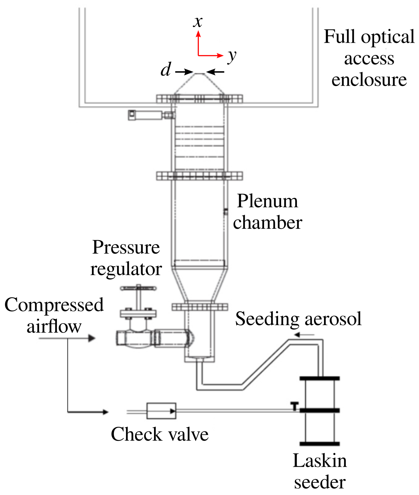
Abstract
1. Introduction
2. Experimental System
2.1. Jet Facility
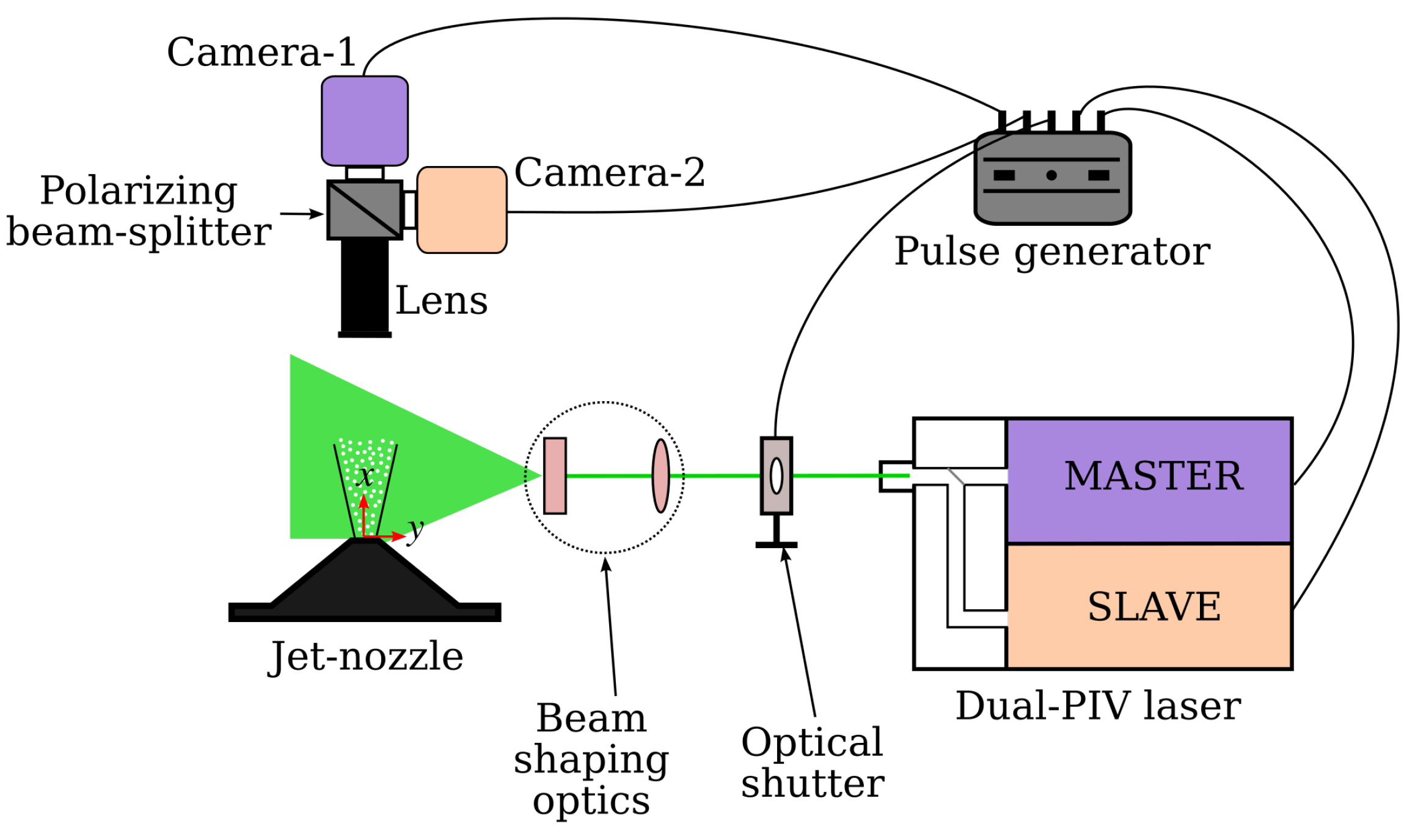
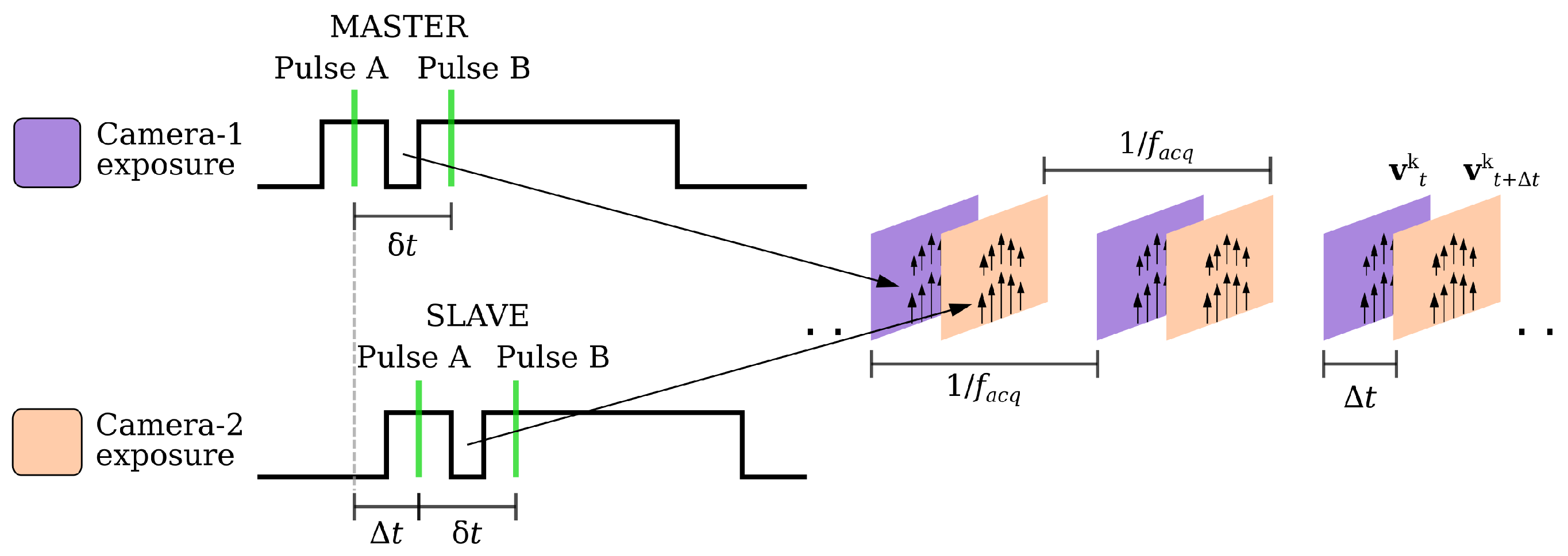
2.2. Dual-PIV
2.3. PIV Processing Algorithm
2.4. Measurement Uncertainties
3. Dynamic Mode Decomposition
- 1.
- Compute the singular value decomposition (SVD) of X
- 2.
- Truncate the SVD
- 3.
- Define the matrix
- 4.
- Perform eigenvalue decomposition of ( are the DMD eigenvalues)
- 5.
- Compute the eigenvalues of A
- 6.
- Compute the DMD modes
- 7.
- Compute the corresponding DMD modes amplitudes
4. Results
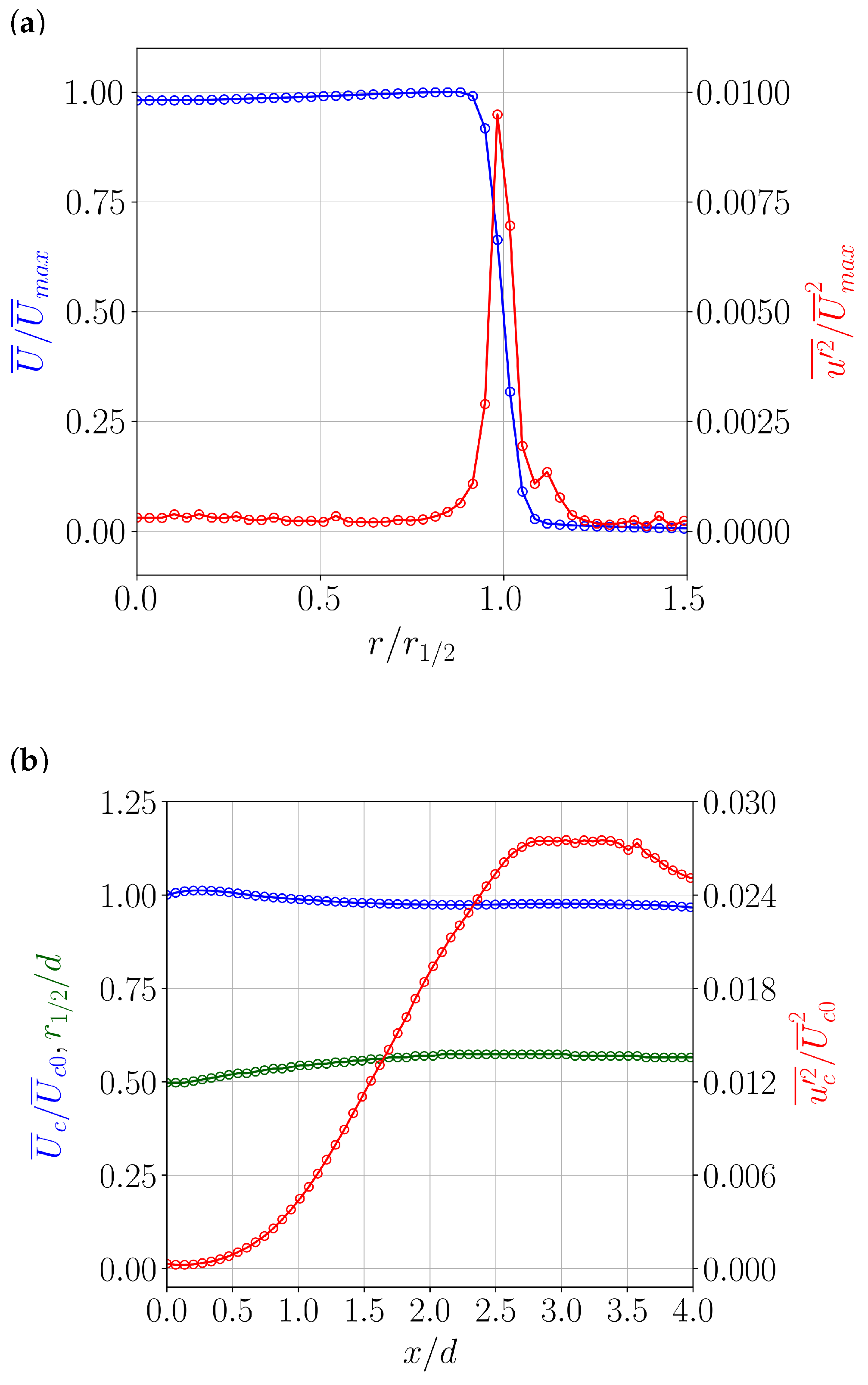
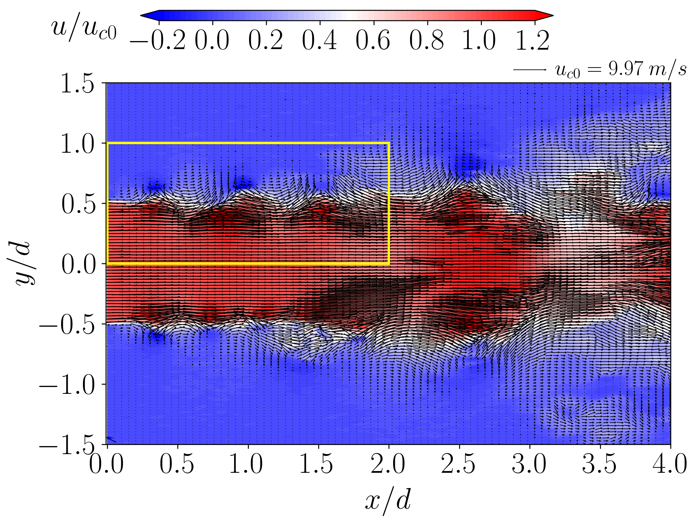
4.1. Jet Characterisation
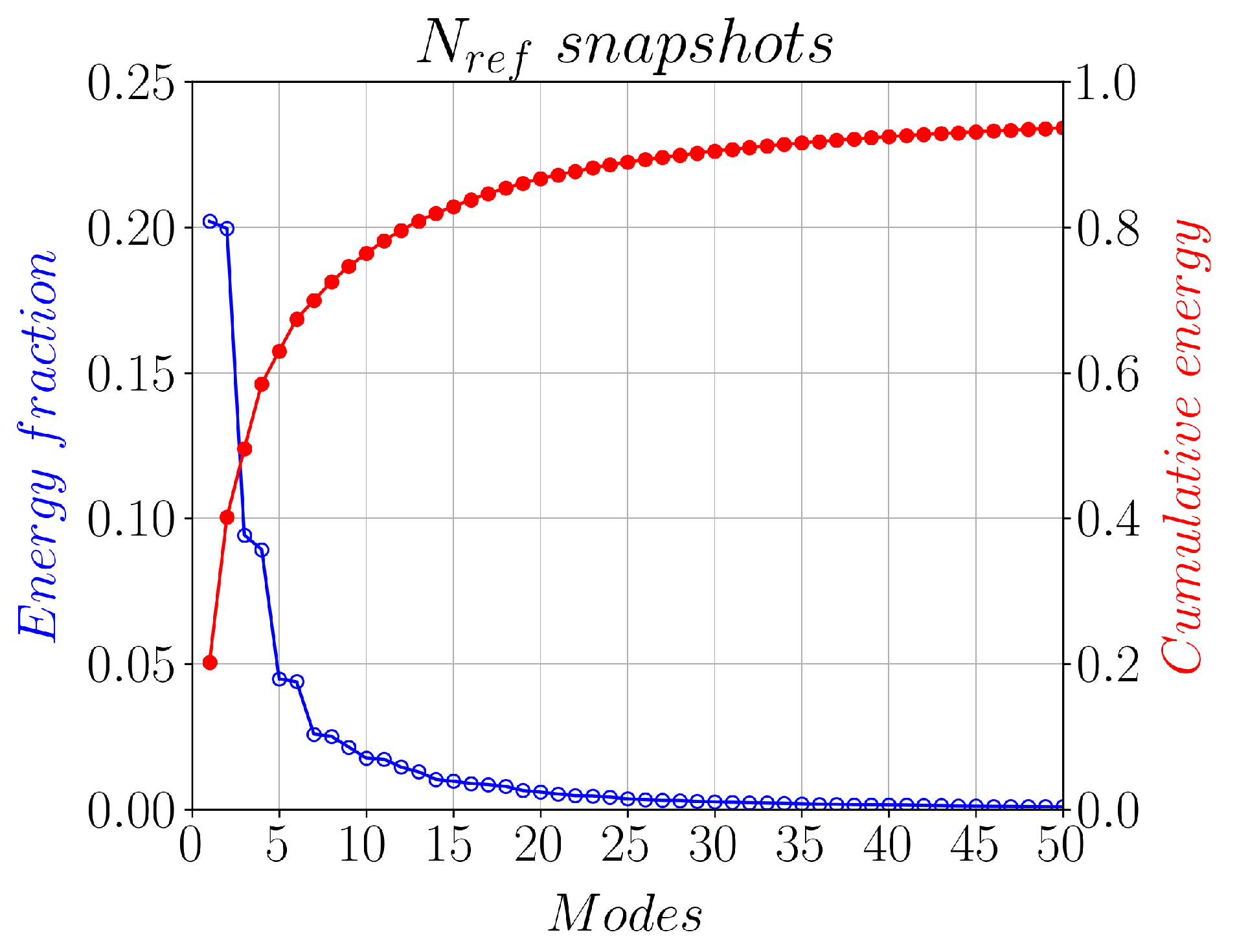
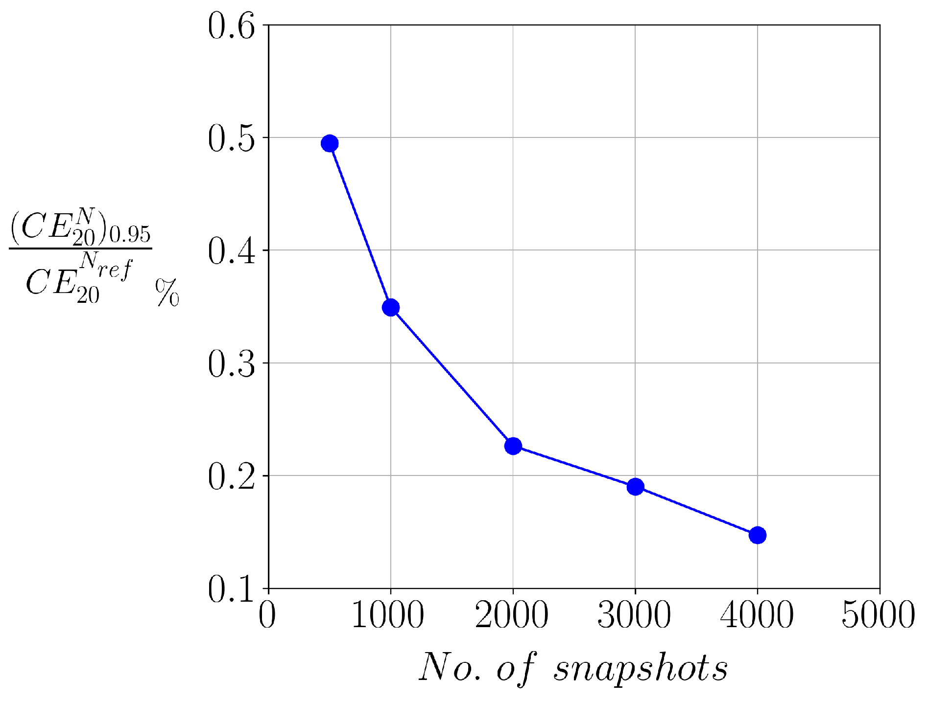
4.2. Assessment of Sample Size Sufficiency
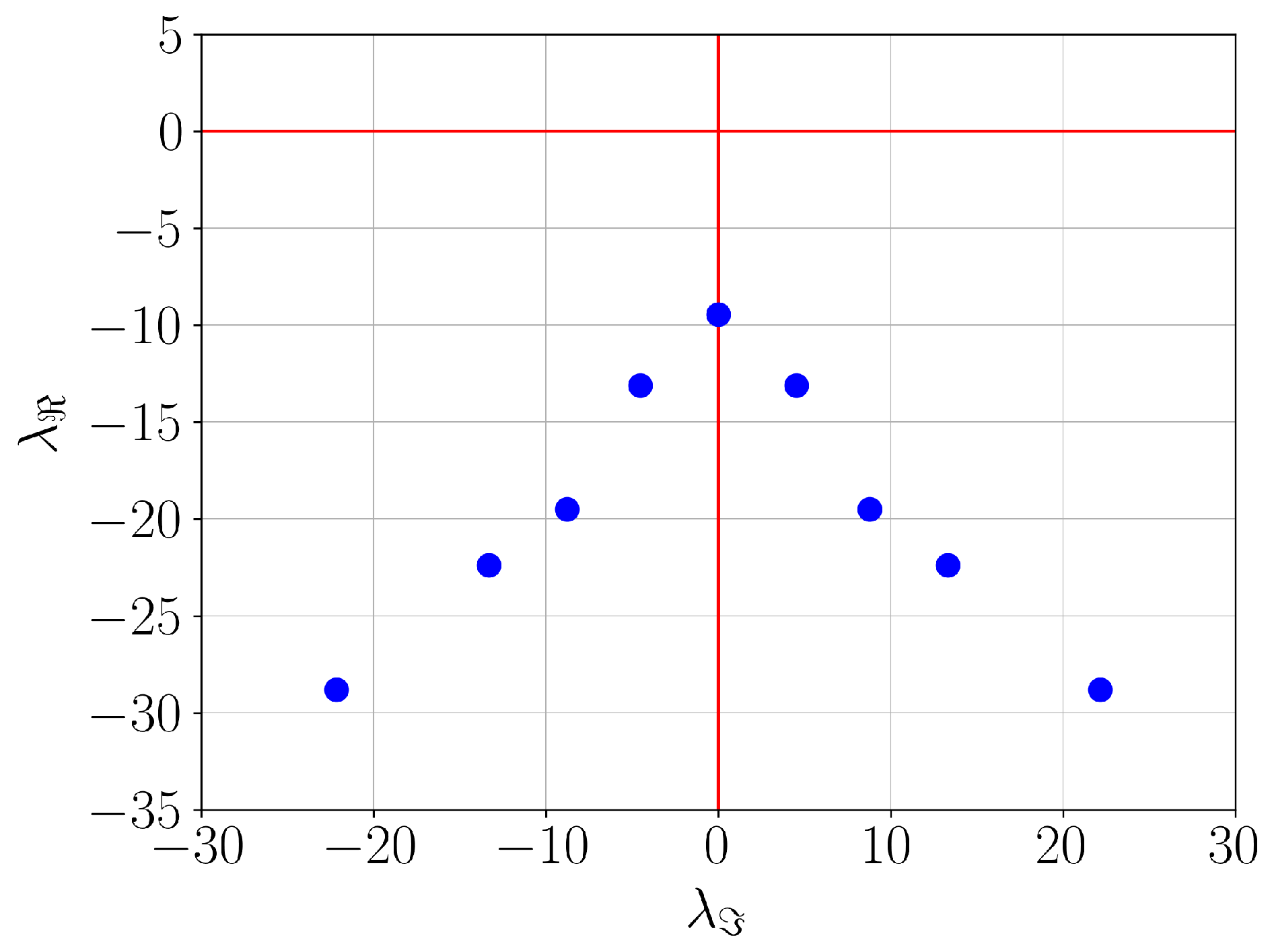
4.3. DMD Results
5. Discussion
6. Conclusions
Author Contributions
Funding
Data Availability Statement
Conflicts of Interest
Abbreviations
| DMD | Dynamic Mode Decomposition |
| PIV | Particle Image Velocimetry |
| SVD | Singular Value Decomposition |
References
- Edgington-Mitchell, D.; Oberleithner, K.; Honnery, D.R.; Soria, J. Coherent structure and sound production in the helical mode of a screeching axisymmetric jet. J. Fluid Mech. 2014, 748, 822–847. [Google Scholar] [CrossRef]
- Buchmann, N.A.; Duke, D.J.; Shakiba, S.A.; Mitchell, D.M.; Stewart, P.J.; Traini, D.; Young, P.M.; Lewis, D.A.; Soria, J.; Honnery, D. A novel high-speed imaging technique to predict the macroscopic spray characteristics of solution based pressurised metered dose inhalers. Pharm. Res. 2014, 31, 2963–2974. [Google Scholar] [CrossRef] [PubMed]
- Tong, C.; Warhaft, Z. Passive scalar dispersion and mixing in a turbulent jet. J. Fluid Mech. 1995, 292, 1–38. [Google Scholar] [CrossRef]
- Dimotakis, P.E. The mixing transition in turbulent flows. J. Fluid Mech. 2000, 409, 69–98. [Google Scholar] [CrossRef]
- Hu, H.; Saga, T.; Kobayashi, T.; Taniguchi, N. Analysis of a Turbulent Jet Mixing Flow by Using a PIV-PLIF Combined System. J. Vis. 2004, 7, 33–42. [Google Scholar] [CrossRef]
- Dahm, W.J.A.; Dimotakis, P.E. Measurements of entrainment and mixing in turbulent jets. AIAA J. 1987, 25, 1216–1223. [Google Scholar] [CrossRef]
- Bell, G.; Soria, J.; Honnery, D.; Edgington-Mitchell, D. An experimental investigation of coupled underexpanded supersonic twin-jets. Exp. Fluids 2018, 59, 139. [Google Scholar] [CrossRef]
- Edgington-Mitchell, D.; Jaunet, V.; Jordan, P.; Towne, A.; Soria, J.; Honnery, D. Upstream-travelling acoustic jet modes as a closure mechanism for screech. J. Fluid Mech. 2018, 855, R1. [Google Scholar] [CrossRef]
- Edgington-Mitchell, D.; Weightman, J.; Lock, S.; Kirby, R.; Nair, V.; Soria, J.; Honnery, D. The generation of screech tones by shock leakage. J. Fluid Mech. 2021, 908, A46. [Google Scholar] [CrossRef]
- Adrian, R.J. Particle-imaging techniques for experimental fluid mechanics. Annu. Rev. Fluid Mech. 1991, 23, 261–304. [Google Scholar] [CrossRef]
- Soria, J. Particle Image Velocimetry—Application to Turbulence Studies. In Lecture Notes on Turbulence and Coherent Structures in Fluids, Plasmas and Nonlinear Media; World Scientific: Singapore, 2006; pp. 309–347. [Google Scholar] [CrossRef]
- Scharnowski, S.; Kähler, C.J. Particle image velocimetry—Classical operating rules from today’s perspective. Opt. Lasers Eng. 2020, 135, 106185. [Google Scholar] [CrossRef]
- Khashehchi, M.; Ooi, A.; Soria, J.; Marusic, I. Evolution of the turbulent/non-turbulent interface of an axisymmetric turbulent jet. Exp. Fluids 2013, 54, 1449. [Google Scholar] [CrossRef]
- Qin, S.; Krohn, B.; Downing, J.; Petrov, V.; Manera, A. High-Resolution Velocity Field Measurements of Turbulent Round Free Jets in Uniform Environments. Nucl. Technol. 2019, 205, 213–225. [Google Scholar] [CrossRef]
- Weightman, J.L.; Amili, O.; Honnery, D.; Edgington-Mitchell, D.; Soria, J. Nozzle external geometry as a boundary condition for the azimuthal mode selection in an impinging underexpanded jet. J. Fluid Mech. 2019, 862, 421–448. [Google Scholar] [CrossRef]
- Fouras, A.; Soria, J. Accuracy of out-of-plane vorticity measurements derived from in-plane velocity field data. Exp. Fluids 1998, 25, 409–430. [Google Scholar] [CrossRef]
- Lavoie, P.; Avallone, G.; De Gregorio, F.; Romano, G.P.; Antonia, R.A. Spatial resolution of PIV for the measurement of turbulence. Exp. Fluids 2007, 43, 39–51. [Google Scholar] [CrossRef]
- Atkinson, C.; Buchmann, N.A.; Amili, O.; Soria, J. On the appropriate filtering of PIV measurements of turbulent shear flows. Exp. Fluids 2014, 55, 1654. [Google Scholar] [CrossRef]
- Wernet, M.P. Temporally resolved PIV for space-time correlations in both cold and hot jet flows. Meas. Sci. Technol. 2007, 18, 1387–1403. [Google Scholar] [CrossRef]
- Meslem, A.; El Hassan, M.; Nastase, I. Analysis of jet entrainment mechanism in the transitional regime by time-resolved PIV. J. Vis. 2011, 14, 41–52. [Google Scholar] [CrossRef]
- Semeraro, O.; Bellani, G.; Lundell, F. Analysis of time-resolved PIV measurements of a confined turbulent jet using POD and Koopman modes. Exp. Fluids 2012, 53, 1203–1220. [Google Scholar] [CrossRef]
- Breakey, D.E.; Fitzpatrick, J.A.; Meskell, C. Aeroacoustic source analysis using time-resolved PIV in a free jet. Exp. Fluids 2013, 54, 1531. [Google Scholar] [CrossRef]
- Miller, J.D.; Jiang, N.; Slipchenko, M.N.; Mance, J.G.; Meyer, T.R.; Roy, S.; Gord, J.R. Spatiotemporal analysis of turbulent jets enabled by 100-kHz, 100-ms burst-mode particle image velocimetry. Exp. Fluids 2016, 57, 192. [Google Scholar] [CrossRef]
- Berkooz, G.; Holmes, P.; Lumley, J.L. The Proper Orthogonal Decomposition in the Analysis of Turbulent Flows. Annu. Rev. Fluid Mech. 1993, 25, 539–575. [Google Scholar] [CrossRef]
- Chatterjee, A. An introduction to the proper orthogonal decomposition. Curr. Sci. 2000, 78, 808–817. [Google Scholar]
- Patte-Rouland, B.; Lalizel, G.; Moreau, J.; Rouland, E. Flow analysis of an annular jet by particle image velocimetry and proper orthogonal decomposition. Meas. Sci. Technol. 2001, 12, 1404. [Google Scholar] [CrossRef]
- Bi, W.; Sugii, Y.; Okamoto, K.; Madarame, H. Time-resolved proper orthogonal decomposition of the near-field flow of a round jet measured by dynamic particle image velocimetry. Meas. Sci. Technol. 2003, 14, L1. [Google Scholar] [CrossRef]
- Tinney, C.E.; Glauser, M.N.; Ukeiley, L.S. Low-dimensional characteristics of a transonic jet. Part 1. Proper orthogonal decomposition. J. Fluid Mech. 2008, 612, 107–141. [Google Scholar] [CrossRef]
- Shinneeb, A.M.; Balachandar, R.; Bugg, J.D. Analysis of coherent structures in the far-field region of an axisymmetric free jet identified using particle image velocimetry and proper orthogonal decomposition. J. Fluids Eng. Trans. ASME 2008, 130, 011202. [Google Scholar] [CrossRef]
- He, C.; Liu, Y. Proper orthogonal decomposition-based spatial refinement of TR-PIV realizations using high-resolution non-TR-PIV measurements. Exp. Fluids 2017, 58, 86. [Google Scholar] [CrossRef]
- Ozawa, Y.; Nagata, T.; Nishikori, H.; Nonomura, T.; Asai, K. POD-based Spatio-temporal Superresolution Measurement on a Supersonic Jet using PIV and Near-field Acoustic Data. In Proceedings of the AIAA AVIATION 2021 Forum; American Institute of Aeronautics and Astronautics Inc., AIAA: Reston, VA, USA, 2021. [Google Scholar] [CrossRef]
- Price, T.J.; Gragston, M.; Kreth, P.A. Supersonic underexpanded jet features extracted from modal analyses of high-speed optical diagnostics. AIAA J. 2021, 59, 4917–4934. [Google Scholar] [CrossRef]
- Taira, K.; Brunton, S.L.; Dawson, S.T.; Rowley, C.W.; Colonius, T.; McKeon, B.J.; Schmidt, O.T.; Gordeyev, S.; Theofilis, V.; Ukeiley, L.S. Modal analysis of fluid flows: An overview. AIAA J. 2017, 55, 4013–4041. [Google Scholar] [CrossRef]
- Schmid, P.J. Dynamic mode decomposition of numerical and experimental data. J. Fluid Mech. 2010, 656, 5–28. [Google Scholar] [CrossRef]
- Schmid, P.J.; Li, L.; Juniper, M.P.; Pust, O. Applications of the dynamic mode decomposition. Theor. Comput. Fluid Dyn. 2010, 25, 249–259. [Google Scholar] [CrossRef]
- Schmid, P.J.; Violato, D.; Scarano, F. Decomposition of time-resolved tomographic PIV. Exp. Fluids 2012, 52, 1567–1579. [Google Scholar] [CrossRef]
- Ozawa, Y.; Nishikori, H.; Nagata, T.; Nonomura, T.; Asai, K.; Colonius, T. DMD-based Superresolution Measurement of a Supersonic Jet using Dual Planar PIV and Acoustic Data. In Proceedings of the 28th AIAA/CEAS Aeroacoustics Conference; American Institute of Aeronautics and Astronautics Inc., AIAA: Reston, VA, USA, 2022. [Google Scholar] [CrossRef]
- Fontaine, R.A.; Elliott, G.S.; Austin, J.M.; Freund, J.B. Very near-nozzle shear-layer turbulence and jet noise. J. Fluid Mech. 2015, 770, 27–51. [Google Scholar] [CrossRef]
- Tu, J.H.; Rowley, C.W.; Luchtenburg, D.M.; Brunton, S.L.; Kutz, J.N. On dynamic mode decomposition: Theory and applications. J. Comput. Dyn. 2014, 1, 391–421. [Google Scholar] [CrossRef]
- Guibert, P.; Lemoyne, L. Dual particle image velocimetry for transient flow field measurements. Exp. Fluids 2002, 33, 355–367. [Google Scholar] [CrossRef]
- Wernet, M.P.; John, W.T.; Bridges, J. Dual PIV Systems for Space-Time Correlations in Hot Jets. In Proceedings of the 20th International Congress on Instrumentation in Aerospace Simulation Facilities, Gottingen, Germany, 25–29 August 2003; pp. 127–135. [Google Scholar] [CrossRef]
- Pinier, J.T.; Glauser, M.N. Dual-Time PIV Investigation of the Sound Producing Region of the High-Speed Jet. In Proceedings of the 37th AIAA Fluid Dynamics Conference and Exhibit, Miami, FL, USA, 25–28 June 2007. [Google Scholar] [CrossRef]
- Schreyer, A.M.; Lasserre, J.J.; Dupont, P. Development of a Dual-PIV system for high-speed flow applications. Exp. Fluids 2015, 56, 187. [Google Scholar] [CrossRef]
- Soria, J.; Amili, O. Under-expanded impinging supersonic jet flow. In Proceedings of the 10th Pacific Symposium on Flow Visualization and Image Processing, Naples, Italy, 15–18 June 2015; pp. 15–18. [Google Scholar]
- Weightman, J.L.; Amili, O.; Honnery, D.; Soria, J.; Edgington-Mitchell, D. An explanation for the phase lag in supersonic jet impingement. J. Fluid Mech. 2017, 815, R1. [Google Scholar] [CrossRef]
- Sikroria, T.; Sandberg, R.; Ooi, A.; Karami, S.; Soria, J. Investigating Shear-Layer Instabilities in Supersonic Impinging Jets Using Dual-Time Particle Image Velocimetry. AIAA J. 2022, 60, 3749–3759. [Google Scholar] [CrossRef]
- Christensen, K.T.; Adrian, R.J. Measurement of instantaneous Eulerian acceleration fields by particle image accelerometry: Method and accuracy. Exp. Fluids 2002, 33, 759–769. [Google Scholar] [CrossRef]
- Kähler, C.J. Investigation of the spatio-temporal flow structure in the buffer region of a turbulent boundary layer by means of multiplane stereo PIV. Exp. Fluids 2004, 36, 114–130. [Google Scholar] [CrossRef]
- Souverein, L.J.; Van Oudheusden, B.W.; Scarano, F.; Dupont, P. Application of a dual-plane particle image velocimetry (dual-PIV) technique for the unsteadiness characterization of a shock wave turbulent boundary layer interaction. Meas. Sci. Technol. 2009, 20, 074003. [Google Scholar] [CrossRef]
- Liu, X.; Katz, J. Instantaneous pressure and material acceleration measurements using a four-exposure PIV system. Exp. Fluids 2006, 41, 227–240. [Google Scholar] [CrossRef]
- Sikroria, T. Investigation of the Shear-Layer Instabilities in Supersonic Impinging Jets Using Dual-Time Velocity Measurements. Ph.D. Thesis, The University of Melbourne, Melbourne, Australia, 2021. [Google Scholar]
- Fedrizzi, M.; Soria, J. Application of a single-board computer as a low-cost pulse generator. Meas. Sci. Technol. 2015, 26, 095302. [Google Scholar] [CrossRef]
- Ho, C.M.; Huerre, P. Perturbed free shear layers. Annu. Rev. Fluid Mech. 1984, 16, 365–424. [Google Scholar] [CrossRef]
- Soria, J. Digital cross-correlation particle image velocimetry measurements in the near wake of a circular cylinder. In Proceedings of the International Colloquium on Jets, Wakes and Shear Layers, CSIRO Australia, Melbourne, Australia, 18–20 April 1994; pp. 21–25. [Google Scholar]
- Soria, J. An investigation of the near wake of a circular cylinder using a video-based digital cross-correlation particle image velocimetry technique. Exp. Therm. Fluid Sci. 1996, 12, 221–233. [Google Scholar] [CrossRef]
- Soria, J.; New, T.H.; Lim, T.T.; Parker, K. Multigrid CCDPIV measurements of accelerated flow past an airfoil at an angle of attack of 30°. Exp. Therm. Fluid Sci. 2003, 27, 667–676. [Google Scholar] [CrossRef]
- Hart, D.P. PIV error correction. Exp. Fluids 2000, 29, 13–22. [Google Scholar] [CrossRef]
- Westerweel, J.; Scarano, F. Universal outlier detection for PIV data. Exp. Fluids 2005, 39, 1096–1100. [Google Scholar] [CrossRef]
- Soria, J. Effect of velocity gradients on 3D cross-correlation PIV analysis and the calculation of the velocity gradient tensor. In Proceedings of the 14th International Symposium on Applications of Laser Techniques to Fluid Mechanics, Lisbon, Portugal, 7–10 July 2008. [Google Scholar]
- Soria, J. Multigrid approach to cross-correlation digital PIV and HPIV analysis. In Proceedings of the 13th Australasian Fluid Mechanics Conference, Monash University. Melbourne, Australia, 13–18 December 1998; pp. 381–384. [Google Scholar]
- Sikroria, T.; Soria, J.; Karami, S.; Sandberg, R.D.; Ooi, A. Measurement and analysis of the shear-layer instabilities in supersonic impinging jets using dual-time velocity data. In AIAA AVIATION 2020 FORUM; American Institute of Aeronautics and Astronautics: Reston, VA, USA, 2020; Volume 1, Part F. [Google Scholar] [CrossRef]
- Sarmast, S.; Dadfar, R.; Mikkelsen, R.F.; Schlatter, P.; Ivanell, S.; Sørensen, J.N.; Henningson, D.S. Mutual inductance instability of the tip vortices behind a wind turbine. J. Fluid Mech. 2014, 755, 705–731. [Google Scholar] [CrossRef]
- Michalke, A.; Hermann, G. On the inviscid instability of a circular jet with external flow. J. Fluid Mech. 1982, 114, 343–359. [Google Scholar] [CrossRef]
- Freymuth, P. On transition in a separated laminar boundary layer. J. Fluid Mech. 1966, 25, 683–704. [Google Scholar] [CrossRef]


Disclaimer/Publisher’s Note: The statements, opinions and data contained in all publications are solely those of the individual author(s) and contributor(s) and not of MDPI and/or the editor(s). MDPI and/or the editor(s) disclaim responsibility for any injury to people or property resulting from any ideas, methods, instructions or products referred to in the content. |
© 2023 by the authors. Licensee MDPI, Basel, Switzerland. This article is an open access article distributed under the terms and conditions of the Creative Commons Attribution (CC BY) license (https://creativecommons.org/licenses/by/4.0/).
Share and Cite
Chaugule, V.; Duddridge, A.; Sikroria, T.; Atkinson, C.; Soria, J. Investigating the Linear Dynamics of the Near-Field of a Turbulent High-Speed Jet Using Dual-Particle Image Velocimetry (PIV) and Dynamic Mode Decomposition (DMD). Fluids 2023, 8, 73. https://doi.org/10.3390/fluids8020073
Chaugule V, Duddridge A, Sikroria T, Atkinson C, Soria J. Investigating the Linear Dynamics of the Near-Field of a Turbulent High-Speed Jet Using Dual-Particle Image Velocimetry (PIV) and Dynamic Mode Decomposition (DMD). Fluids. 2023; 8(2):73. https://doi.org/10.3390/fluids8020073
Chicago/Turabian StyleChaugule, Vishal, Alexis Duddridge, Tushar Sikroria, Callum Atkinson, and Julio Soria. 2023. "Investigating the Linear Dynamics of the Near-Field of a Turbulent High-Speed Jet Using Dual-Particle Image Velocimetry (PIV) and Dynamic Mode Decomposition (DMD)" Fluids 8, no. 2: 73. https://doi.org/10.3390/fluids8020073
APA StyleChaugule, V., Duddridge, A., Sikroria, T., Atkinson, C., & Soria, J. (2023). Investigating the Linear Dynamics of the Near-Field of a Turbulent High-Speed Jet Using Dual-Particle Image Velocimetry (PIV) and Dynamic Mode Decomposition (DMD). Fluids, 8(2), 73. https://doi.org/10.3390/fluids8020073