1. Introduction
Atmospheric convection involves the vertical transport of heat and moisture into the unstable atmosphere. This mechanism is key to the formation of clouds and atmospheric circulation and it redistributes heat and moisture from warm equatorial regions to higher latitudes. The interaction between the atmosphere and oceans is pronounced in the tropics compared to other regions. India, being a tropical country, and with water mass surrounding the sub-continent, is more prone to convective activities. Over the Bay of Bengal (BoB), these activities are especially more frequent [
1] and studies have highlighted the dynamics of the convection phenomenon over the Bay of Bengal [
2,
3]. These processes are understood better with observational data, but having observations at each and every point is not feasible. Thus, computational studies are used as tools to generate data similar to observations. Large-scale models, such as the general circulation models (GCMs) and regional circulation models (RCMs), have grid resolutions that are too coarse to resolve the convective and cloud-scale processes, and hence these sub-grid-scale processes need to be parameterized. With an increase in computational resources, high-resolution models (e.g., cloud-resolving LES) can be used to parametrize these sub-grid-scale processes for a given large-scale forcing and sounding. One of the important factors for the parametrization, as pointed out by many studies, is the entrainment rate [
4,
5]. It is an important factor that affects the development of clouds and is defined as the mixing of the environmental air into clouds. Such dynamics are, however, not properly simulated in GCMs and are represented statistically.
In the present work, the Bay of Bengal has been chosen as the region of interest, as it represents an essential source of moisture for Asian monsoons. A recent computational study incorporating the regional-scale model [
6] has investigated the thermodynamic structure of large-scale convective systems, which propagate towards the equator. However, the simulation of cloud-scale processes is a challenge for many atmospheric global and regional models as convection processes are parametrized and are not resolved in these models [
7,
8]. The reported studies did not resolve the small-scale processes leading to the formation of clouds, and these processes can be resolved using high-resolution models. The performance of such studies becomes essential for the region, to better understand the parameterization of convection physics and the model biases over the region.
The high-resolution models can be used to simulate the convective processes. The capability of Large Eddy Simulation (LES) models to resolve convection, clouds, and boundary-layer turbulence is well established [
9,
10,
11,
12,
13,
14]. The reported LES studies have mostly been based on field campaigns that were performed on selected locations, such as BOMEX [
7], DYCOMS-II [
15], and RICO [
16]. Therefore, in order to understand the convection phenomenon, we designed the LES for simulating convection over the Bay of Bengal. An experimental study on the BoB was conducted by Bhat et al. [
1] as part of the Indian Climate Research Programme in July-August 1999. This effort, known by its abbreviation BOBMEX, focused mainly on the measurement of important atmospheric and oceanic variables, as well as fluxes, to gain a deeper insight into the convection phenomenon. However, the data obtained from BOBMEX were insufficient to drive an LES model since advective tendencies cannot be derived explicitly from such data. Thus, an alternative way of driving LES from reanalysis data was used in the present study.
We describe an LES experiment that was forced through the initial and boundary conditions from ERA5 (Fifth Generation European Centre for Medium-Range Weather Forecast Atmospheric Reanalysis) [
17] data. The time and location of the input conditions forced on the LES were the same as those of BOBMEX and therefore the synoptic-scale and mesoscale conditions are represented well in the LES. As the computational domain for LES is smaller than the size of the synoptic-scale activity, the implication here is that the LES only gives sub-mesoscale information, which is essentially small-scale detail on the top of the mean coarser-scale information in which the LES resides. Within the scope of the present work, we focused on gaining an understanding of the weak phase of convection. The weak phase of convection has high outgoing longwave radiation (OLR) values, winds with low speed, and a low cloud cover. The convection occurring during weak phases serves as an essential component that contributes to the development of the deep convective activity. The atmospheric turbulence has been mostly studied using high-frequency observational data [
18,
19]. In the present work, turbulence properties of convection were comprehended by applying Reynoldsaveraging [
20] to the model output. The turbulent fluctuations, along with their variances and covariances, were indicative of the convective turbulence strength. In the present study, we also employed Reynolds averaging to estimate the turbulence strength throughout the region during the weak convection phase. Additionally, we also investigated the properties of clouds and entrainment rate by conditionally averaging the model output.
2. Methodology
A simulation using the LES model is initialized using initial and boundary conditions. The initial conditions include vertical profiles of temperature, moisture, and winds. The boundary conditions include surface conditions, sea surface temperature, surface fluxes, and large-scale forcings, i.e., large-scale advection and subsidence [
16]. These initial and boundary conditions are mostly based on observational studies. However, in the present study, the LES model was driven by the conditions generated from ERA5 reanalysis data. The present LES study was carried out by using Cloud Model 1 (CM1) version 20.2, NCAR, Boulder, USA. CM1 is a fully nonlinear, compressible, and non-hydrostatic atmospheric model. CM1 integrates the governing equations for
u,
v,
w,
π’,
θ’, and
qx where
π is non-dimensional pressure,
qx is the mixing ratio for the moisture variables, and
θ denotes potential temperature [
21,
22]. The governing equations for
u,
v, and
w may be written as
In Equations (1)–(3), ADV denotes the advection, T represents the tendencies from the sub-grid-scale turbulence, D represents tendencies from other diffusive processes and does not include sub-grid-scale turbulence, N denotes the Newtonian relaxation terms, B the buoyancy term, and f represents the Coriolis acceleration.
The simulations were performed over a domain size of 25 km × 25 km × 25 km in the x, y, and z directions, respectively, using a standard uniform horizontal grid spacing of Δx = Δy = 100 m and, with a uniform grid size Δz = 50 m up to 5 km, followed by a uniformly stretched grid from 50 m to 200 m up to the height of 15 km, and then constant grid size of 200 m to domain top in the vertical direction. Doubly periodic boundary conditions were used for the lateral boundary, while the top and bottom boundary conditions were kept as free slip and semi-slip, respectively. The semi-slip condition is a modified form of the no-slip condition in which the surface roughness is specified at the boundary. The horizontal grid size of the LES in the present study was 100 m; therefore, large energy-containing eddies greater than 100 m were mostly resolved, while smaller sub-grid eddies were parametrized. The turbulence kinetic energy model was used for parameterizing the sub-grid-scale processes. In this model, turbulence kinetic energy is predicted, which is then used to determine the eddy viscosity (Km) and eddy diffusivity (Kh) that are required for modeling the sub-grid processes.
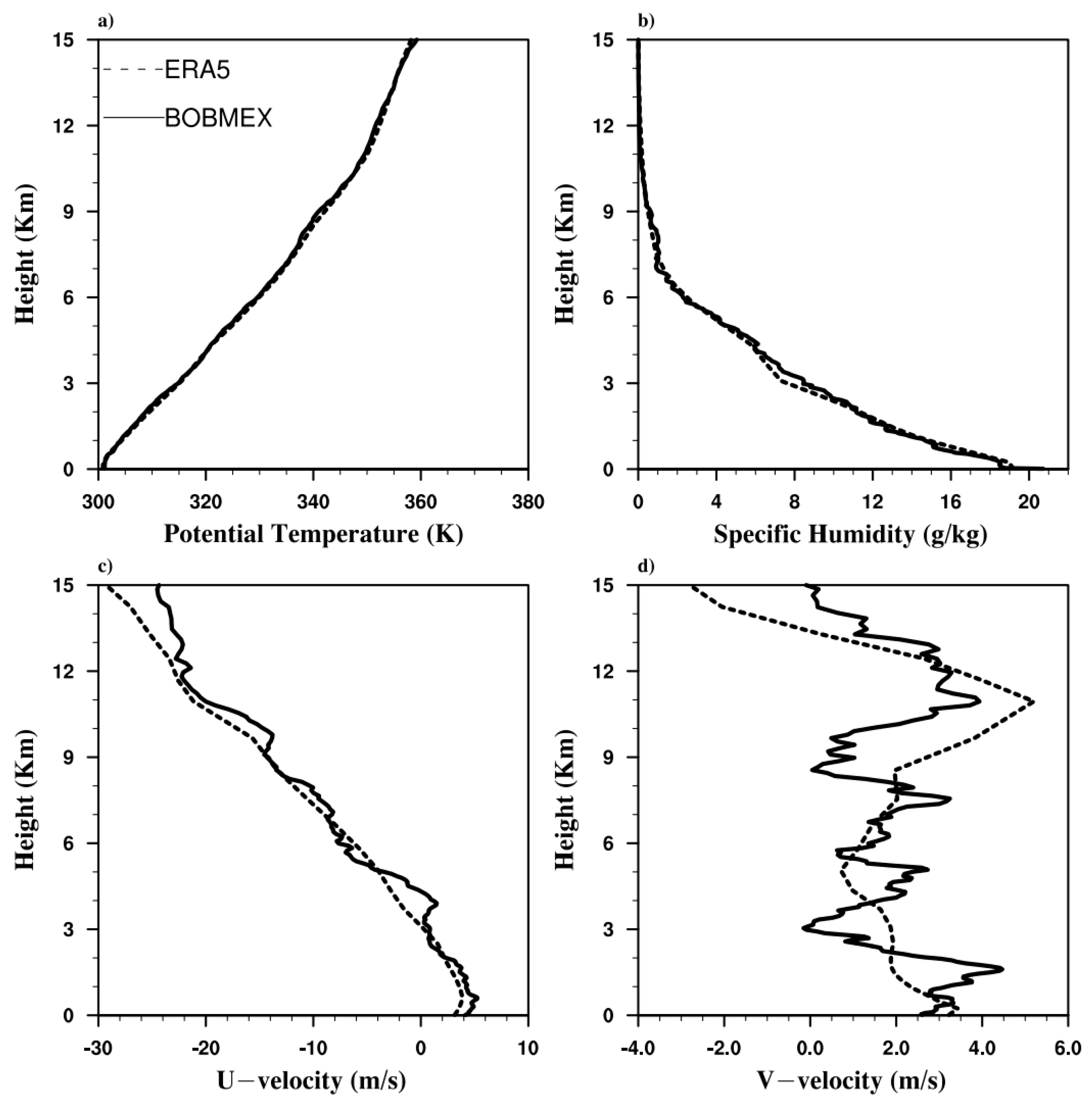
The simulations were performed for 18 h with an adaptive time step of 3 s. The sea surface temperature was kept fixed to 301.7 K. Before initializing the LES model, initial conditions from the ERA5 data needed to be validated against the observation data from the Bay of Bengal Monsoon Experiment (BOBMEX). BOBMEX was a ship-based observational study carried over the Bay of Bengal during the year 1999. High-resolution atmospheric data were measured by launching radiosondes from the ship. Typically, 2–5 radiosondes per day were launched with a resolution of approximately 25–30 m [
1]. The atmospheric state profiles were for the weak convection day [
1] over the Bay of Bengal on the 22nd of August 1999 and were averaged over a 24 h period. The values from INSAT of OLR during this day were high and the surface wind speed measured from the buoys was low [
1]. A comparison of initial profiles of potential temperature, specific humidity, and
u and
v velocity from ERA5 and BOBMEX is shown in
Figure 1. The ERA5 profiles of potential temperature and specific humidity were comparable to the observational data, although the mid-troposphere specific humidity profile was slightly less humid compared to the observational data. The weak convective day also had weak horizontal winds, and this was also illustrated by the low magnitudes of the
u and
v velocity wind profiles, as shown in
Figure 1c,d. The vertical profile of
u velocity from ERA5 was nearly similar to the observational data, while for the
v velocity, the trend was similar. As a whole, the averaged profiles of the ERA5 data were a reasonable representation of the mean profiles and consistent with the observational data; therefore, these can be used for performing LES.
3. Results
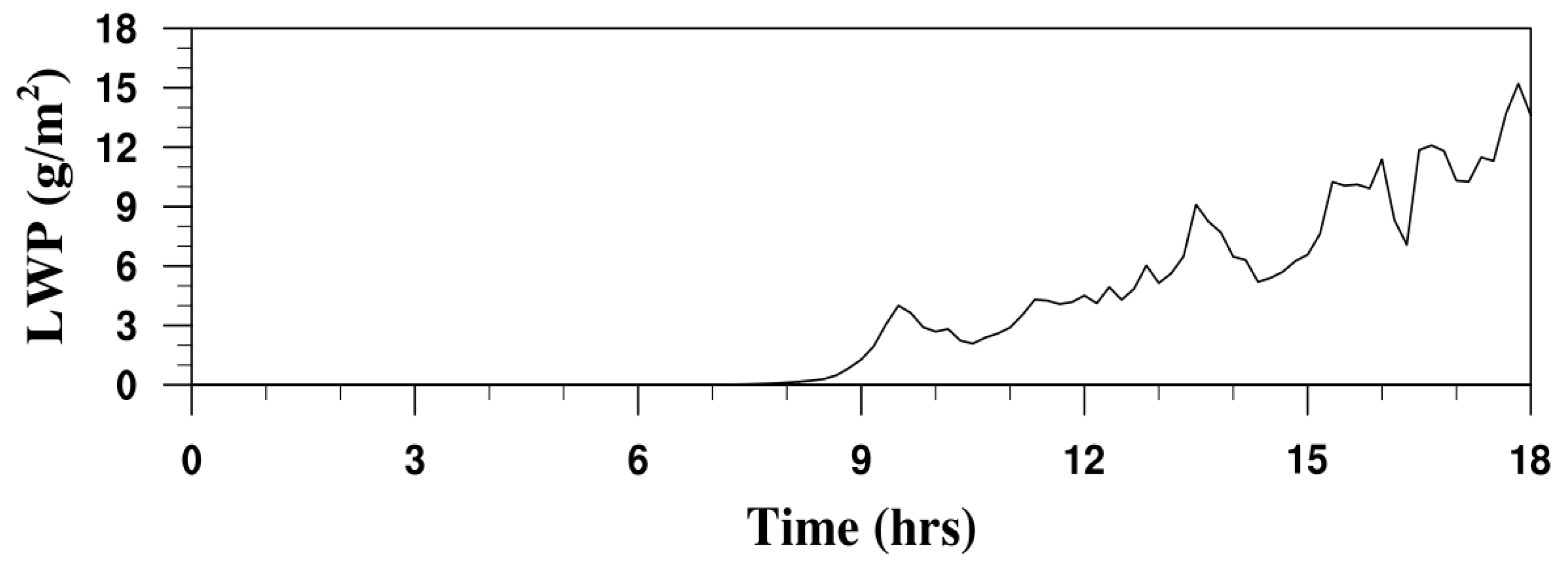
The results obtained from the LES are discussed in this section. The time evolution of the domain-averaged liquid water path for simulations has been illustrated in
Figure 2. The evolution of the liquid water path demonstrated that it was unquestionably a case of weak convection. This was evident from the fact that there was no cloud formation during the first seven to eight hours. Then, beginning at the eighth hour, there was a formation of liquid water, although the magnitude of it was still quite low. Liquid water path values in the range of 10–15 g/m
2 demonstrated the development of shallow cumulus clouds. Shallow cumulus clouds are low-height, non-precipitating, and basically the type that form on fair weather days. These clouds have a low liquid water content, their depth ranges from 1–2 km, and they have a shorter life span.
The observation of the horizontally averaged cloud liquid water content, as shown in
Figure 3, lent support to the hypothesis that shallow cumulus clouds were formed. Approximately 7 h after the simulation, clouds began to develop, and by the end of the experiment they reached a height of more than 2 km. The bases of the clouds that were generated remained the same while the height of the cloud tops grew. These types of clouds are typically classified as shallow cumulus clouds.
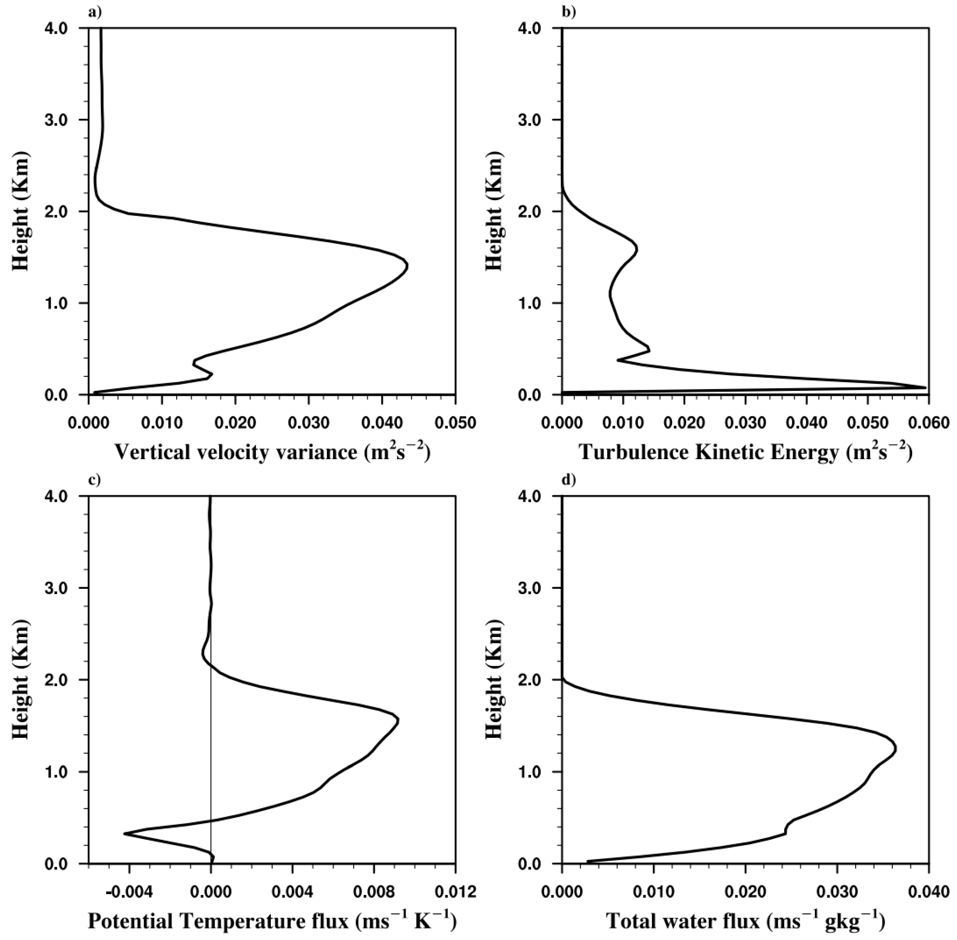
Turbulence is an important part of the atmosphere and can be studied by quantifying it. The vertical velocity variance, turbulence kinetic energy, and fluxes of moisture and temperature were used to analyze the turbulence properties of the simulation, and the results are shown in
Figure 4. The profiles were an average of the last two hours of the simulation when the clouds reached their steady height. The vertical velocity variance and the turbulence kinetic energy (TKE) are measures of the turbulence intensity, and the fluxes were determined by the covariance of the temperature and the moisture. Reynolds averaging was performed over the vertical velocity wind component to obtain the mean and turbulence parts in order to calculate the vertical velocity variance as shown below [
20].
where the overbar represents the mean of variable, and the prime indicates the fluctuating quantity. Similarly,
TKE was obtained from the sum of variances of all the three components of wind velocity.
The turbulent fluxes of temperature and moisture were obtained from the covariance of two variables
and
as:
The profile of vertical velocity variance revealed a double-peak structure, with the smaller peak located near the cloud base and the larger peak located towards the cloud top (
Figure 4a). Its magnitude was modest compared to that obtained by Siebesma et al. (2003), and the present low value indicates less intense turbulence, confirming its classification as weak convection. Compared to the sub-cloud layer, cloudy regions had lower values of turbulence kinetic energy (
Figure 4b). This lower value in the cloudy zone also showed that the convection over the domain was weak, whereas larger values in the sub-cloud layer may be attributable to the horizontal winds (
Figure 4).
The turbulent flux of potential temperature, which is calculated from the covariances of vertical velocity and potential temperature, had a positive value in the cloudy region, which indicated that both w and θ tended to vary in the same direction (positive/negative) on average. However, this value was negative below the cloud base and near the cloud top, which indicated that these two variables varied in the opposite direction. Moreover, the turbulent flux of water showed an overall positive value till the cloud top. The magnitude of the fluxes was low, which meant that there were only a few locations where clouds were observed over the domain. Thus, it can be considered as a case of weak convection.
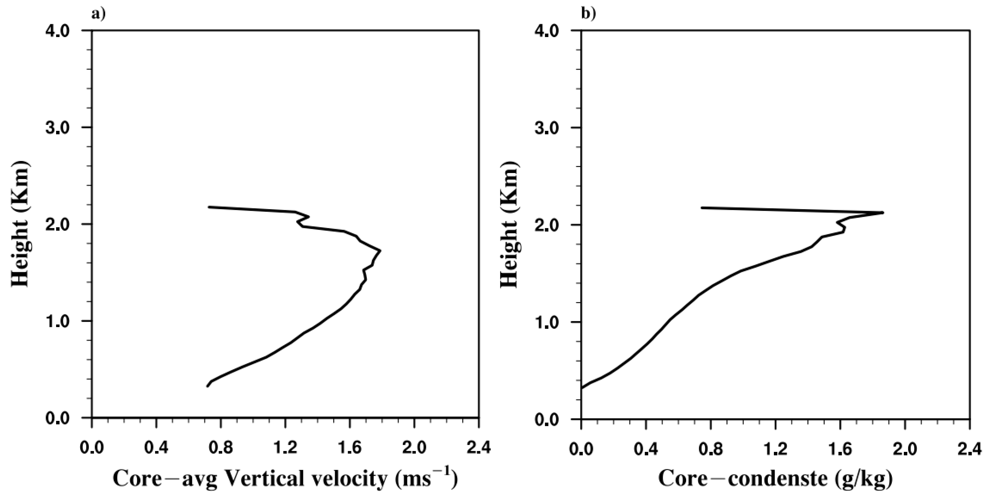
Despite the fact that the simulation was run for the situation of a weak convection, it was still possible to investigate the structure of the clouds that were created over the domain by conditionally averaging the output. The grid points that have a positive liquid water content and vertical velocity are referred to as the core of the cloud [
9,
23]. The profiles of the cloud core vertical velocity and liquid water as cloud condensate are shown in
Figure 5. The shallow cumulus clouds were formed over the domain in the simulation. It can be inferred from
Figure 5 that the properties of the cloud cores formed in the present simulation were similar to those reported in the literature [
9]. The fact that the cores had a significant amount of vertical velocity and a high liquid water content validated the creation of clouds because it demonstrated that the cloud core parameters were consistent with the previous research.
The entrainment rate was one of the critical factors in the parametrization. It was obtained from the LES by using the simple bulk plume approach in which the ensemble of clouds was considered for the transport of heat and moisture. The entrainment rate was calculated by the simple entraining plume model [
24,
25,
26] as
where
represents a conserved variable, i.e., total water, and subscript
c represents the cloud core, and
represents the entrainment rate. Variation in the entrainment rate with height from the simulation is shown in
Figure 6. The value of the entrainment rate decreased with height, with the maximum value around the cloud base, and this trend was consistent with the reported literature. The entrainment rate was slightly higher near the cloud base in the present simulation than that obtained by Siebesma et al. [
9] and this increased value enhanced the mixing of the surrounding air into the cloud, thus limiting the cloud height.
4. Discussion
The vertical movement of heat and moisture into the atmosphere is an essential part of the atmospheric convection process. In the context of India, the Bay of Bengal region is more susceptible to these convective events than the other parts of the country. These activities are better understood with the observational data. However, in the present work, we have studied the feature of atmospheric convection over the Bay of Bengal numerically by performing a large eddy simulation, which is an advanced technique for studying fluid turbulence. This was done so that we could gain additional knowledge about the characteristics of atmospheric convection. The generation of accurate initial and boundary conditions is a key part of properly carrying out a LES of a turbulent flow. In order to coerce LES into simulating the turbulent convection, we successfully derived the initial and boundary conditions from the reanalysis data. The present LES was able to simulate convection quite accurately, as seen by the appearance of shallow cumulus clouds over the region under investigation. Further, the turbulence characteristics and cloud dynamics features, which were mostly obtained in the literature through flight observations, were also analyzed using the present LES output. This was done in order to better understand the relationship between the two. The simulated convection feature mostly depended on the scales resolved by LES. However, due to the constraints of the computational resources, we carried out LES with a horizontal grid size of 100 m. We recommend performing LES in the future using a better resolution in order to assess the sensitivity of the results.
5. Conclusions
A large eddy simulation (LES) of atmospheric convection was carried out for the Bay of Bengal region during the weak convection phase. The LES model was forced with initial and boundary conditions from the ERA5 reanalysis data. The ERA5 data was verified against the observational data, and the profiles were found to be analogous to the observations. The simulation was carried out for a time period of 18 h over a domain size of 25 km × 25 km × 25 km in the x, y, and z directions, respectively, using a uniform horizontal grid spacing of Δx = Δy = 100 m and, with a uniform grid size of Δz = 50 m up to 5 km, followed by a uniformly stretched grid from 50 m to 200 m up to the height of 15 km, and then a uniform grid size of 200 m up to the domain top in the vertical direction. The time evolution of the liquid water path (LWP) showed that clouds were formed after 7–8 h of the simulation, and the clouds formed were shallow cumulus in nature as the LWP values were in the range of 10–15 g/m2. As the cloud tops reached a height of approximately 2 km, the horizontally averaged contour plots of the evolving contour also indicated that the clouds created were shallow cumulus. The turbulence characteristics obtained by the Reynolds averaging of the model output showed the presence of turbulence over the region. However, the intensity of turbulence was weak compared to that reported in the literature, and this fact supported the presence of weak convection. The cloud characteristics of simulation obtained from the conditionally averaged model output fields showed that the clouds formed had characteristics similar to those reported in other studies. The entrainment rate obtained was slightly higher near the cloud base than was the case in the reported literature. Thus, it can be concluded that the LES successfully simulated weak convection with its turbulence characteristics. The present study paves a pathway to perform various simulations at different atmospheric conditions over the region in order to create a library of high-resolution simulations.


