Abstract
For weakly nonlinear waves in one space dimension, the nonlinear Schrödinger Equation is widely accepted as a canonical model for the evolution of wave groups described by modulation instability and its soliton and breather solutions. When there is forcing such as that due to wind blowing over the water surface, this can be supplemented with a linear growth term representing linear instability leading to the forced nonlinear Schrödinger Equation. For water waves in two horizontal space dimensions, this is replaced by a forced Benney–Roskes system. This is a two-dimensional nonlinear Schrödinger Equation with a nonlocal nonlinear term. In deep water, this becomes a local nonlinear term, and it reduces to a two-dimensional nonlinear Schrödinger Equation. In this paper, we numerically explore the evolution of wave groups in the forced Benney–Roskes system using four cases of initial conditions. In the one-dimensional unforced nonlinear Schrödinger equa tion, the first case would lead to a Peregrine breather and the second case to a line soliton; the third case is a long-wave perturbation, and the fourth case is designed to stimulate modulation instability. In deep water and for finite depth, when there is modulation instability in the one-dimensional nonlinear Schdrödinger Equation, the two-dimensional simulations show a similar pattern. However, in shallow water where there is no one-dimensional modulation instability, the extra horizontal dimension is significant in producing wave growth through modulation instability.
1. Introduction
The generation and evolution of wind waves is a fundamental problem of both scientific and operational interest. Oceanic wind waves affect the weather and climate through transfer processes across the ocean–atmosphere interface, generate large forces on marine structures, ships and submersibles and can lead to extreme events such as storm surges and rogue waves. Despite much theoretical research, observations and numerical simulations, the theoretical mechanism for wind wave formation and evolution remains controversial, with aspects which are poorly understood. This was clearly evident at the IUTAM Symposium on Wind Waves held in London in September 2017, see Grimshaw et al. [1], where a wide range of contrasting views were presented with a very lively discussion. In particular, there are only tentative theories about how wind affects the dynamics of wave groups. The issue is how, in the presence of wind, do water waves form into characteristic wave groups, and what are their essential properties, depending on the local atmospheric and oceanic conditions.
Historically, several mechanisms have been invoked to describe the generation and evolution of wind waves. The most well-known is a classical shear flow instability mechanism developed by John Miles in 1957, Miles [2], subsequently adapted for routine use in operational wave forecasting models, Janssen [3], Cavaleri et al. [4]. The theory is based on linear sinusoidal waves with a real-valued wavenumber and a complex-valued frequency so that waves may have a temporal exponential growth rate. There is significant transfer of energy from the wind to the waves at the critical level where the wave phase speed matches the wind speed. Independently, also in 1957, Owen Phillips developed a theory for water wave generation due to the flow of a turbulent wind over the sea surface, based on a spatial resonance between a fluctuating pressure field in the air boundary layer and water waves, leading to a linear growth in the water wave amplitude. It is widely believed that the Phillips mechanism applies in the initial stages of wave growth and that the Miles mechanism describes the later stage of wave evolution, see Miles [2], Phillips [5,6]. Another quite different mechanism is a steady-state theory, developed initially by Harold Jeffreys in 1925 Jeffreys [7] for separated flow over large amplitude waves and later adapted for nonseparated flow over low-amplitude waves by Julian Hunt, Stephen Belcher and colleagues, Belcher and Hunt [8]. Asymmetry in the free surface profile is induced by an eddy viscosity closure scheme. In the air flow, it allows for an energy flux to the waves.
Most of the literature on wind waves has been based on the development and analysis of the statistical spectrum using the well-known Hasselmann Equation which describes the evolution of the wave action under the influence of nonlinearity due to resonant quartet interactions, a wind forcing source term and dissipation, mainly due to wave breaking, Grimshaw et al. [1], Janssen [3], Wu et al. [9]. There are many associated analytical and numerical studies of the fully nonlinear Euler Equations for water waves, see for instance the articles by Sajjadi et al. [10], Sullivan et al. [11], Wang et al. [12], Hao et al. [13] in the proceedings of the IUTAM 2017 Symposium on Wind Waves, Grimshaw et al. [1]. This theory has not been found completely satisfactory and especially fails to take account of wave transience and the tendency of waves to develop into wave groups, see Zakharov et al. [14,15], Zakharov [16] amongst many similar criticisms.
In the absence of wind forcing, it is well-known that the nonlinear Schrödinger Equation (NLS) describes one-dimensional wave groups in the weakly nonlinear asymptotic limit, see the seminal works by Benney and Newell [17]; Zakharov [18,19], the review by Zakharov and Ostrovsky [20], and many subsequent works by these authors and many others. In this model, wave groups are often initiated by modulation instability and then represented by the soliton and breather solutions of the NLS model, see Grimshaw [21], Osborne [22] for instance. We have proposed that the effect of wind forcing can be captured by the addition of a linear growth term to the NLS Equation leading to a forced nonlinear Schrödinger Equation (fNLS). Our re-examination of modulation instability and the generation under wind forcing of localised structures, that is, wave packets and breathers, indicate that the effect of wind forcing is to favour the formation of line solitons aligned with the wind direction over the formation of breathers, Maleewong and Grimshaw [23,24].
Our interest here is in the growth of wave groups, which in the presence of wind can be described by a forced NLS (fNLS) Equation, that is the NLS Equation with an additional linear term with a forcing parameter , see for instance Leblanc [25], Touboul et al. [26], Kharif et al. [27], Onorato and Proment [28], Montalvo et al. [29], Brunetti et al. [30], Slunyaev et al. [31]. That is the issue we have been addressing recently, see Maleewong and Grimshaw [23,24], Grimshaw [32,33,34]. Our analysis is based on linear shear flow instability theory but incorporates from the outset that the waves will develop a wave group structure with both temporal and spatial dependence. When the generation of an unstable wave group is considered, the group velocity is real-valued, so both the wave frequency and the wavenumber are complex-valued, see Grimshaw et al. [1], Grimshaw [33]. However, that issue is not explored here in any further detail.
Dissipation is excluded in this work, but formally dissipation could be included leading to a smaller and even negative forcing parameter , see Kharif et al. [27], Segur et al. [35]. The evolution of nonlinear wave groups to breaking under wind forcing has been studied using fully nonlinear numerical models, and in laboratory experiments, see for instance Galchenko et al. [36] and the articles in the IUTAM symposium [1]. The evolution of envelop waves over finite depth is described by Rajan et al. [37]. When the depth is nonuniform, the coefficients in model NLS Equation are variable, and there is a linear growth/decay term. The linear stability analysis of envelop waves due to such bottom effects was studied by Benilov et al. [38], Benilov and Howlin [39] and later by Rajan and Henderson [40].
Most studies of wind wave groups have been for one horizontal space dimension, x, although we note that a nonuniform extension of the NLS to two dimensions with some analytical solutions was described by Helal and Seadawy [41]. This is certainly the case for the fNLS model. However, Benney and Roskes, introduced a two-dimensional, , extension of the NLS model Benney and Roskes [42] and used it to study two-dimensional modulation instability. A similar study was described by Peregrine [43]. The Benney–Roskes system reduces to a two-dimensional NLS Equation in deep water and in finite depth is a nonlocal nonlinear modification of the two-dimensional NLS Equation. Analogous studies of two-dimensional modulation instability have been performed using the full two-dimensional Euler Equations, see Janssen [3], Osborne [22], Mei [44] for instance. Grimshaw [34] used a forced modification of the Benney–Roskes system, incorporating a linear forcing term similar to the extension of the NLS Equation to the forced NLS Equation, to study the effect of wind forcing on two-dimensional modulation instability.
In this paper, we expand that study and use this forced Benney–Roskes system to study the evolution of wave groups under wind forcing. Our strategy is to use the same four initial conditions used by Maleewong and Grimshaw [23,24], each modified with a y-dependent envelope to stimulate modulations in the y direction as well as the expected modulations in the x direction. The four initial conditions, see Section 3, are in the absence of wind forcing and y-dependent effects: (1) a Peregrine breather, (2) a line soliton, (3) a long wave perturbation and (4) a periodic perturbation. The Benney–Roskes system is presented in Section 2, and the initial conditions are specified in Section 3. The numerical results are presented in Section 4, and we conclude with a summary and discussion in Section 5.
2. Formulation
A wave packet travelling in the x-direction and modulated in directions is represented by the asymptotic expression
Here is the surface elevation, and is a small parameter measuring the wave amplitude. The first term in (3) is the dispersion relation; the second term is the group velocity, and the third term is the nondimensional water depth; is the wave frequency, is the group velocity, k is the wavenumber, and h is the water depth.
An asymptotic expansion in which the linear dispersive effects are scaled to balance the leading order nonlinear effects leads to the Benney–Roskes system Benney and Roskes [42]. Here, we include the leading order effect of wind forcing by analogy with the one-dimensional forced nonlinear Schrödinger Equation, see Grimshaw [33,34],
This system is a two-dimensional nonlocal forced NLS Equation where Q is an induced mean flow term.
Although the Benney–Roskes system (4) and (5) formally does not contain the scaling parameter , it should only be invoked when the amplitude is small and dispersive length scales are long. In particular, the physical amplitude of the wave above the base level should be much smaller than the depth h.
The parameter in (4) represents the wind forcing, and is the linear time scale for wind-induced instability. The relationship between and the wind shear profile is described in the aforementioned references, see for instance Maleewong and Grimshaw [24]. When forcing occurs, it can be shown that
The energy of a localised wave packet grows exponentially in time with the growth rate . This is valid when A decays sufficiently fast at infinity in both the X and Y directions. There is an analogous expression when the domain is periodic in either or both directions.
The Benney–Roskes system (4) and (5) reduces to a one-dimensional forced nonlinear Schrödinger Equation when we seek solutions which depend only on T and the slanted co-ordinate at an angle to the X-axis, yielding
In the absence of wind forcing, s, Equation (11) is modulation unstable when . The full Benney–Roskes system (4) and (5) is likewise modulation unstable as shown by Grimshaw [34], Benney and Roskes [42]. This can be deduced from (11) by noting that modulation of a plane periodic wave of amplitude M by long wave perturbation with wavenumbers replaces with , respectively, and similarly for Q. Hence, modulation instability for the Benney–Roskes system (4) and (5) occurs when (11) is modulation unstable, and the outcome is described below in (20) and the following text.
In the deep-water limit, , and then so that the system (4) and (5) reduces to the forced two-dimensional nonlinear Schrödinger Equation (2DfNLS) as follows,
The energy law (10) continues to hold in this limit.
3. Initial Conditions
We use the same four cases of initial conditions studied by us in Maleewong and Grimshaw [23,24] for the one-dimensional case but modified here by an explicit Y-dependence. In each case, we first test the code and numerical stability by simulations with initial conditions that have no explicit Y-dependence. Then, in our main focus here, we add the Y-dependence to the initial condition as a Y-envelope or a Y-modulation.
3.1. Case 1: Peregrine Breather
When s, the Peregrine breather in one dimension along the X axis is given, see Peregrine [43], Chabchoub and Grimshaw [45], where here we add a Y-envelope,
The imposed Y-scale is chosen so that fits inside the Y- boundary conditions and is comparable to the intrinsic X-scale. The initial condition is then (15) at . It requires , that is ; otherwise in shallow water, when , , it is singular with poles when . Importantly, we note that the Peregrine breather can also be found as a solution of the slantwise NLS Equation (11) (when s) and so can be expected to appear with its own Y dependence with the slanted coordinate replacing X.
3.2. Case 2: Line Soliton
The initial condition is then (17) at . This solution requires that which is the case in deep water, . Like the Peregrine breather, the line soliton can also be found as a solution of the slantwise NLS Equation (11) (when s) and so can be expected to appear with its own Y dependence with the slanted coordinate replacing X.
3.3. Case 3: Long Wave Perturbation
3.4. Case 4: Periodic Perturbation
The initial condition is a long-wave periodic perturbation with wavenumbers in the -directions, respectively.
where . Note that
and at the linear level, describes two-dimensional modulations along , respectively. In the linear limit, the combination will produce a standing wave.
Modulation instability in the Benney–Roskes system (4) and () was analysed by Benney and Roskes [42] when s and extended to s by Grimshaw [34], or it can be deduced directly from the slant-wise forced NLS Equation (11). The outcome is that modulation instability occurs when
When s, and also , there is modulation instability, as in the one-dimensional NLS Equation when , . When but , modulation instability occurs in a band in the plane bounded by the straight lines and the resembling hyperbolas. In deep water and finite depth when , the band emanates from the K axis where , the one-dimensional modulation instability region. However, in shallow water , the K-axis is excluded, and instead the band emanates from the L-axis where , see Benney and Roskes [42], Peregrine [43]. As q decreases, the instability band narrows and is essentially unrealisable for . When wind forcing is present, s, F decreases from as T increases from 0 to ∞, and eventually modulation instability requires only that .
Two examples of modulation instability bands are shown here. First, for a 5 s carrier wave on the finite depth m when and , modulation instability bands in the plane for the initial wave amplitudes m and m are shown in Figure 1 (left) and (right), respectively; all the parameters are calculated from (6)–(9). The bands increase as M increases; more details can be found in Section 4. Second, for the same 5 s carrier wave but over the shallow water depth m for and . The modulation instability bands for the initial wave amplitudes m and m are shown in Figure 2 (left) and (right), respectively. Now, the bands emanate from the L-axis instead of the K-axis as in the finite depth case. The solid lines are the boundaries of modulation instability bands. Some numerical results related to these instability bands will be shown in the next section.
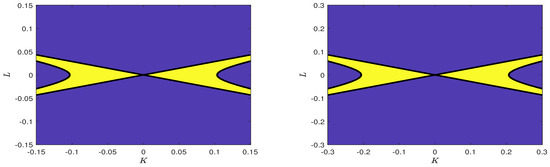
Figure 1.
Modulation instability bands in the plane from (20) for a finite depth case, , s for a 5 s carrier wave; m (left) and m (right). Solid lines are the boundaries of modulation instability regions. Light yellow areas correspond to .
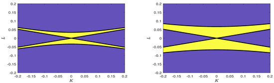
Figure 2.
Modulation instability bands on the plane from (20) for a shallow water case , s for a 5 s carrier wave; m (left) and m (right). Solid lines are the boundaries of modulation instability regions. Light yellow areas correspond to .
4. Numerical Results
Modulation instability in the one-dimensional NLS X setting occurs when with wavenumber K such that , see (20) and the following discussion. For M of order m, K can be quite small, requiring a large domain to resolve the instability, if present. Hence, for numerical reasons, we rescale (4) and (5) as follows
Here, ∓ refers to and , respectively. Note that the units for t remain as “” which we refer to as “s”, as mostly we put .
- A second order Fourier split step method is applied to solve these systems (21)–(24). More details are described in Appendix A.
Note that there is no explicit dependence on the X-dispersion parameter in (25), but it will reappear in the transform from to X. Likewise, the dependence on is through the transformed amplitude . Similarl, y the line soliton (17) becomes
- In (29), the modulation wavenumbers in the transformed space are in directions, respectively.
4.1. Deep-Water Limit
In the deep-water limit, , and the Benney–Roskes system (4) and (5) reduces to the forced two-dimensional nonlinear Schrödinger Equation (12). From (21), the rescaled form is
- We will present the results using the dimensional amplitude . For a 5 s wave, s. From the linear dispersion relation m setting m s. Then, from (14) we conclude that m s, m s and m.
4.1.1. Case 1: Peregrine Breather
The simulations were performed in the rescaled Equation (30) with the initial condition (25) at . When s and m, the Peregrine breather in one dimension along the axis is given by (25). The initial condition is at s with (M = 0.392, 1.959 m). The simulations for were over the time period s with time step s. The simulations for were over the time period s, a shorter time since small waves propagated to the boundaries as time increased. The computational domain is with the number of Fourier modes for each spatial direction. Since this case has an exact solution in the form of a one-dimensional Peregrine breather, the accuracy of numerical solutions can be checked by measuring the root mean square error. It is found that it lies within the order of at each time step. Then, we will apply this resolution setting to simulate the other cases.
We solve numerically (30) for B but plot the solution for A. Surface plots of when s and m for are shown in Figure 3 and Figure 4, respectively. Initially a Peregrine breather forms as s. Then for s, the wave amplitude decreases and disperses along the direction due to modulation instability on the background, as expected. In these cases, no Y dependence is discernible. In Figure 3, at , the background amplitude is m, and the peak amplitude is m, which is three times that of the initial background. The time scale for the evolution of these modulation instability oscillations is of order . The oscillations are just discernible for and become overwhelming for , where at s secondary peaks are emerging.
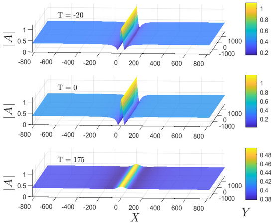
Figure 3.
Deep-water limit: Case 1, surface plot of from 2DfNLS (12) when , s and m.
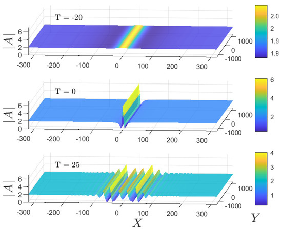
Figure 4.
Deep-water limit: Case 1, s and m, surface plot of from 2DfNLS (12) when .
Cases with Y dependent effects in (15) through the envelope are examined with m. The results for and are shown by contour plots in Figure 5 and Figure 6. For the smaller value of wave amplitude , modulation instability now occurs clearly in both the X and Y directions. Transverse modulation instability through is demonstrated as two sideband waves appear symmetrically on each side of the initial wave. These grow at the expense of the main wave and become dominant when the initial wave has decayed. These effects appear more in the Y than in the X direction.
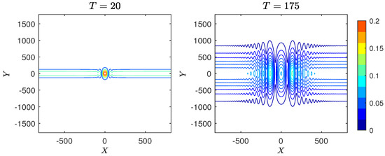
Figure 5.
Deep-water limit: Case 1, s and m, contour plot of from 2DfNLS (12) when .
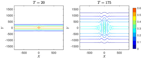
Figure 6.
Deep-water limit: Case 1, s and m, contour plot of from 2DfNLS (12) when .
For the larger value of wave amplitude , the wave has split into smaller amplitude waves along the X direction as for the case m and then disperses in both directions, more so in the Y than in the X direction. The energy (10) is preserved constantly when s indicating the accuracy of the numerical scheme.
When wind forcing is added, we consider three values of , s. The initial condition is again a Peregrine breather (25) with two values for the amplitude, and with m as considered above. We show contour plots when s and m as representative cases. Contour plots when are shown in Figure 7. As time increases, large waves develop, first narrow in the X direction and then dispersing in both directions. Large variation appears in the Y direction. A series of Peregrine breathers develop along the X direction. A case with a larger initial amplitude provides larger wave growth and more chaotic behaviour.
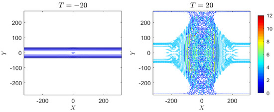
Figure 7.
Deep-water limit: Case 1, s and m, contour plot of from 2DfNLS (12) when .
Modulation instability occurs on a time scale of order of clearly seen in this 2DfNLS model. The predicted energy growth rate and the results from the 2DfNLS are shown in Figure 8 (left). Note that for the Peregrine breather (15), the energy E scales as , modulo slowly varying functions of T, and so the amplitude grows as , twice the linear value. Plots of the maximum of are shown in Figure 8 (right). The maximum wave amplitude decays monotonically due to dispersion when s, but it grows exponentially when s from the forcing effect.
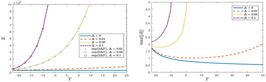
Figure 8.
Deep-water limit: Case 1, plots of E from (10) and the maximum of for for various values of .
4.1.2. Case 2: Line Soliton
The initial condition is (27) with envelop support m. We solve for B in the rescaled form (21) and consider two cases with , ( m) similar to the previous case. Here, we show the result for as representative since it has similar features to a case with smaller initial amplitude, but this case with a larger shows more effects. We set and m s, then and .
This case with is shown in Figure 9. Without forcing, s, the envelop soliton disperses over a long time due to the Y-dependent envelop. The centre of the envelop wave moves in the X direction with a constant speed V.
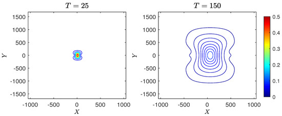
Figure 9.
Deep-water limit: Case 2, s and m, contour plot of from 2DfNLS (12) when .
A representative case with forcing is shown in Figure 10 with s. The wave amplitude grows in time with the generation of large amplitude breathers and solitons initially moving in the X direction. These become chaotically distributed throughout the domain at longer times.
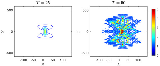
Figure 10.
Deep-water limit: Case 2, s and m, contour plot of from 2DfNLS (12) when .
The variation of energy over time is shown in Figure 11 (left). The growth rate of the wave amplitude again agrees with the predicted growth rate for this type of initial condition. The maximum of the wave amplitude over time is shown in Figure 11 (right). For small forcing coefficient, s, the initial wave amplitude decreases due to dispersion, but with sufficiently large forcing, s, the maximum amplitude wave in the domain is excited. The maximum amplitude grows in time but not monotonically due to the generation of breathers and solitons.
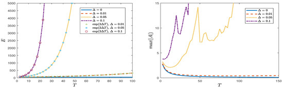
Figure 11.
Deep-water limit: Case 2, plots of E from (10) and the maximum of for for various values of .
4.1.3. Case 3: Long Wave Perturbation
The initial condition is (28) at s with equal envelope support m in the directions. We consider two cases with , ( m) and show the results only for since it shows the effects more clearly at earlier times.
In the absence of forcing, s, contour plots of when are shown in Figure 12. The initial amplitude generates two large breathers along the X direction that can be seen at s. This then disperses smoothly in both directions with a larger dispersion in the Y direction as seen at s.
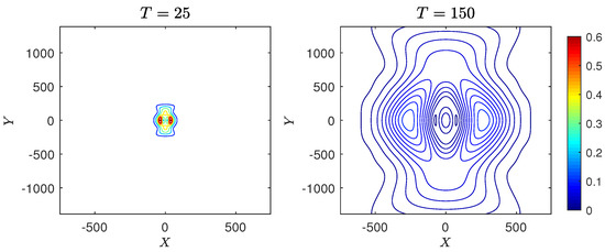
Figure 12.
Deep-water limit: Case 3, s and m, contour plot of from 2DfNLS (12) when .
When there is forcing, s, contour plots of when and s are shown in Figure 13. At early times s, many wave peaks develop around the centre of the initial amplitude, and modulation is dominant in the Y direction. Forcing enhances these waves and their interactions which become chaotic at later times, s. with the larger variation again in the Y direction, and many wave peaks appear along the Y direction. This greater variation in the Y direction than in the X direction is consistent with the linear modulation stability analysis, see for instance Grimshaw [34].
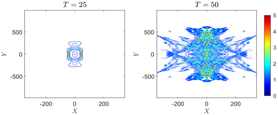
Figure 13.
Deep-water limit: Case 3, s and m, contour plot of from 2DfNLS (12) when .
Plots of the maximum amplitude shown in Figure 14 (right) reveal different growing amplitudes, a new feature with this type of initial condition. The initial wave has only a small growth at early times, s for all s. This is due to modulation instability for this type of initial condition. When s, forcing affects wave growth which becomes increasingly oscillatory, indicating the dominance of forcing over modulation instability in terms of wave growth.
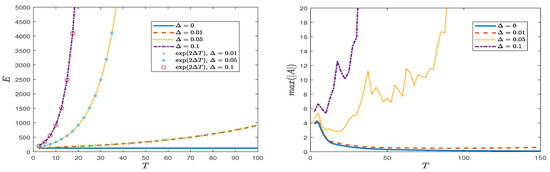
Figure 14.
Deep-water limit: Case 3, plots of E from (10) and the maximum of for for various values of .
The predicted growth rate of E still gives a good prediction as can be seen in Figure 14 (left). When we consider the relationship between and E, the growth rate is exponentially increasing, while does not but differs depending on the magnitude of . There is a threshold of such that the modulation of the wave amplitude will increase or decrease after the modulation stage, around s in our simulations. An explicit expression for this behaviour remains challenging. A physical interpretation of the modulation of these small amplitude waves could be as a source of rogue waves since rogue waves can arise due to modulation instability, and we note that in Figure 14 (right), the maximum of is greater than many times from that of the previous stage.
4.1.4. Case 4: Periodic Perturbation
Modulation instability of a periodic plane wave is described in Section 3, case 4, see (20) and the following text. Modulation instability occurs in a band in the plane, similar to that shown for finite depth in Figure 1. We set in (29) for all cases of simulations in this case 4, including cases of finite depth and the shallow water case described below. Using the flow parameters for deep water described above for a 5 s carrier wave, the instability band in the plane emerges from the K-axis for m. For m, the instability is barely discernible but can be seen when m.
For this deep water case, in the absence of forcing, s, we simulate two cases of L, m and m. The first case is to investigate the modulation instability band m when , so we set , m, m and m. After running for s, the modulation of a periodic plane waves is stable with a constant maximum amplitude. Next, we describe an unstable case with a smaller . The contour plots of when , m and m are shown in Figure 15. After running the simulations for s, the modulation of the periodic plane waves is unstable with increasing and steepening of the wave amplitude. Some waves appear at the troughs of the periodic plane wave. These results show modulation instability when is decreased in the unstable band as expected. Contour plots of when , m, m and m are shown in Figure 16. After running for s, the modulation of the periodic plane wave is unstable with the maximum amplitude increasing as time increases. High frequency waves develop chaotically over the entire domain. These simulations for and when m agree with the theoretical result of a modulation instability band m in deep water. A larger initial M results in more modulation instability in this case of s.
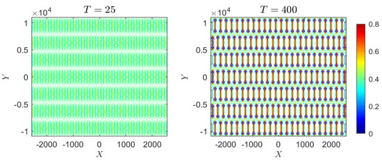
Figure 15.
Deep-water limit: Case 4, s and , contour plot of from 2DfNLS (12) when , m and m.
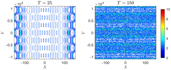
Figure 16.
Deep-water limit: Case 4, s and , contour plot of from 2DfNLS (12) when , m and m.
Then, to investigate two-dimensional effects, we set m and m for initial , m and simulate for s. The modulation of a periodic plane wave when m is stable, and we can now see modulation effects in both spatial directions with the maximum amplitude maintained, see the maximum amplitude in Figure 17 (right) when . In this case, when is small, the instability region is also small. The periodic plane wave is expected to be modulation unstable for large L and M. Contour plots when increases to , m for m and m are shown in Figure 18; modulation instability occurs with increasing amplitude over s.
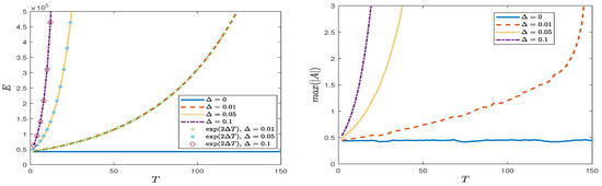
Figure 17.
Deep-water limit: Case 4, plots of E from (10) and the maximum of for , m and m for various values of .
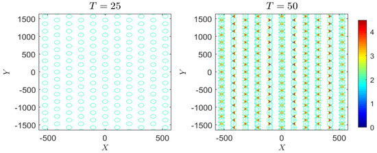
Figure 18.
Deep-water limit: Case 4, s and , contour plot of from 2DfNLS (12) when , m and m.
To study forcing, we put the forcing s and the initial , m for m and m where this previous unforced case shows modulation instability with the maximum amplitude maintained. When forcing is included, the maximum amplitude increases over time, see Figure 17 (right). The energy also increases and agrees with the theoretical growth rate, see Figure 17 (left).
4.2. Finite Depth
When and is finite, there is modulation instability in the direction, as , with , wavenumbers as in (20), see Grimshaw [34], Benney and Roskes [42]. In our simulations, we set and again consider a 5 s carrier wave, so that , s . Then, the wavenumber m and the water depth m. The wave phase speed m s and from (3), m s. Then from (6)–(9), the coefficients are and m s. We will solve for B in (21) where and . Compared to the deep water case in Section 4.1, has decreased from m s to m s, has increased marginally from m s to m s, and has decreased from m to m. The nonlocal nonlinear term Q is expected to have the same sign as that is positive and the opposite sign to . The implication is that compared to the deep water case, nonlinear effects are reduced and take longer to be seen, while the modulation scale in the X direction is decreased, with little change to that in the Y direction.
4.2.1. Case 1: Peregrine Breather
The simulations were performed in the rescaled Equation (21) and plotted using A in coordinates. The initial condition is (25) at s with m, and m). The computational domain is with the number of Fourier modes for each spatial direction.
In the absence of forcing, s, contour plots at various times for the case are shown in Figure 19. The results are similar to the deep water case for the same value of which is small as shown in Figure 5. Modulation instability occurs as the wave amplitude decreases and then disperses in both directions as time increases. Large dispersion occurs in the Y direction that can be seen at s. The case of is shown in Figure 20. This case shows a different pattern. Modulation instability occurs that can be seen at . The wave amplitude does not decay smoothly but with modulation and a high frequency of oscillations from many small waves. This feature of an unforced case can be seen clearly in terms of the maximum of amplitude against time in Figure 21. The value of the initial amplitude directly affects the modulation instability at long times. Note that there are some differences from the deep water case in Figure 8 when and s.
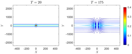
Figure 19.
Finite depth: Case 1, , s and m, contour plots of when .
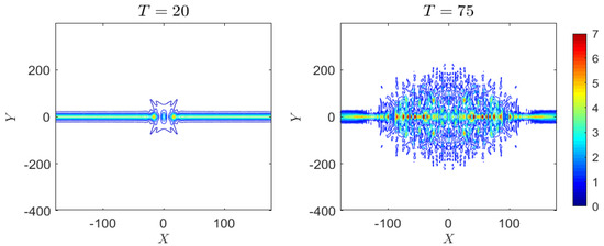
Figure 20.
Finite depth: Case 1, , s and m, contour plots of when .
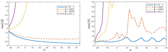
Figure 21.
Finite depth: Case 1, plots of the maximum of for (left) and (right) for various values of .
When forcing is added, we set s. A representative case when and s is shown in Figure 22. The simulations were performed over a short time period ( s) since the initial wave grows rapidly due to the forcing effect. It can be seen at that the Peregrine breather with a forcing effect will develop large waves near the centre area at s, and small waves disperse mainly in the Y direction.
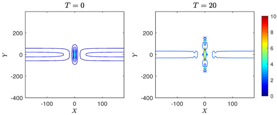
Figure 22.
Finite depth: Case 1, , s and m, contour plots of when .
While the forcing interacts with the modulation of the Peregrine breather, the energy conservation from (10) remains preserved. The energy plots of numerical simulations for various values of are shown in Figure 23 which grows as . Although the energy follows the theoretical prediction, the numerical solutions, especially when s and s, may not have physical meaning since many large waves have developed chaotically throughout the domain. The maximum of the wave amplitudes is greater than the water depth of m which is not realistic for these small amplitude models.
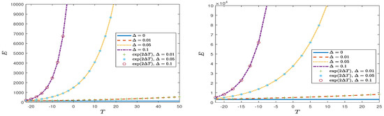
Figure 23.
Finite depth: Case 1, plots of E from (10) for (left) and (right) for various values of .
4.2.2. Case 2: Line Soliton
The initial condition is (27) with envelop support m. We solve for B in the rescaled Equation (21) and consider two cases of , ( m) and will show only the case of . All flow parameters are calculated by the same formulae with m s as done in the deep water case.
The results when without forcing are shown in Figure 24. The initial envelop soliton is moving in the X direction with dispersion similar to the deep water case, but here there is more dispersion effects in the X direction along .
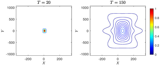
Figure 24.
Finite depth: Case 2, , s and m, contour plots of when .
The results for a forcing case, s, when are shown in Figure 25. Many breathers grow over time as seen at s and become chaotically distributed throughout the domain in a short time. Large variations appear in the Y direction, while many excited large waves are moving in the X direction.
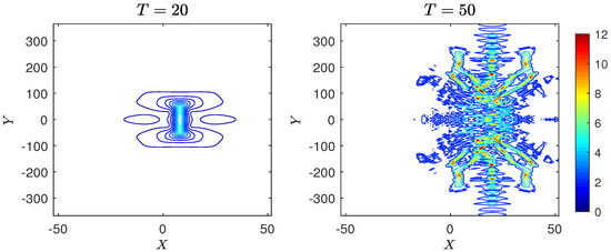
Figure 25.
Finite depth: Case 2, , s and m, contour plots of when .
The conservation of energy E is preserved when s. and E grows with the growth rate as shown in Figure 26 (left). The maximum amplitudes over time when for various values of are shown in Figure 26 (right). The behaviour is similar to the deep water case in that the maximum amplitude increases in an oscillatory manner after a particular time when due to modulation instability.
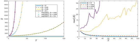
Figure 26.
Finite depth: Case 2, , plots of E from (10) and the maximum of for for various values of .
4.2.3. Case 3: Long Wave Perturbation
As in the deep water case in Section 4.1.3, we set m. In the absence of forcing, contour plots of when m) are shown in Figure 27. This initial amplitude produces many breathers and their interactions, see s. When comparing with Figure 12 for the corresponding deep water case, many breathers in this finite depth case are generated, more than in the deep water case, and these are dense with a smaller support area. These then disperse at the longer time, see s.
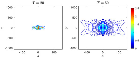
Figure 27.
Finite depth: Case 3, , s and m, contour plot of when .
When there is forcing, contour plots of when and s are shown in Figure 28. The forcing enhances the breather interactions which become chaotic at later times. Many peaks are distributed throughout the domain in both the X and Y directions.
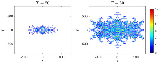
Figure 28.
Finite depth: Case 3, , s and m, contour plot of when .
Plots of the maximum amplitude shown in Figure 29 (right) reveal different growing amplitudes for each forcing value. There is a modulation stage around s. After this stage, forcing still affects the wave growth that increases in an oscillatory manner, similar to the deep water case. The predicted growth rates of E still give good predictions as can be seen in Figure 29 (left). Overall, the energy law is preserved with exponential growth rate for all values of .
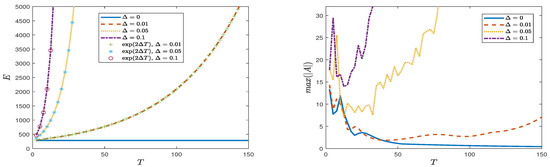
Figure 29.
Finite depth: Case 3, , plots of E from (10) and the maximum of for for various values of .
4.2.4. Case 4: Periodic Perturbation
Modulation instability of a periodic plane wave solution is described by (20) and the following text. Using the flow parameters for a finite depth described above for a 5 s carrier wave, the modulation instability region in the plane when m and m are shown in Figure 1 (left) and (right), respectively. Modulation instability occurs in the region around the K axis for this depth. There is an instability band in the plane emerging from the K-axis for m.
In the absence of forcing s, two cases of and are investigated. Contour plots of when , m for m and m are shown in Figure 30. After running for s, the modulation of periodic plane waves is unstable with increasing maximum amplitude; this case can be compared with the deep water case in Figure 15. A case of , m with m and m is also investigated. Modulation instability occurs with the maintained maximum amplitude over s. When is increased to , m contour plots of are shown in Figure 31. The modulation of the periodic plane wave is unstable over s with the development of breathers. High frequency waves develop chaotically over the two-dimensional domain. A larger initial results in more modulation instability.
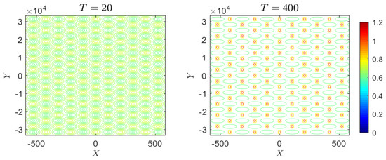
Figure 30.
Finite depth: Case 4, s, contour plot of when , m and m.
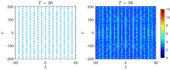
Figure 31.
Finite depth: Case 4, s, contour plot of when , m and m.
To study forcing, we put s with an initial , m with m and m. For small forcing s, periodic plane waves are modulated with amplitude increased, see Figure 32 at s. For larger forcing, the wave amplitude increases rapidly at early times. Forcing induces high frequency waves and waves growing throughout the domain. Plots of the maximum amplitude are shown in Figure 33 (right). The energy also increases and agrees with the theoretical growth rate, see Figure 33 (left).
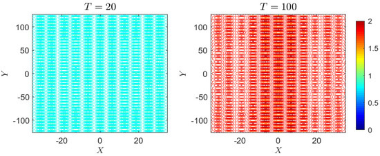
Figure 32.
Finite depth: Case 4, s, contour plot of when , m and m.
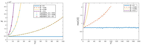
Figure 33.
Finite depth: Case 4, plots of E from (10) and the maximum of for , m and m for various values of .
4.3. Shallow Water
When , we set and again consider a 5 s carrier wave, so that , s, the wavenumber m and the water depth m. The wave phase speed m s and from (3), m s. Then, from (6)–(9), the coefficients are and s. We solve for B in (21) where , . Since now , both Peregrine breathers and line solitons are singular along the X axis. Nevertheless, we simulate them by ensuring that at the initial time the singularities lie outside the numerical -domain.
4.3.1. Case 1: Peregrine Breather
The Peregrine breather (25) using the sign corresponding to is singular at , where
- Hence at the initial time , we choose so that are outside the computational -domain. In the numerical simulations, the initial time is s with m and m). The singularities are at . To avoid these singularities, we set the computational domain with the number of Fourier modes for each spatial direction.
In the absence of forcing, s, contour plots at various times are shown in Figure 34. Modulation instability occurs mainly along the X direction emanating from the X boundaries as now expected, while the wave amplitude disperses in both directions as time increases. The outcome can be compared to the finite depth case for the same value of as shown in Figure 20. The shallow water case shows rapid modulation that can be seen at s in Figure 34. The wave amplitude does not decay smoothly but with modulation as can be seen in the maximum of in Figure 35 (right). The modulation occurs clearly at the early time step (around s), while the modulation occurs more slowly compared with the finite depth case in Figure 21 (right) (around s).
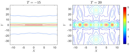
Figure 34.
Shallow water: Case 1, , s and m, contour plot of when .
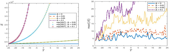
Figure 35.
Shallow water: Case 1, , plots of E from (10) and the maximum of for for various values of .
When forcing is added, we set s. The forcing affects the modulation of this singular Peregrine breather causing wave growth, but the energy (10) remains preserved. Energy plots for various values of are shown in Figure 35 (left) which grows as as expected. The maximum values of for various values of are shown in Figure 35 (right), and these grow with high modulation.
4.3.2. Case 2: Line Soliton
- This is singular at . At these are at and can be placed outside the computational -domain by appropriate choice of through . Here, we put ( m), and then the nearest singular points are . To avoid these singularities, we set the computational domain with the number of Fourier modes for each spatial direction. We simulate only over a short time period s to avoid some reflection effects from the truncated boundaries.
The results when and m without forcing is shown in Figure 36. The initial envelop soliton is moving in the X direction with modulation instability along the X axis, see s. During the motion of the modulated soliton, dispersion effects also appear as can be seen by the maximum of over time in Figure 37 (right).
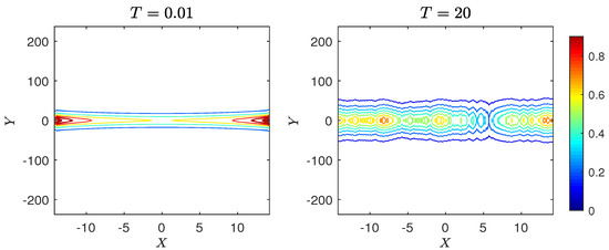
Figure 36.
Shallow water: Case 2, , s and m, contour plot of when .
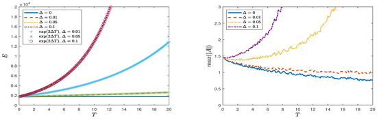
Figure 37.
Shallow water: Case 2, , plots of E from (10) and the maximum of for for various values of .
Conservation of energy E is preserved when s and grows with the growth rate as shown in Figure 37 (left). The maximum amplitudes over time when for various values of are shown Figure 37 (right). The maximum amplitude increases in an oscillatory manner when s due to modulation instability and forcing. Modulation instability is mainly along the X axis for this shallow water case.
4.3.3. Case 3: Long Wave Perturbation
The initial condition is (28) again with equal envelope support m in the directions. The simulations were performed in the rescaled Equations (21) and (22). The computational domain is with the number of Fourier modes for each spatial direction. We simulate two cases with ( m), but we show only the case as it is representative.
In the absence of forcing, s, contour plots of are shown in Figure 38. Many breathers occur at the initial stage, see s, which are modulated and disperse in both directions; the effect in the Y direction is faster than in the X direction. These patterns are similar to the finite depth case shown in Figure 27, but in this shallow water case there are many more smaller waves. For this initial amplitude ( m), the wave elevation of is over a water depth m, and so the small parameter must be chosen to ensure that m, placing an implicit limitation on the use of the asymptotic system (4) and (5) in shallow water. For instance when , we require that .
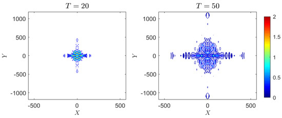
Figure 38.
Shallow water: Case 3, , s and m, contour plot of when .
The simulation was conducted only for a short time period since modulation appears rapidly in both directions. Interpretation as modulation instability agrees with the linear modulation stability analysis in two dimensions, see [17,34], although this is based on the perturbation wavenumber plane. The instability is baseband as it emerges from with progressively larger wavenumbers as time increases, see contour plots at s of Figure 38.
When there is forcing, contour plots of when and s are shown in Figure 39. Similar to the finite depth case, the forcing effect enhances the breathers interactions. Many peaks are generated sparsely throughout the domain.
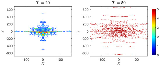
Figure 39.
Shallow water: Case 3, , s and m, contour plot of when .
Plots of E from (10) over time for and various values of are shown in Figure 40 (left). The simulation results again agree with the theoretical growth rate for this type of initial condition over the shallow water depth. The maximum value of over time is shown in Figure 40 (right). Unlike the deep water and finite depth cases, the maximum amplitude decreases relatively monotonically at the early stage in the unforced case. There is no sign of excitation in terms of the maximum amplitude. For forcing cases with s, the maximum of in shallow water grows more rapidly than in the finite depth case. For instance, at s the maximum of in Figure 29 is about m, while it is approximately 25–30 m in Figure 40. A similar argument can be made for the deep water when considering the maximum of in Figure 14 for s. However, now so the physical time scale here is increased as and is closer to the finite depth case.
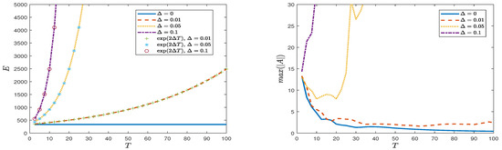
Figure 40.
Shallow water: Case 3, , plots of E from (10) and the maximum of for for various values of .
4.3.4. Case 4: Periodic Perturbation
Modulation instability of a periodic plane wave is described by (20) and the following text. Using the flow parameters of shallow water flow described above for a 5 s carrier wave, the modulation instability region in the plane when m and m are shown in Figure 2 (left) and (right), respectively. Modulation instability emerges from with a band along the L-axis, implying there is transverse modulation instability, see Peregrine [43].
In the absence of forcing, , we fix m and m to compare the results with the deep water and finite depth cases described above. Two cases of and are investigated. Contour plots of when , m are shown in Figure 41. After running for s, the modulation of a periodic plane wave is unstable with increasing maximum amplitude. This shows that this shallow water depth case enhances modulation instability. At a longer time s, large waves develop along the X axis with very high frequency along the Y axis, corresponding to the transverse modulation instability along the L-axis. Cases of smaller values m and m when m for , m were also investigated but are not shown here. The results show modulation instability with the development of large amplitude breathers. To compare the results with a case of smaller L, we set , m, m and m; the corresponding contour plots of are shown in Figure 42. Modulation instability occurs but slowly with a slight increasing of the maximum amplitude compared with Figure 15 and Figure 30 for other depths. Contour plots of when , m are shown in Figure 43. After running for s, the modulation of the periodic plane wave is unstable with increasing maximum amplitude as time increases. Instability occurs at an early time step, see at s where high frequency waves develop over the entire domain. A larger initial results in more modulation instability.
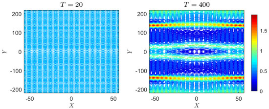
Figure 41.
Shallow water: Case 4, s, contour plot of when , m and m.
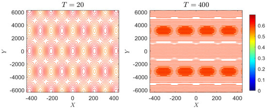
Figure 42.
Shallow water: Case 4, s, contour plot of when , m and m.
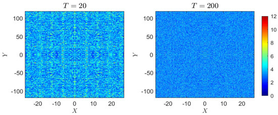
Figure 43.
Shallow water: Case 4, s, contour plot of when , m and m.
To investigate forcing, we set s with an initial , m for m and m. Again, forcing enhances high frequency waves growing throughout the domain. Plots of the maximum amplitude are shown in Figure 44 (right). The energy also increases and agrees with the theoretical growth rate, see (10).
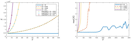
Figure 44.
Shallow water: Case 4, plots of E from (10) and the maximum of for , m and m for various values of .
5. Summary and Discussion
In the articles Maleewong and Grimshaw [23,24], we examined the evolution of water wave groups, with and without wind forcing, in a one horizontal space co-ordinate setting based on the one-dimensional forced nonlinear Schrödinger Equation (fNLS). In this paper, that study has been extended to two horizontal space co-ordinates using the forced Benney–Roskes system (4) and (5), which is a two-dimensional NLS-type equation with a nonlocal nonlinear term. As in Maleewong and Grimshaw [23,24], our approach is to use four contrasting initial conditions, each of which in an unforced one-dimensional (X) setting would lead to wave groups propagating in the X-direction.
Each initial condition case is explored numerically, and the results are described in detail in Section 4 in three scenarios, deep water (), finite depth () and shallow water (), where and each scenario is for a 5 s carrier wave. The initial conditions are described in Section 3. Case 1 is a Peregrine breather designed to produce a single Peregrine breather in the unforced NLS Equation. Case 2 is a line soliton designed to produce a single line soliton in the unforced NLS Equation. Case 3 is a long wave perturbation, which is expected to produce line solitons and Peregrine breathers in the unforced NLS Equation. In each of these three cases, the initial condition is augmented with a slowly varying Y-envelope (16). Case 4 is a periodic perturbation which demonstrates modulation stable and unstable outcomes in the unforced NLS Equation. Here, the periodic perturbation has both X and Y components with K and L wavenumbers, respectively.
Case 1 Peregrine breather: when s, see Figure 5 for deep water and m, modulation effects appear along the X direction with dispersive effects in the Y direction due to term . The result for finite depth in Figure 19 when m is similar to the deep water case. However, when m in finite depth, the results are different as shown in Figure 20. The modulation of large amplitude waves develop along the X direction with a chaotic nature in two dimensions. The effect of finite water depth can be seen more clearly in Figure 34 when the water depth is shallow. Large breathers develop along the X direction with modulation effects in the Y direction. When s, the energy E of all simulated water depths grows exponentially with the theoretical growth rate . The maximum of grows in time. A larger initial leads to an increase of in an oscillatory manner.
Case 2 Line soliton: when s, see Figure 9 for deep water, a line soliton moves with constant speed in the X direction, while the main feature is the dispersion effects in two dimensions. A finite depth case is shown in Figure 24 and shows dispersion effects similar to the deep water case. An adjustment is needed for the initial condition of a line soliton in shallow water since then and singularities appear in the domain. Hence, we truncate the computational domain so that the singularities are initially outside. The initial amplitude can only be set to be a small value, and we perform the simulation over a short time to avoid unexpected effects from the truncated boundaries. The line soliton is then along the X direction in shallow water as expected, but now there is a rapid modulation along the X axis, see Figure 36. When s, large amplitude waves develop in the two-dimensional domain along with the moving soliton. Some small waves are generated over the moving soliton as time increases. This is the main feature in both deep and finite depth cases. The grows oscillating in time while E is preserved and agrees with the theoretical growth rate.
Case 3 Long wave perturbation: when s, we can see the modulation of breathers at an early time. These then disperse in the Y direction more than in the X direction, see Figure 12 for a deep water case. This feature also occurs in finite depth, see Figure 27, but with more modulations. The modulation of breathers at an early time is dense for a shallow water case, see Figure 38. The modulation is enhanced, and large variations appear in the Y more than in the X direction. When s, grows oscillating in time, and many peaks over many small waves can be observed. The growth wave amplitude when forcing is inserted is sensitive to the water depth. When , finite depth and shallow water cases are more sensitive to forcing than for a deep water case. Small s can induce growth of maximum amplitude for finite depth and shallow water but not for deep water. In all three cases of water depth, E is preserved and agrees with the theoretical growth.
Case 4 Periodic perturbation: s modulation instability in the Benney–Roskes system (4) and (5) was analysed by Benney and Roskes [42] and extended to by Grimshaw [34]. It can also be deduced directly from the slant-wise forced NLS Equation (11). Modulation instability occurs when , see (20). For simplicity, when the initial periodic plane wave is considered in one dimension , there is modulation instability, as in the one-dimensional NLS Equation, when , . However, in two space dimensions modulation, instability occurs in bands of the plane, and now the value of the depth parameter characterises the instability region. In deep water and when in finite depth, the instability band emanates from the K axis, where . However, in shallow water when , the instability band emanates from the L-axis, where , see Benney and Roskes [42], Peregrine [43]. In this work, we have performed some numerical simulations to observe these theoretical results. In deep water and finite depth, we set m to represent the limit while setting M and K to satisfy the instability condition. A periodic plane wave is modulation unstable with wave amplitude increasing and steepening in time, see Figure 15 for deep water and Figure 30 for finite depth, although even in these cases the initial amplitudes are small: m for deep water and m for finite depth. When is set to be larger, m for deep water and m for finite depth, a periodic plane wave is unstable with high frequency waves developing chaotically over the entire domain. Two-dimensional effects were simulated by setting m and m. Then, the solutions of the deep water and finite depth cases were modulation stable when , since the instability region is now narrow. However, in shallow water, when m, the solution is modulation unstable, see Figure 41. These results show that the water depth affects the modulation stability of a periodic plane wave. In all three cases of water depth, the larger value of initial amplitude results in more modulation instability. Again when s, the conservation of energy E is preserved with the growth rate for this type of initial condition.
Overall, the results resemble those for the one-dimensional fNLS Equation described by Maleewong and Grimshaw [23,24], with the main difference that the additional Y spatial dimension allows for enhanced wave growth due to modulation instability with a Y component. This is especially notable in the shallow water scenario. However, unlike the one-dimensional case, there is a prevalence of breather formation over line soliton formation. This we attribute to the enhanced modulation instability when a Y dependence is allowed. In addition, we note that the Benney–Roskes system (4) is hyperbolic with respect to the highest derivatives, while (5) is elliptic, and the former would inhibit the phase relationship needed for line soliton formation.
The forced Benney–Roskes system (4) and (5) is an asymptotic reduction from a fully nonlinear air–water system. We plan to test the results obtained here using a modified Euler system with two horizontal space dimensions analogous to that with one horizontal space dimension described by Maleewong and Grimshaw [24]. A fully nonlinear air–water system with a turbulent wind is well beyond our computational capacity which is why we prefer the reduction to a modified Euler system which as described by Maleewong and Grimshaw [24] is a one-fluid (water) system with wind forcing modelled following Miles [2].
Author Contributions
Conceptualization, R.H.J.G.; Methodology, M.M. and R.H.J.G.; Formal analysis, R.H.J.G.; Investigation, M.M.; Data curation, M.M.; Writing—original draft, M.M. and R.H.J.G. All authors have read and agreed to the published version of the manuscript.
Funding
This research received no external funding.
Data Availability Statement
The data presented in this study are available on request from the corresponding author.
Conflicts of Interest
The authors declare no conflict of interest.
Appendix A. Numerical Method
We describe the Fourier split step method to solve the forced Benney–Roskes system (4)–(5) numerically. Assume that and Q can be written in terms of Fourier series in two dimensions as follows.
and
where and are the double Fourier transform of and Q, respectively, and and are the Fourier frequencies in the X and Y directions, respectively.
Applying the double Fourier transform in space dimensions X and Y to (5) yields,
for any j and k such that , then
- By taking the inverse Fourier transform, we can find when is known. At the initial time , is given. Then, we will know explicitly.
To calculate the numerical solution in time, we apply the second-order Fourier split step method. First, rewriting (4) as
- Next, we split the operators by writingwhere the linear and nonlinear operators, and , are defined by
- Define the notationsandwhere refers to time at step m with time spacing . Calculating the numerical solution in time is composed of three steps as follows.where E is . Then, for a given initial condition , we use (A1) to approximate Q and then calculate A using (A2) for the next time step. Directly, we can approximate B in the rescale coordinate from (21) using the transformations (23) and (24).
References
- Grimshaw, R.; Hunt, J.; Johnson, E. IUTAM Symposium Wind Waves, 2017; Elsevier IUTAM Procedia Series; Elsevier: Amsterdam, The Netherlands, 2018; Volume 26, pp. 1–226. [Google Scholar]
- Miles, J.W. On the generation of surface waves by shear flows. J. Fluid Mech. 1957, 3, 185–204. [Google Scholar] [CrossRef]
- Janssen, P. The Interaction of Ocean Waves and Wind; Cambridge University Press: Cambridge, UK, 2004. [Google Scholar]
- Cavaleri, L.; Alves, J.H.; Ardhuin, F.; Babanin, A.; Banner, M.; Belibassakis, K.; Benoit, M.; Donelan, M.; Groeneweg, J.; Herbers, T.; et al. Wave modelling: The state of the art. Prog. Oceanogr. 2007, 75, 603–674. [Google Scholar] [CrossRef]
- Phillips, O.M. On the generation of waves by turbulent wind. J. Fluid Mech. 1957, 2, 417–445. [Google Scholar] [CrossRef]
- Phillips, O.M. Wave interactions - the evolution of an idea. J. Fluid Mech. 1981, 106, 215–227. [Google Scholar] [CrossRef]
- Jeffreys, H. On the formation of water waves by wind. Proc. R. Soc. A 1925, 107, 189–206. [Google Scholar]
- Belcher, S.E.; Hunt, J.C.R. Turbulent flow over hills and waves. Ann. Rev. Fluid Mech. 1998, 30, 507–538. [Google Scholar] [CrossRef]
- Wu, J.; Popinet, S.; Deike, L. Revisiting wind wave growth with fully coupled direct numerical simulations. J. Fluid Mech. 2022, 951, A18. [Google Scholar] [CrossRef]
- Sajjadi, S.G.; Drullion, F.; Hunt, J.C.R. Computational turbulent shear flows over growing and nongrowing wave groups. In IUTAM Symposium Wind Waves; Grimshaw, R., Hunt, J., Johnson, E., Eds.; Elsevier IUTAM Procedia Series; Elsevier: Amsterdam, The Netherlands, 2018; Volume 26, pp. 145–152. [Google Scholar]
- Sullivan, P.P.; Banner, M.L.; Morison, R.; Peirson, W.L. Impacts of wave age on turbulent flow and drag of steep waves. In IUTAM Symposium Wind Waves; Grimshaw, R., Hunt, J., Johnson, E., Eds.; Elsevier IUTAM Procedia Series; Elsevier: Amsterdam, The Netherlands, 2018; Volume 26, pp. 184–193. [Google Scholar]
- Wang, J.; Yan, S.; Ma, Q. Deterministic numerical modelling of three-dimensional rogue waves on large scale with presence of wind. In IUTAM Symposium Wind Waves; Grimshaw, R., Hunt, J., Johnson, E., Eds.; Elsevier IUTAM Procedia Series; Elsevier: Amsterdam, The Netherlands, 2018; Volume 26, pp. 214–226. [Google Scholar]
- Hao, X.; Cao, T.; Yang, Z.; Li, T.; Shen, L. Simulation-based study of wind-wave interaction. In IUTAM Symposium Wind Waves; Grimshaw, R., Hunt, J., Johnson, E., Eds.; Elsevier IUTAM Procedia Series; Elsevier: Amsterdam, The Netherlands, 2018; Volume 26, pp. 162–173. [Google Scholar]
- Zakharov, V.; Badulin, S.; Hwang, P.; Caulliez, G. Universality of sea wave growth and its physical roots. J. Fluid Mech 2015, 780, 503–535. [Google Scholar] [CrossRef]
- Zakharov, V.; Resio, D.; Pushkarev, A. Balanced source terms for wave generation within the Hasselmann equation. Nonlinear Process. Geophys. 2017, 24, 581–597. [Google Scholar] [CrossRef]
- Zakharov, V. Analytic theory of a wind-driven sea. In IUTAM Symposium Wind Waves; Grimshaw, R., Hunt, J., Johnson, E., Eds.; Elsevier IUTAM Procedia Series; Elsevier: Amsterdam, The Netherlands, 2018; Volume 26, pp. 43–58. [Google Scholar]
- Benney, D.J.; Newell, A.C. The propagation of nonlinear wave envelopes. J. Math. Phys. 1967, 46, 133–139. [Google Scholar] [CrossRef]
- Zakharov, V.E. The instability of waves in nonlinear dispersive media. Sov. Phys. JETP 1967, 24, 740–744. [Google Scholar]
- Zakharov, V.E. Stability of periodic waves of finite amplitude on the surface of a deep fluid. J. Appl. Mech. Tech. Phys. 1968, 9, 190–194. [Google Scholar] [CrossRef]
- Zakharov, V.E.; Ostrovsky , L.A. Modulation instability: The beginning. Physica D 2009, 238, 540–548. [Google Scholar]
- Grimshaw, R. Envelope solitary waves. In Solitary Waves in Fluids: Advances in Fluid Mechanics; Grimshaw, R., Ed.; WIT Press: Southampton, UK, 2007; Volume 45, pp. 159–179. [Google Scholar]
- Osborne, A.R. Nonlinear Ocean Waves and the Inverse Scattering Transform; Elseveier: Amsterdam, The Netherlands, 2010. [Google Scholar]
- Maleewong, M.; Grimshaw, R. Amplification of wave groups in the forced nonlinear Schrödinger equation. Fluids 2022, 7, 233. [Google Scholar] [CrossRef]
- Maleewong, M.; Grimshaw, R. Evolution of water wave groups with wind action. J. Fluid Mech. 2022, 947, A35. [Google Scholar] [CrossRef]
- Leblanc, S. Amplification of nonlinear surface waves by wind. Phys. Fluids 2007, 19, 101705. [Google Scholar] [CrossRef]
- Touboul, J.; Kharif, C.; Pelinovsky, E.; Giovanangeli, J.P. On the interaction of wind and steep gravity wave groups using Miles’ and Jeffreys’ mechanisms. Nonlin. Proc. Geophys. 2008, 15, 1023–1031. [Google Scholar] [CrossRef]
- Kharif, C.; Kraenkel, R.A.; Manna, M.A.; Thomas, R. The modulational instability in deep water under the action of wind and dissipation. J. Fluid Mech. 2010, 664, 138–149. [Google Scholar] [CrossRef]
- Onorato, M.; Proment, D. Approximate rogue wave solutions of the forced and damped nonlinear Schrödinger equation for water waves. Phys. Lett. A 2012, 376, 3057–3059. [Google Scholar] [CrossRef]
- Montalvo, P.; Kraenkel, R.; Manna, M.A.; Kharif, C. Wind-wave amplification mechanisms: Possible models for steep wave events in finite depth. Nat. Hazards Earth Syst. Sci. 2013, 13, 2805–2813. [Google Scholar] [CrossRef]
- Brunetti, M.; Marchiando, N.; Berti, N.; Kasparian, J. Nonlinear fast growth of water waves under wind forcing. Phys. Lett. A 2014, 378, 1025–1030. [Google Scholar] [CrossRef]
- Slunyaev, A.; Sergeeva, A.; Pelinovsky, E. Wave amplification in the framework of forced nonlinear Schrödinger equation: The rogue wave context. Physica D 2015, 301, 18–27. [Google Scholar] [CrossRef]
- Grimshaw, R. Generation of wave groups. In IUTAM Symposium Wind Waves; Grimshaw, R., Hunt, J., Johnson, E., Eds.; Elsevier IUTAM Procedia Series; Elsevier: Amsterdam, The Netherlands, 2018; Volume 26, pp. 92–101. [Google Scholar]
- Grimshaw, R. Generation of wave groups by shear layer instability. Fluids 2019, 4, 39. [Google Scholar] [CrossRef]
- Grimshaw, R. Two-dimensional modulation instability of wind waves. J. Ocean Eng. Mar. Energy 2019, 5, 413–417. [Google Scholar] [CrossRef]
- Segur, H.; Henderson, D.; Carter, J.; Hammack, J.; Li, C.M.; Pheiff, D.; Socha, K. Stabilizing the Benjamin-Feir instability. J. Fluid Mech. 2005, 539, 229–271. [Google Scholar] [CrossRef]
- Galchenko, A.; Babanin, A.; Chalikov, D.; Young, I.; Haus, B. Influence of wind forcing on modulation and breaking of one-dimensional deep-water wave groups. J. Phy. Ocean. 2012, 42, 928–939. [Google Scholar] [CrossRef]
- Rajan, G.; Bayram, S.; Henderson, D. Periodic envelopes of waves over non-uniform depth. Phys. Fluids 2016, 28, 042106. [Google Scholar] [CrossRef]
- Benilov, E.; Flanagan, J.; Howlin, C. Evolution of packets of surface gravity waves over smooth topography. J. Fluid Mech. 2005, 533, 171–181. [Google Scholar] [CrossRef]
- Benilov, E.; Howlin, C. Evolution of packets of surface gravity waves over strong smooth topography. Stud. Appl. Math. 2006, 116, 289–301. [Google Scholar] [CrossRef]
- Rajan, G.; Henderson, D. The linear stability of a wave train propagating on water of variable depth. Siam J. Appl. Math. 2016, 76, 2030–2041. [Google Scholar] [CrossRef]
- Helal, M.; Seadawy, A. Benjamin-Feir instability in nonlinear dispersive waves. Comput. Math. Appl. 2012, 64, 3557–3568. [Google Scholar] [CrossRef]
- Benney, D.J.; Roskes, G.J. Wave instabilities. Stud. Appl. Math 1969, 48, 377–385. [Google Scholar] [CrossRef]
- Peregrine, D.H. Water waves, nonlinear Schrödinger equations, and their solutions. J. Aust. Math. Soc. Ser. B 1983, 25, 16–43. [Google Scholar] [CrossRef]
- Mei, C.C. The Applied Dynamics of Ocean Surface Waves; Wiley-Interscience: Hoboken, NJ, USA, 1983. [Google Scholar]
- Chabchoub, A.; Grimshaw, R. The hydrodynamic nonlinear Schödinger equation: Space and time. Fluids 2016, 1, 23. [Google Scholar] [CrossRef]


Disclaimer/Publisher’s Note: The statements, opinions and data contained in all publications are solely those of the individual author(s) and contributor(s) and not of MDPI and/or the editor(s). MDPI and/or the editor(s) disclaim responsibility for any injury to people or property resulting from any ideas, methods, instructions or products referred to in the content. |
© 2023 by the authors. Licensee MDPI, Basel, Switzerland. This article is an open access article distributed under the terms and conditions of the Creative Commons Attribution (CC BY) license (https://creativecommons.org/licenses/by/4.0/).