Article

Transporting Particles with Vortex Rings

1
School of Physics and Engineering, ITMO University, 197101 St. Petersburg, Russia
2
Abrikosov Center for Theoretical Physics, Moscow Institute of Physics and Technology, 141701 Dolgoprudnyi, Russia
*
Author to whom correspondence should be addressed.
Fluids 2023, 8(12), 315; https://doi.org/10.3390/fluids8120315
Submission received: 10 October 2023 / Revised: 26 November 2023 / Accepted: 4 December 2023 / Published: 5 December 2023
(This article belongs to the Special Issue Vortical Flows in Memory of Professor Ippolit Stepanovich Gromeka)

Abstract

:
Due to their long-lived nature, vortex rings are highly promising for the non-contact transportation of colloidal microparticles. However, because of the high complexity of the structures, their description using rigorous, closed-form mathematical expressions is challenging, particularly in the presence of strongly inhomogeneous colloidal suspensions. In this work, we comprehensively study this phenomenon, placing special emphasis on a quantitative description of the ability of vortex rings to move the particles suspended in a liquid over distances significantly exceeding the ring’s dimensions. Moreover, within the study, we present straightforward analytical approximations extracted by using the fitting of the experimental and numerical simulation observations that reveal the dynamics of vortex rings transporting the microparticles. It includes both the dependence of the concentration on the distance traveled by the vortex ring and coefficients describing the evolution of vortex ring shape in time, which were not presented in the literature before. It turns out that despite the fact that 2D modeling is a simplification of the full 3D problem solution and is unable to capture some of the minor effects of real behavior, it has demonstrated a good consistency with the results obtained via experiments regarding the process of particles transportation.

1. Introduction

Hydrodynamics of turbulent flows has been in the spotlight of research for many decades. In particular, one of the most interesting phenomena studied to date is a toroidal vortex, also known as a vortex ring [1,2]. A vortex ring is a torus-shaped pattern of circulating fluid in which the liquid mostly revolves around an imaginary axis, forming a circular loop.
Theoretical and experimental investigations of these vortices [3,4], laws of their motion and mass exchange [5,6], and their capability to transport various objects created a number of important applications. Recent research in the field of computer modeling of turbulent flows and optimization methods for the simulation of various hydrodynamic effects [7] has made it possible to study complex processes that are difficult to describe analytically. The mentioned computer experiments allowed one to solve different engineering problems, such as, for example, a Lagrangian description of buoyancy effects on aircraft wake vorticity [8]. Another example of the engineering application of vorticity research is advancement the of helicopter technologies [9] by finding optimal ways to prevent helicopters from entering a dangerous vortex ring state. Moreover, the vortex rings can be used for extinguishing gas–oil well fires [10]—a device releasing a vortex ring of extinguishing agent is placed at the base of a burning gas fountain. There is another, quite different area of application—the formation of ring-shaped particles [11].
In this regard, it is quite clear that this phenomenon, which has such a wide range of applications, requires a comprehensive investigation. One of the key characteristics of toroidal vortices is their geometrical stability. As the vortex preserves its shape in time, the rings are capable of carrying and delivering microparticles over distances much larger than their size. Therefore, these rings can be used for the targeted delivery of various substances, which is attractive, for instance, for biomedical purposes [12]. Adding a pH indicator to a vortex allows a local determination of the acidity level in an environment [13]. In another example of targeted particle delivery, the controlled vortex rings reconnection is used, which changes the topology of the vortex ring, accompanied by repulsion in the plane perpendicular to the direction of propagation [14,15,16]. Several experimental studies focused on the flight distance of particles inside a vortex ring depending on the initial conditions [17,18,19,20,21,22,23,24], and theoretical estimates of the main vortex parameters were presented [25,26,27]. However, to the best of the authors’ knowledge, in the existing literature, neither the abilities of vortices to transport different microparticles nor the dependencies of the concentration of the particles in the vortex ring along the entire path of the movement have been studied numerically or analytically. In our work, we supplement our research with an empirical analysis including the development of simple analytical approximations and numerical ansatzes describing the dependence of the number of particles in a vortex ring on its characteristics. For this purpose, we perform rigorous simulations of vortex rings carrying small particles and corresponding experimental measurements with the subsequent usage of the obtained data to develop the mentioned approximations for the time evolution of velocity fields and particle concentration.
In the following sections, we describe the numerical model, velocity field approximation and its time evolution. For a more objective consideration of the movement of the vortex ring, it is necessary to use a 3D numerical model. It turns out that the experimental data obtained are in good agreement with the 2D simulations, and therefore, we address this simplification below. Also, an approximation for particle density is shown, and the particle loss mechanism is discussed together with a comparison to the obtained via the experimental setup data. The results of this study in the future can serve as the basis for studying the movement of particles suspended in liquids in toroidal turbulent flows with high Reynolds numbers.
The paper is organized as follows. In Section 2, we describe the numerical model and show the velocity field of vortex rings. In Section 3, velocity field approximation, its time evolution and an approximation for particle density in vortex ring are presented. The particle loss mechanism is also presented here for the physically interesting case. In Section 4, we show our experimental setup together with the obtained data. In Section 5, the data obtained are discussed and the experiment, numerically simulated and analytical results are compared. Section 6 contains the summary of the main results and concluding remarks.

2. Numerical Simulation

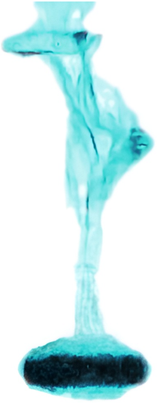
We simulated the system shown in Figure 1, consisting of a vortex ring and colloidal particles placed in it, via the Comsol Multiphysics software. A default segregated nonlinear iterative solver in COMSOL (FEM) with time stepping BDF with order 1–2 was used. The mesh size was up to 2.5 mm. Also, before, we solved the same problem using a 4 mm and 7 mm maximum mesh size to prove the accuracy. The CFD Module with a k- ω turbulence model [28] was chosen for numerical simulation. We chose this module due to the low Reynolds numbers in the vicinity of the vessel walls. To simulate particle motion in the water, we used the Schiller–Naumann with Mixture Model. The drag model of Schiller–Naumann is used to model the drag force between the particles and the fluid. By including inertia, Schiller–Naumann’s drag model extends Stoke’s expression for the stationary drag coefficient to flow regimes characterized by a higher Reynolds number. For a solid–liquid suspension with a high particle concentration at intermediate velocities, the Schiller–Naumann drag correlation shows good agreement [29,30]. For simplicity, we focus on the 2D simulations, which proved the ability to fit the experimental data quite well. We emphasize that the justification of this approach is associated only with good agreement with the experiment and the high difficulties associated with numerical calculations of numerous runs in the real three dimensions. Additionally, an argument in favor of this simplification is that the motion of liquid and particles around the vortex ring circle is much more intensive than the motion of the vortex ring around its axis. Here, we should note that we do not exclude that some additional effects may arise when the corresponding simulation is performed within the full 3D modeling. Apparently, it would give a more accurate understanding of the energy cascade processes in vortices, which are suppressed by local rotations, but the corresponding analysis should be the subject of a separate study.
To estimate the velocity field in vortex rings, we simulate the formation of these rings with an inlet boundary condition at the upper boundary of a tube (see Section 4 below). The membrane movement effect was modeled using the following spatial velocity distribution of the input flow: v i n l e t ( 1 | 2 x / d | ) , where v inlet 0.2 m/s, x is the radial distance from the tube center, and d is the tube diameter. The vorticity was estimated locally using the definition
ω = curl v .
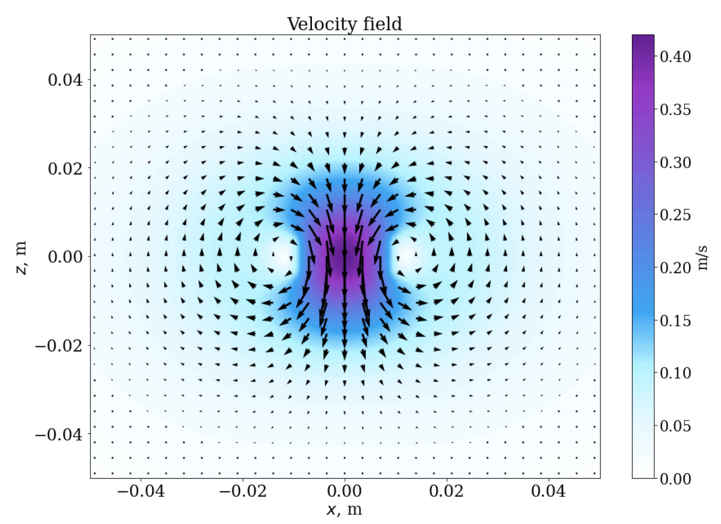
Furthermore, to analyze the particle distribution in the vortex rings, we modeled the formation of these rings using the velocity field distributions presented in the next section. At the initial moment, colloidal particles are placed within the central area of the vortex. The velocity field evolves with time, and the colloidal particles redistribute as the ring propagates. An example of the initial velocity field with an area containing the colloidal particles is shown in Figure 2.
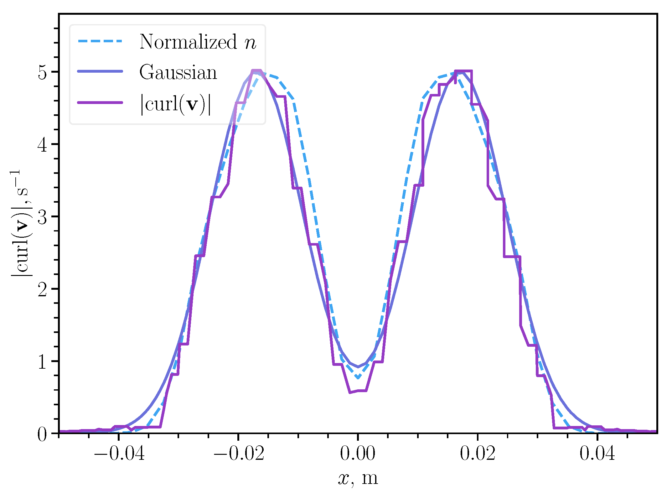
The results of our simulations are in good agreement with the existing basic theoretical results, which proves the validity of our model. First, Saffman [26] analytically derived that in the limit of t , the spatial vorticity distribution tends to become Gaussian concerning the core. Second, the vortex ring propagation distance grows logarithmically with time, as predicted by Sullivan [
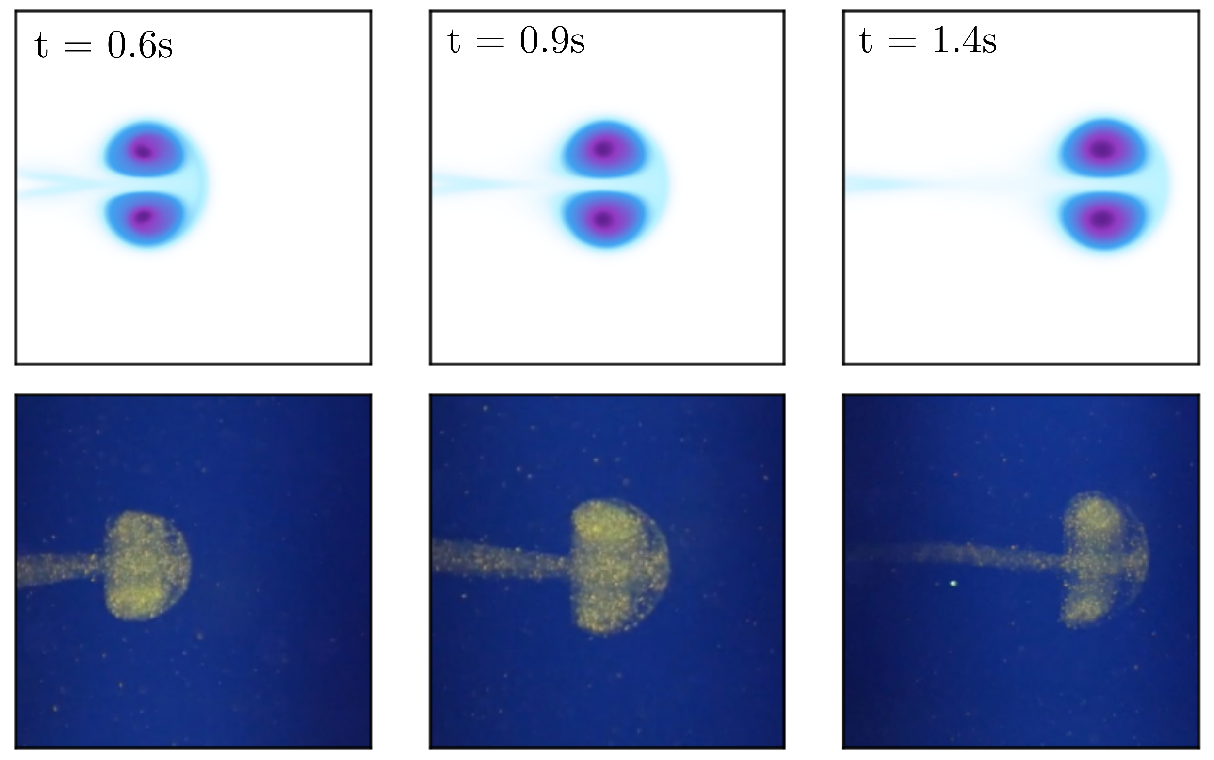
13]. We come to the same conclusions via conducted numerical simulations. In the following, the mentioned facts are discussed in detail. Additionally, Figure 3 illustrated the correspondence between simulation and experimental images of the vortex ring evolution.

3. Analytical Approximations

3.1. Velocity Field

First, let us consider the velocity vector field of a vortex ring moving in a given direction (downwards, following the experimental setup) at a fixed moment (similar to the vector field shown in Figure 2). The velocity field vectors rotate clockwise on the left part of the ring and counter-clockwise on its right part, concerning the direction of motion of the ring. In the center of the vortex ring, the two rotations are superimposed, and the vectors are directed downwards. As the horizontal distance from the ring center increases, the absolute values of the velocity vectors decrease, and this dependence is described by some function f ( r ) .
On a 2D cross-section of the 3D rotationally invariant velocity field, in the first approximation, the rotation on the left and right parts of a vortex ring can be described with two unit vectors of angular velocity w 1 and w 2 , which are directed toward the observer on the left part of the ring and away from the observer on the right one, respectively. The superposition of the two rotations can be written as:
v = ( w 1 × r 1 ) f ( r 1 ) + ( w 2 × r 2 ) f ( r 2 ) ,
where r 1 and r 2 are vectors from the centers of rotation to an observation point A . On the one hand, this superposition applies for near-lamellar flows with large Reynolds numbers, and on the other hand, it is the viscosity that is responsible for vortex formation, which allows us to introduce the decay function f. In addition to the angular velocity vectors and the decay function, a vortex ring model should include the distance between the rotation centers δ . The best ansatz for exact 3D simulations was found to be:
f ( r ) = a exp r c / b .
We have chosen this function as a result of a trial-and-error approach after considering various polynomial and exponential functions and their combinations. The coefficient b is measured in [ m ] c , and it can be interpreted as the “blurring” of vortex rings during propagation.
While this approximation seems to be adequate, it can be further improved to predict more specific properties of a vortex ring, e.g., its asymmetry along the direction of motion. For this reason, we will consider two pairs of rotation centers, where the two left centers have rotations in the same direction, as well as the two right ones:
v = i = 1 4 ( w i × r i ) f ( r i )
with the same function f given by Equation (3). In this model, suitable parameters of the velocity field stretch the ring, creating a little “tail”.
Figure 4 illustrates the application of Equations (3) and (4). Ring centers stretch the field in the direction of propagation of the vortex ring, which allows the approximation to accurately reproduce realistic shapes, and the relative error is less than 5 % compared to the rigorous simulation results. In Figure 4, the superposition of two identical analytical rings with a vertical offset between their cores 4 mm is shown. By the analytical ring, we mean a field that is given formulaically (4).

3.2. Temporal Evolution of a Vortex Ring

As a vortex ring propagates, the coefficients of the shape function f ( r ) become time-dependent. Using rigorous simulations, we approximated this dependence by minimizing the sum error of the two velocity projections at each time step. An important finding is that the coefficients demonstrate a monotonic time dependence after a specific moment of time t 0 , which will be shown further, together with explicit examples.
The temporal propagation of a vortex ring along its symmetry axis is well approximated by the logarithmic law, which was experimentally proved by Scase and Dalziel [31]:
z ( t ) = ln ( μ v 0 t + 1 ) μ ,
where v 0 is the initial velocity and μ is a positive constant. Writing the drag force in the form
F D = C D ρ v 2 2 S ,
the second Newton’s law yields the following explicit expression for the constant:
μ = C D S / 2 V .
Here, V is the characteristic volume of a vortex ring and S is its frontal area; thus, the ratio V / S indicates the ring thickness and is approximately constant. The coefficient V / S also plays an important role in the characteristic radius of the ring.

3.3. Particle Concentration

As mentioned above, our numerical simulations revealed that if a vortex ring propagates for a relatively long time, the spatial vorticity distribution ω becomes Gaussian, which agrees with the results of [26]. Additionally, while analyzing the simulation data, we discovered that the colloidal particles’ dilute concentration is distributed quite similar to ω , and therefore, we can assume the following approximation:
n = N · | curl ( v ) | .
with a time-dependent coefficient N ( t ) . Figure 5 and Figure 6 prove this assumption to be valid. Thus, in Figure 5, the vorticity modulus and the dilute concentration have the same spatial distribution, which can be accurately fit by a superposition of two Gaussian curves. The profile of | c u r l ( v ) | is not smooth because of the linear interpolation of the velocity field usage. To optimize the calculation time, it was decided to increase the calculation step. Despite this simplification, we can note that the type of dependence repeats the results of the Gaussian profile and the normalized particle concentration. In Figure 6, we can see that the relation between | curl ( v ) | and n is close to linear. For N ( t ) , we found a good approximation to be
N ( t ) = N 0 [ ( 1 h ) exp ( κ t ) + h ] 1 ,
where 0 < h < 1 . The time dependence given by this equation and its comparison with the ratio n / | curl ( v ) | extracted from numerical simulations is demonstrated in Figure 7, revealing a very good approximation accuracy.

3.4. Particle Loss Mechanism

Based on our research, we suggest that the main reason why particles trapped in the vortex ring are being lost is that there is an area in the back of the ring with a forward velocity less than the average velocity of the ring. Therefore, the particles suspended in this area are left behind the ring, forming a characteristic trail.
A sufficiently accurate approximation of this effect can be derived using the given vortex ring description, Equations (2) and (4), and the vortex evolution of Equations (8) and (9). Since we operate in a 2D space, the concentration is measured in [ 1 / m 2 ] . Then, the amount of particles at the moment t is:
N ( t ) = S | curl v | N ( t ) d S = S a b | exp ( x x 1 ) 2 + y 2 c / 2 b 2 b c ( x x 1 ) 2 + y 2 c / 2 + exp ( x + x 1 ) 2 + y 2 c / 2 b c ( x + x 1 ) 2 + y 2 c / 2 2 b | N ( t ) d S .
This integral can be efficiently evaluated numerically. In the following, we compare this formula, simulation results, and experimental data.

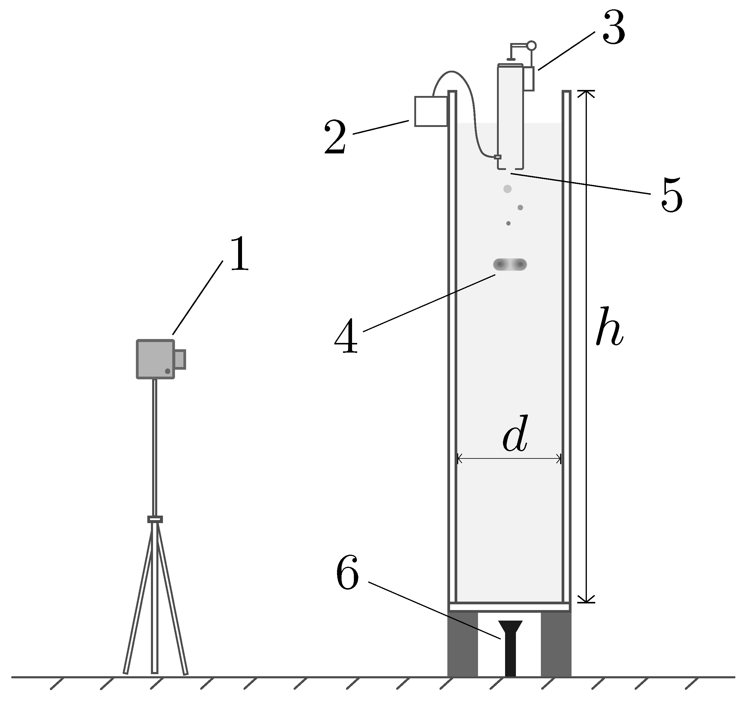
4. Experimental Setup and Measurements

The scheme of the experimental setup is shown in Figure 8. The main tank made of dense organic glass with a height of h = 0.3 m and width d = 0.11 m was filled with water. The rings themselves were generated with a plastic syringe with a diameter of 2 cm, a height of 8 cm, and an outlet with a diameter varied from 2 to 6 mm. The tank size was selected in such a way as to avoid the significant influence of wave reflection from the walls. Since the outlet size is in millimeters and the tank diameter is 10 centimeters, the influence of the walls on propagating rings can be neglected based on the results of velocity field modeling for a large vortex ring (see Figure 4). All the equipment was placed on top of the tank. A movable piston controlled by a servo drive and microcontroller was placed inside the syringe. Color dyes and colloidal particles (titanium dioxide beads about 1 μ m in size) were injected through a hole about 2 mm in diameter in the lower part of the syringe. This setup allowed us to create a long series of vortex rings and precisely set such parameters as the initial speed and radius. To measure the rings’ coordinates and radii, and the concentration of the colloidal particles, we used cameras with the following parameters: f = 26 mm, aperture f / 1.6 , frame rate between 25 and 60, and resolution 3840 × 2160 . Since the bottom of the pipe was also made of transparent plexiglass, the design allowed us to take images of the vortex rings both from the side and the bottom of the tank. An LED panel was installed behind the setup, giving even white light, which helped to recognize the boundaries of toroidal vortices more accurately. For detection, we used either particles glowing in the ultraviolet or the rhodamine dye that glows yellow in the violet spectrum. We placed an ultraviolet LED flashlight under the transparent bottom of the tank to illuminate the liquid. We studied the vortex ring propagation under various conditions, including changing the initial temperature, which was set in the range of 20–50 °C. The Reynolds numbers in our installation varied in the range R e ( 3000 ; 13,000).
It is worth saying that since the observation was conducted through glass, it is necessary to take into account the possible distortions of the resulting image. Therefore, we minimized these effects by using a water tank with smooth walls, recording video from a long distance to reduce the influence of perspective, and spot-highlighting the ring from the bottom of the tank to eliminate glare on the glass. Also, due to the relatively small size of the objects compared to the size of the vessel and the distance to the camera, the resulting distortions are insignificant.
We performed two sets of experiments. In the first set, we created single vortex rings and investigated their behavior in a viscous fluid to test the applicability of the theoretical model for the velocity field. Using a pumping device, we supplied a soluble dye directly in front of the outlet, which allowed us to directly colorize the rings. In the second set, the same rings were carrying the colloidal particles, and we studied the dependence of the number of particles delivered by rings on time and coordinate. We used titanium dioxide micro-beads 1 μ m in size. The chosen experimental conditions allowed us to neglect the influence of the particles on the vortex flows’ behavior.
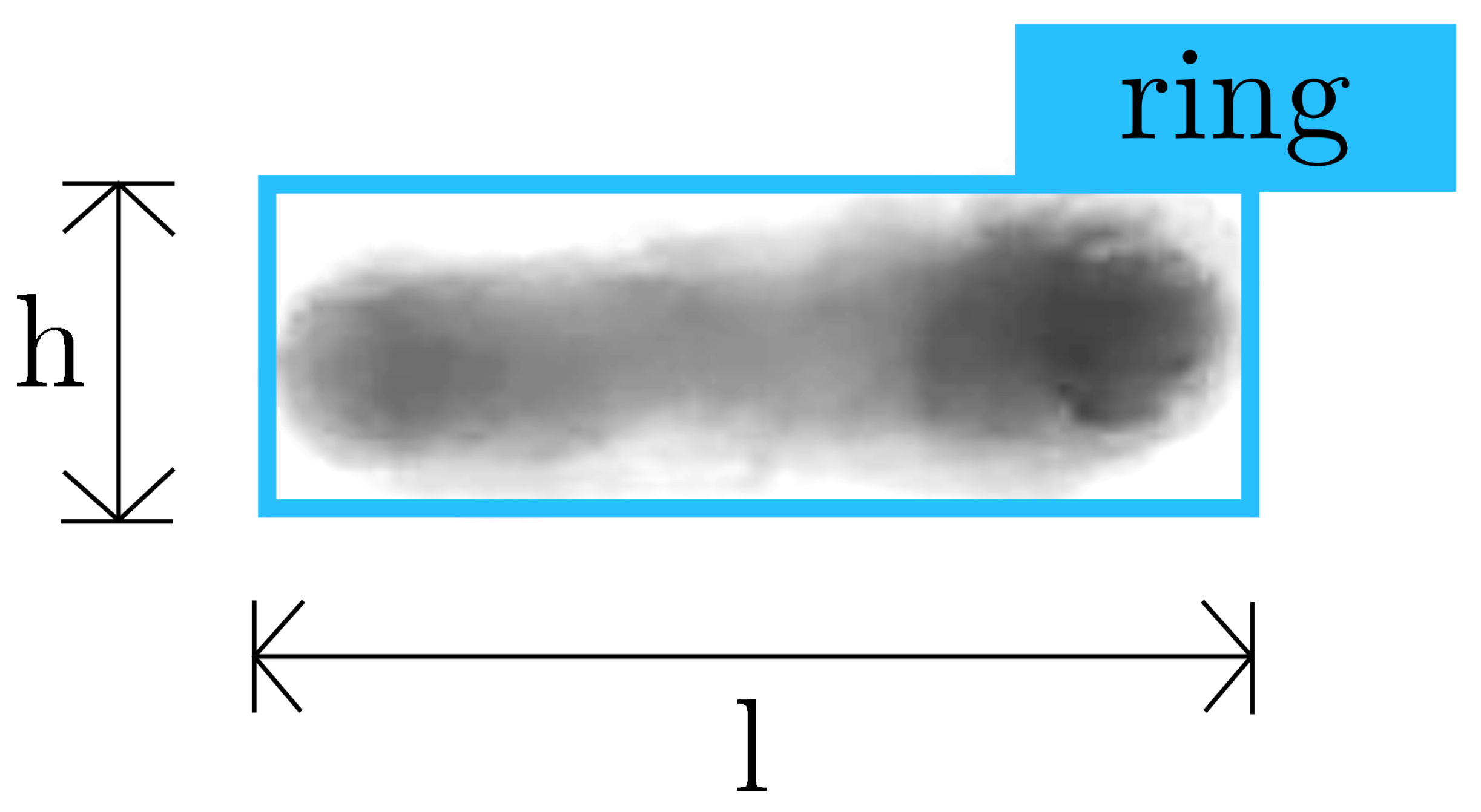
With experimental measurements, we obtained the following key parameters: the position and radius of the vortex rings, and the time-dependent number of particles trapped in the rings. To determine the positions and radii of the rings, a neural network was used on the slide-shot video. The neural network used was YOLOv5s by Ultralytics—the one-stage detector convolutional neural network. It helped to quickly process the experimental data. YOLOv5s was chosen because it is simple to configure a ready solution, has a generally pre-trained version, and it is fast and accurate enough in the current application. It was additionally trained on a manually processed data set consisting of photographs of the rings. The obtained results were verified with the “Tracker Physics” software (ver. 6.1.3) [32]. “Tracker” provides semi-automatic object tracking with the ability of manual correction both during the position tracking and calibration with a reference scale presented in the video. To model a ring as an ideal toroid, the images were fit into rectangles with sides h and , as shown in Figure 9, thus giving the small and large torus radii r = h / 2 , R = [ 2 h ] / 2 , respectively.
Particles in a colloid are too small to be counted directly. Therefore, we estimated their density indirectly, using the amount of backscattered radiation. Assuming the density is low enough for the multiple scattering effect to be neglected, the dependence of the backscattered intensity I b coming to the camera from the colloidal particles with a concentration n and optical thickness l should be exponential:
I b = I 0 1 exp ( C n l ) .
The above assumptions leading to this functional dependence were verified by measuring the intensity as a function of n.
The obtained images of propagating vortex rings were pixelated and converted to grayscale so that the relation between the pixel brightness B i and the number of particles N i in the pixel area S i can be written in a similar form:
B i = B 0 1 exp ( C B N i / S i ) .
where B 0 and C B are constants, and the index i enumerates the pixels. The latter equation yields the formula for the determination of the relative particle density
N i / N 0 ln 1 B i / B 0 ,
provided that S i is the same for all pixels. By summation over all the pixels of a vortex, we can estimate the total amount of particles within a vortex ring.

5. Results and Discussions

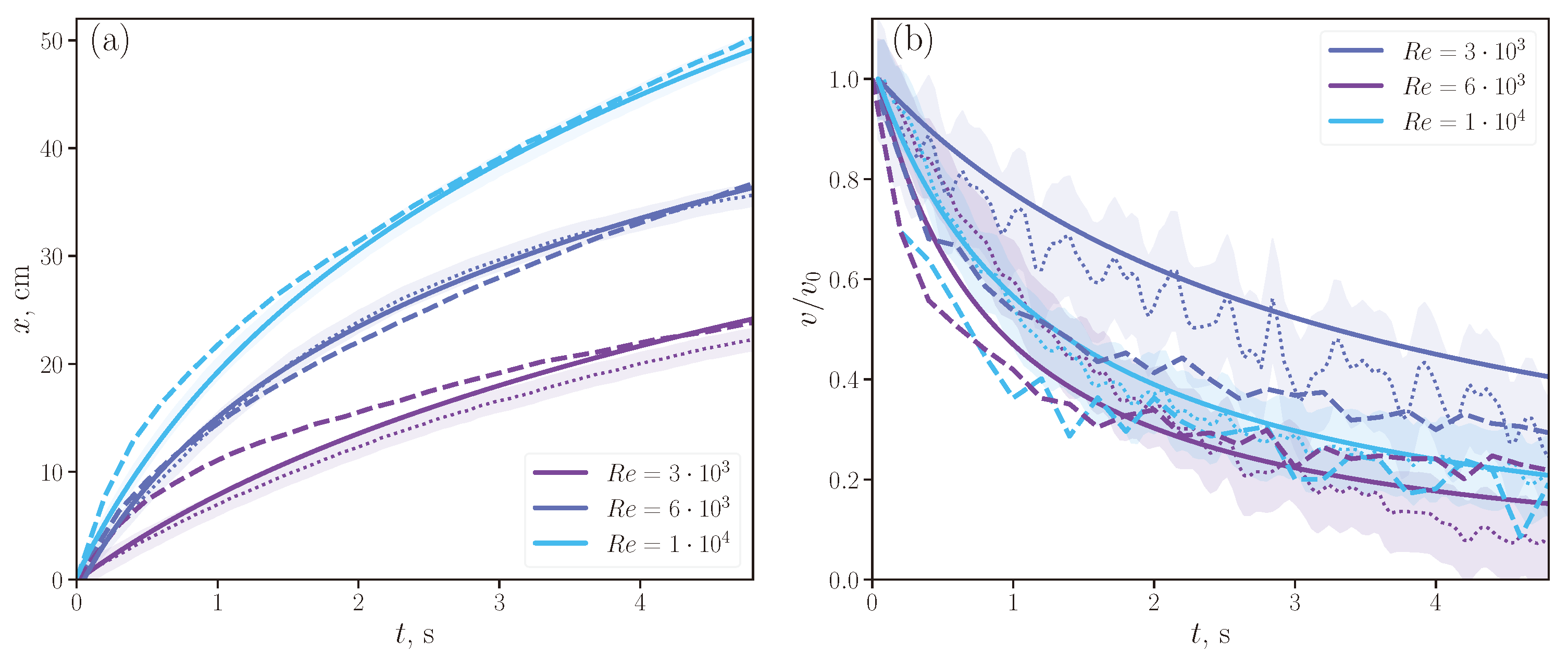
To describe the general motion of the vortex ring, we considered rings without particles both in experiments and in numerical modeling. We wanted to obtain general ideas about the nature of the movement, which is displayed in Figure 10. We compare the time-dependent coordinates and velocities obtained with the simulation, the equations, and experimental measurements for the vortex rings free of particles. The coordinates are calculated with Equations (5) and (7), and the velocity model is obtained by the differentiation of Equation (5), which results in the following time dependence:
v = C D S 2 V t + 1 U 0 1 .
As was already stated, the ratio V / S in (7) is approximately constant, so the vortex velocity in the propagation direction can be estimated to be inversely proportional to the travel time. The best fit for the drag constant was found to be C D 0.03 . The theory and experiment are in good agreement, and the obtained data suggest that the proposed simple model is applicable in a wide range of initial Reynolds numbers, which characterize the vortex motion by formula R e = 2 u 0 / ν .
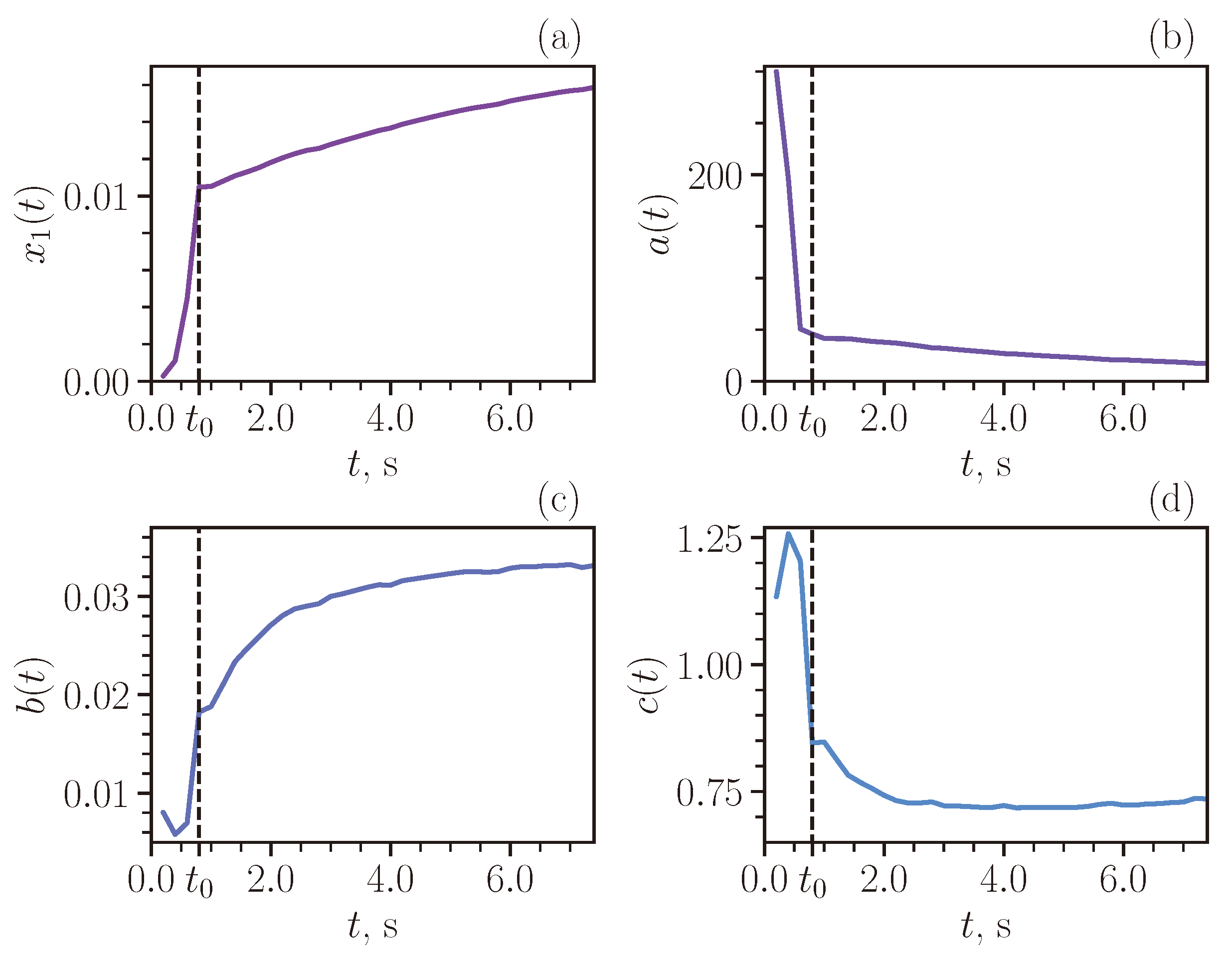
Coefficients describing the ring shape in Equation (3) were extracted from the experimental data, and their time dependence is shown in Figure 11. This result demonstrates that two propagation modes exist. First, at the initial moment, for a time less than a second, the vortex ring may dramatically change its geometry. This process can be interpreted as a formation process of a vortex ring. Second, after an abrupt transition, the geometry begins to vary slowly, with the parameters a, b, and c changing almost monotonically.
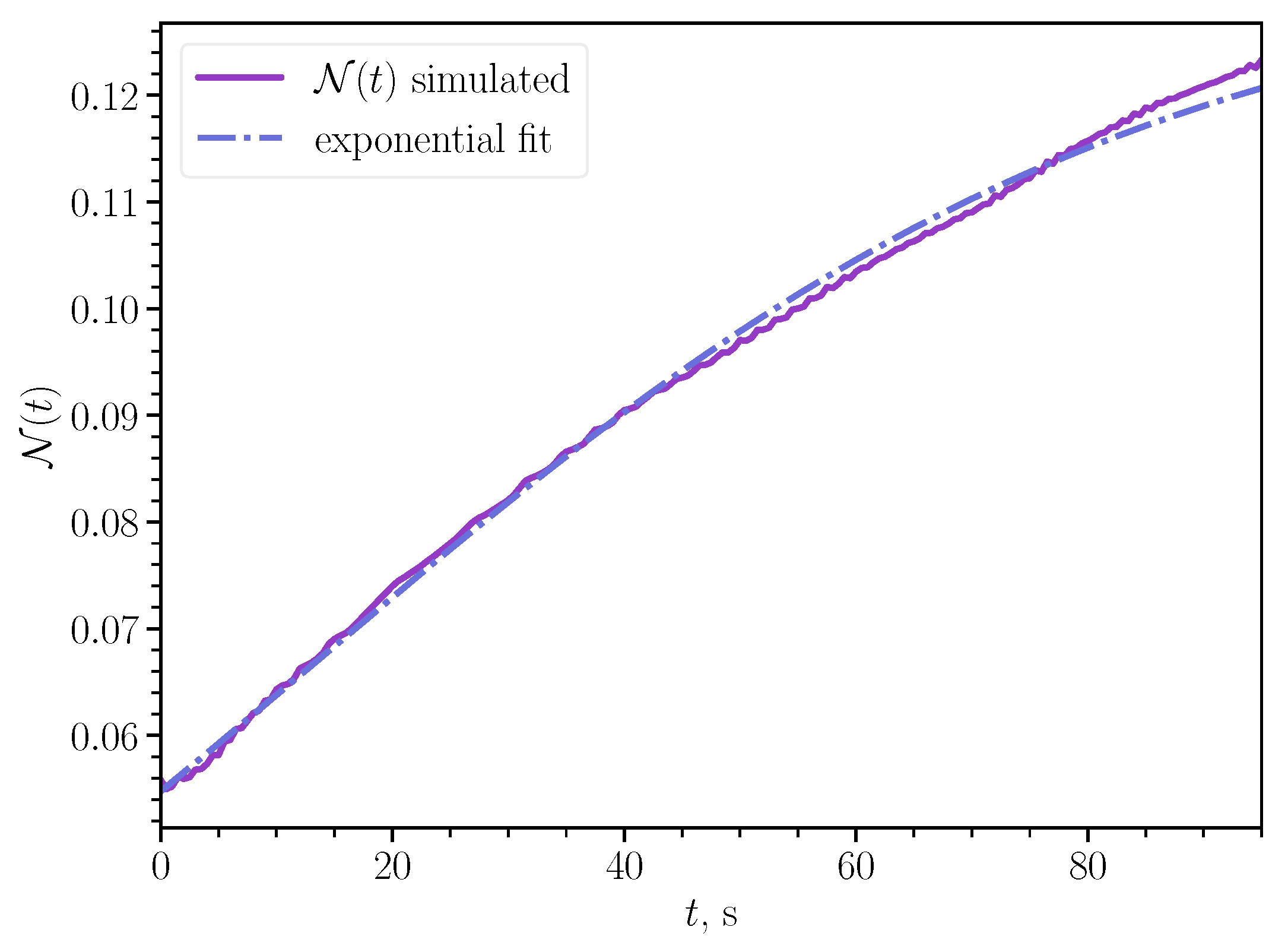
The particle loss process for vortex rings carrying particles is illustrated in Figure 12. The plotted experimental error comes from the standard deviation obtained in a series of experiments with the same initial conditions. The simulation error was estimated to be about 5 % , and it stems from the Comsol model assumption and the uncertainties in the determination of the ring boundaries. The experiments and simulations reveal that the particle loss mechanism consists of lagging of particles in the rear part of the vortex ring due to lower velocities in this spatial domain.

6. Conclusions

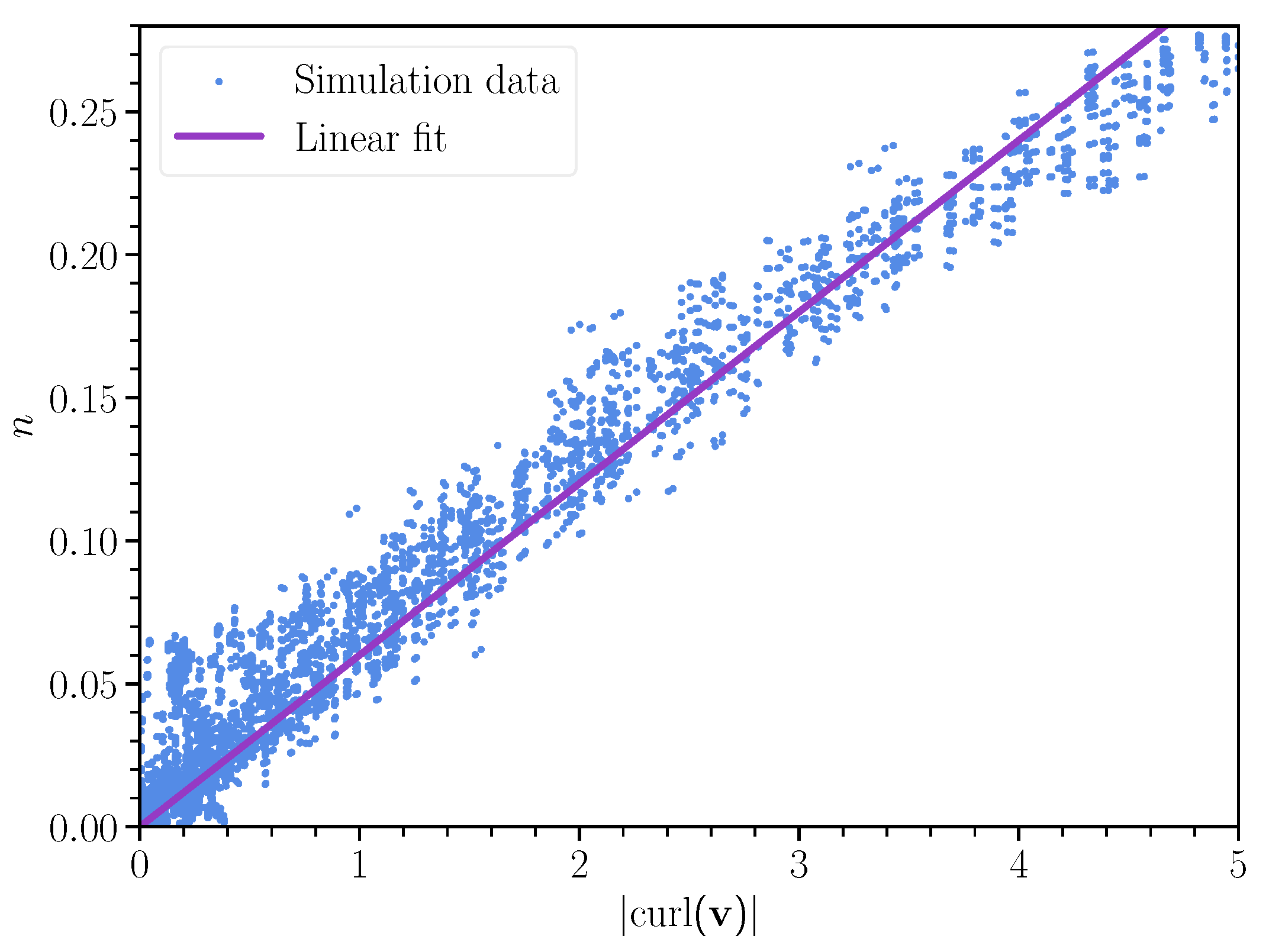
To summarize, in this work, we have proposed a simple analytical approximation for the vortex ring velocity field and analyzed the time evolution of the parameters of this approximation. The consistency of numerical simulations in COMSOL Multiphysics, calculations and experimental results proved the validity of the chosen 2D model. Our results reveal a direct correspondence between the vorticity and particle density for rings carrying colloids, which allowed us to find a simple approximation for a time-dependent dilute concentration of the particles trapped in a vortex ring.
We believe that our findings have potential applications in setups for biochemical applications, such as the spatial delivery of substances in liquid solutions. As the dilute concentration is proportional to the vorticity, the spatial delivery of particles could create a preassigned density or viscosity gradient in the solution.
The obtained results can form the basis for further studies of toroidal vortices as a method of transporting particles in viscous liquids. In the future, we plan to study the transport of particles in vortex rings with Reynolds numbers in the range from 10 to 100,000. In addition, of practical interest is the study of the efficiency of delivery of particles whose dimensions are comparable to the linear dimensions of the vortex ring.

Author Contributions

Conceptualization, D.S., I.Z., V.G. and A.K.; formal analysis, D.S., R.P., A.K. and I.Z.; methodology, Z.S. and A.K.; software: F.K.; investigation, V.G., D.S., I.Z., F.K. and R.P.; visualization, I.Z., F.K., R.P., V.G. and D.S.; writing—original draft preparation, V.G., D.S. and R.P.; supervision, Z.S., M.K., Y.M. and A.K.; validation, Z.S.; resources: M.K. and Y.M.; funding acquisition, Y.M.; project administration, A.K.; writing—review and editing, A.K. All authors have read and agreed to the published version of the manuscript.

Funding

This research was supported by Priority 2030 Federal Academic Leadership Program.

Data Availability Statement

The data presented in this study are available on request from the corresponding author.

Acknowledgments

It is a pleasure to thank Alexey A. Shcherbakov for fruitful discussions.

Conflicts of Interest

The authors declare no conflict of interest.

References

  1. Akhmetov, D.G. Vortex Rings; Springer: Berlin/Heidelberg, Germany, 2009. [Google Scholar]
  2. Meleshko, V.V.; Gourjii, A.A.; Krasnopolskaya, T.S. Vortex rings: History and state of the art. J. Math. Sci. 2012, 187, 772–808. [Google Scholar] [CrossRef]
  3. Fraenkel, L.E. Examples of steady vortex rings of small cross-section in an ideal fluid. J. Fluid Mech. 1972, 51, 119–135. [Google Scholar] [CrossRef]
  4. Auerbach, D. Stirring properties of vortex rings. Phys. Fluids A 1991, 3, 1351–1355. [Google Scholar] [CrossRef]
  5. Tarasov, V.F.; Yakushev, V.I. Transport in a turbulent vortex ring. J. Appl. Mech. Tech. Phys. 1975, 15, 106–110. [Google Scholar] [CrossRef]
  6. Nikulin, V.V. Mass Exchange between the Atmosphere of Turbulent Vortex Ring and the Surrounding Medium. Fluid Dyn. 2021, 56, 473–480. [Google Scholar] [CrossRef]
  7. Rakhsha, M.; Kees, C.E.; Negrut, D. Lagrangian vs. Eulerian: An Analysis of Two Solution Methods for Free-Surface Flows and Fluid Solid Interaction Problems. Fluids 2021, 6, 460. [Google Scholar] [CrossRef]
  8. Moraes, P.G.d.; Oliveira, M.A.d.; Bimbato, A.M.; Pereira, L.A.A. A Lagrangian Description of Buoyancy Effects on Aircraft Wake Vortices from Wing Tips near a Heated Ground Plane. Energies 2022, 15, 6995. [Google Scholar] [CrossRef]
  9. Griffiths, D.A.; Ananthan, S.; Leishman, J.G. Predictions of Rotor Performance in Ground Effect Using a Free-Vortex Wake Model. J. Am. Helicopter Soc. 2005, 50, 302–314. [Google Scholar] [CrossRef]
  10. Akhmetov, D.G.; Lugovtsov, B.A.; Maletin, V.A. Vortex Powder Method for Extinguishing a Fire on Spouting Gas—Oil Wells. In Prevention of Hazardous Fires and Explosions; Springer: Dordrecht, The Netherlands, 1999; pp. 319–328. [Google Scholar] [CrossRef]
  11. An, D.; Warning, A.; Yancey, K.G.; Chang, C.T.; Kern, V.R.; Datta, A.K.; Steen, P.H.; Luo, D.; Ma, M. Mass production of shaped particles through vortex ring freezing. Nat. Commun. 2016, 7, 12401. [Google Scholar] [CrossRef]
  12. Akagi, F.; Haraga, I.; ichi Inage, S.; Akiyoshi, K. Effect of sneezing on the flow around a face shield. Phys. Fluids 2020, 32, 127105. [Google Scholar] [CrossRef]
  13. Sullivan, I.S.; Niemela, J.J.; Hershberger, R.E.; Bolster, D.; Donnelly, R.J. Dynamics of thin vortex rings. J. Fluid Mech. 2008, 609, 319–347. [Google Scholar] [CrossRef]
  14. Kida, S.; Takaoka, M.; Hussain, F. Collision of two vortex rings. J. Fluid Mech. 1991, 230, 583–646. [Google Scholar] [CrossRef]
  15. Cheng, M.; Lou, J.; Lim, T.T. Collision and reconnection of viscous elliptic vortex rings. Phys. Fluids 2019, 31, 067107. [Google Scholar] [CrossRef]
  16. Mouallem, J.; Daryan, H.; Wawryk, J.; Pan, Z.x.f.x.a.; Hickey, J.P. Targeted particle delivery via vortex ring reconnection. Phys. Fluids 2021, 33, 103305. [Google Scholar] [CrossRef]
  17. Domon, K.; Ishihara, O.; Watanabe, S. Mass Transport by a Vortex Ring. J. Phys. Soc. Jpn. 2000, 69, 120–123. [Google Scholar] [CrossRef]
  18. Uchiyama, T.; Yano, C.; Degawa, T. Generation and Transport of Solid Particle Clusters Using a Vortex Ring Launched into Water. Int. J. Chem. Eng. Appl. 2017, 8, 253–260. [Google Scholar] [CrossRef]
  19. James, S.; Madnia, C.K. Direct numerical simulation of a laminar vortex ring. Phys. Fluids 1996, 8, 2400–2414. [Google Scholar] [CrossRef]
  20. Danaila, I.; Hélie, J. Numerical simulation of the postformation evolution of a laminar vortex ring. Phys. Fluids 2008, 20, 073602. [Google Scholar] [CrossRef]
  21. Weigand, A.; Gharib, M. On the decay of a turbulent vortex ring. Phys. Fluids 1994, 6, 3806–3808. [Google Scholar] [CrossRef]
  22. Rosenfeld, M.; Rambod, E.; Gharib, M. Circulation and formation number of laminar vortex rings. J. Fluid Mech. 1998, 376, 297–318. [Google Scholar] [CrossRef]
  23. Sullivan, J.P.; Widnall, S.E.; Ezekiel, S. Study of Vortex Rings Using a Laser Doppler Velocimeter. AIAA J. 2012, 10, 11. [Google Scholar] [CrossRef]
  24. Dziedzic, M.; Leutheusser, H.J. An experimental study of viscous vortex rings. Exp. Fluids 1996, 21, 315–324. [Google Scholar] [CrossRef]
  25. Fung, J.C.H. Residence time of inertial particles in a vortex. J. Geophys. Res. Ocean. 2000, 105, 14261–14272. [Google Scholar] [CrossRef]
  26. Saffman, P.G. The Velocity of Viscous Vortex Rings. Stud. Appl. Math. 1970, 49, 371–380. [Google Scholar] [CrossRef]
  27. Tinaikar, A.; Advaith, S.; Basu, S. Understanding evolution of vortex rings in viscous fluids. J. Fluid Mech. 2018, 836, 873–909. [Google Scholar] [CrossRef]
  28. Guide, C.M.U. Mixer Module User’s Guide; COMSOL: Stockholm, Sweden, 2021. [Google Scholar]
  29. Visuri, O.; Wierink, G.A.; Alopaeus, V. Investigation of drag models in CFD modeling and comparison to experiments of liquid–solid fluidized systems. Int. J. Miner. Process. 2012, 104–105, 58–70. [Google Scholar] [CrossRef]
  30. Silva, R.; Cotas, C.; Garcia, F.A.P.; Faia, P.M.; Rasteiro, M.G. Particle Distribution Studies in Highly Concentrated Solid-liquid Flows in Pipe Using the Mixture Model. Procedia Eng. 2015, 102, 1016–1025. [Google Scholar] [CrossRef]
  31. Scase, M.M.; Dalziel, S.B. An experimental study of the bulk properties of vortex rings translating through a stratified fluid. Eur. J. Mech. B Fluids 2006, 25, 302–320. [Google Scholar] [CrossRef]
  32. Tracker Video Analysis and Modeling Tool for Physics Education. 2023. Available online: https://physlets.org/tracker/ (accessed on 23 May 2023).
Figure 1. Photo image of a vortex ring colored with a dye.
Fluids 08 00315 g001
Figure 2. Example of the initial velocity field used to form the rings in simulations. The white rectangle indicates the area where the colloidal particles were initially placed. The color bar indicates the absolute value of the velocity at each point.
Fluids 08 00315 g002
Figure 3. Time evolution of a vortex ring: (lower panel) experimental pictures, and (upper panel) simulation.
Fluids 08 00315 g003
Figure 4. Vortex velocity field simulated at a fixed time moment with Equations (3) and (4).
Fluids 08 00315 g004
Figure 5. Modulus of the vorticity | curl ( v ) | , dilute concentration n, and a fit comprising two Gaussian curves in the vortex cross-section orthogonal to the propagation direction.
Fluids 08 00315 g005
Figure 6. Correlation between the vorticity and dilute concentration at a fixed time moment and the best linear fit. Different points in the plot correspond to different spatial points.
Fluids 08 00315 g006
Figure 7. Coefficient N ( t ) calculated with Equation (9) and extracted from Comsol simulations as a ratio n / | curl ( v ) | .
Fluids 08 00315 g007
Figure 8. Experimental setup: (1) video camera; (2) source of a dye or colloidal particles; (3) automatic drive for control of vortex ring formation; (4) propagating vortex ring; (5) outlet of the injection tube; (6) UV flashlight.
Fluids 08 00315 g008
Figure 9. Vortex ring with characteristic dimensions.
Fluids 08 00315 g009
Figure 10. Dependence of the vertical coordinate of a vortex ring (a) and its velocity (b) on time. Experimental data are shown with dotted lines, with errors indicated by shaded areas; theoretical data are shown with solid lines; numerical simulation results are shown with dashed lines. Different colors correspond to different initial Reynolds numbers.
Fluids 08 00315 g010
Figure 11. Time-dependent coefficients of the theoretical function describing the vortex ring shape. Panel (a) shows the distance x 1 from the center of the ring to one of its cores, so x 1 makes sense of the main radius of the ring R, it appears in (10). Panels (bd) show the coefficients of f u = a exp ( r c / b ) , a, b and c, respectively. Also, the moment of time t 0 is marked in all the figures, it makes sense of the end of the transition period of the ring. Since in modeling the ring is formed according to the primary approximate formula, at the beginning of its evolution it naturally changes shape to its characteristic appearance. Therefore, for approximately the first second, the shape of the ring is extremely non-standard, therefore, the coefficients change very sharply at the beginning, but after the time t 0 , they acquire a monotone dependence.
Fluids 08 00315 g011
Figure 12. Time dependence of the relative number of particles N r e l ( t ) = N / N 0 carried by vortex rings. The experimental and modeling results are shown with light blue and violet colors, respectively. Theoretical calculation results are shown with a dashed line. The shaded areas’ width illustrates the error.
Fluids 08 00315 g012
Disclaimer/Publisher’s Note: The statements, opinions and data contained in all publications are solely those of the individual author(s) and contributor(s) and not of MDPI and/or the editor(s). MDPI and/or the editor(s) disclaim responsibility for any injury to people or property resulting from any ideas, methods, instructions or products referred to in the content.

